Influence of the Trailing Edge Shape of Impeller Blades on Centrifugal Pumps with Unsteady Characteristics

Abstract

The flow field structure and pressure pulsation characteristics in two series of trailing edges of a centrifugal pump are investigated using the SST k-w turbulence model. Series 1 involves varying the impeller exit angle, and Series 2 involves varying the impeller exit shape. The entropy generation rate analysis method is used to evaluate the numerical simulation results. Vortex cores within the flow field are identified by applying the Ω criterion. The influence of different trailing edge configurations on the energy loss characteristics of the pumps is explored. The dynamic mode decomposition (DMD) method is used to analyze pressure pulsations at the volute considering unsteady flows in centrifugal pumps with different trailing edge shapes. The findings suggest that different trailing edge shapes can be used to adjust the energy loss proportions in various components of the pump. In Series 1, the efficiency remains nearly constant with changes in the outlet angle on both sides of the trailing edge. In Series 2, the efficiency is enhanced by 1.18% with the elliptical edge shape on both sides (EBS) compared to the original trailing edge (OTE) shape. In Series 1 and Series 2, greater entropy generation rates are accompanied by greater pressure pulsations at the pump outlet. The DMD results demonstrate a noticeable impact of the different trailing edges on the pressure distribution of various modes within the volute. Moreover, the impeller outlet pressure inhomogeneity coefficient changes under different modes. This study holds great significance for selecting the appropriate trailing edges for centrifugal pumps.

1. Introduction

Centrifugal pumps are extensively used as power machinery in pipelines and flow systems. The key sources of fluid excitation within centrifugal pumps include impeller–volute interactions as well as unstable flow structures, such as shedding vortices behind the trailing edges [1]. The shape of the impeller’s trailing edge is closely linked to rotor-stator interaction, wake flows, and jets. Therefore, it is crucial to analyze different trailing edge profiles to gain a better understanding of their impact on the flow field and pressure pulsation characteristics in the pump.

The mainstream approach to blade edge modifications involves employing similar offset and cutting operations from the shroud to the hub [2,3,4,5,6,7]. Some scholars have also modified the trailing edge unilaterally. Zhang et al. [2] conducted cutting operations on the pressure side of the blade trailing edge, effectively improving the uniformity of the blade exit. Similarly, Huang et al. [3] implemented unilateral pressure-side cutting to reduce the exit angle of the impeller’s pressure surface, thereby adjusting the velocity component at the impeller exit and influencing the pressure pulsations within the pump. Some researchers have attempted to simultaneously modify both the pressure and suction sides. For example, Cui et al. [4] used large eddy simulations and fluid–structure coupling methods to apply identical cutting angles to both sides of the trailing edge; this resulted in a reduced average vortex intensity and a smaller wake area at the rated flow. Other studies have implemented curved edge modifications. Gao et al. [5] modified the pressure and suction sides of the trailing edge of a low-specific speed centrifugal pump into an elliptical shape, effectively reducing the vortex strength at the blade trailing edge and weakening the interaction between the rotor and stator. Wu et al. [6] analyzed the influence of seven different trailing edge radii on the local Eulerian head distribution and concluded that the local Eulerian head is closely linked to the pump efficiency. Zhang et al. [7] employed a genetic algorithm combined with fuzzy logic as an optimization strategy for minimizing pressure pulsation intensity, focusing on optimizing the shape of the blade trailing edge. Some researchers have also analyzed the non-uniform distribution of the flow field by altering the blade trailing edge from the hub to the shroud. Li et al. [8] applied sine nodules to the suction side of the blade trailing edge, effectively altering the vortex structure and intensity in the trailing edge region. By inserting a sine shape into the trailing edge and introducing the entropy production rate analysis method, Lin et al. [9] demonstrated that this structure reduced the total energy consumption. Wang et al. [10] analyzed the inclination degree of the blade trailing edge of a water pump, revealing that forward-leaning blades could suppress jet wake structures to some extent due to their local backflow effect.

With respect to the energy analysis of pumps, Denton et al. [11] were the first to conduct an extensive analysis of the entropy mechanism through mathematical derivations, identifying the fundamental origins of the loss of efficiency and establishing a proportional relationship between entropy generation and the cube of the relative surface velocity. In a related study, Sun et al. [12] implemented blade modifications using non-uniform rational B-splines, referencing two-dimensional blade section aerodynamic coefficients to explore an entropy-based approach for characterizing the performance of fluid machinery and enhancing efficiency. Wang et al. [13] further investigated the influence of increased compressor inlet angle on the dynamic losses of vortices, using entropy analysis to establish the relationship between turbulent dissipation effects and Reynolds shear stress. Similarly, Huang et al. [14] examined the entropy distribution and pressure pulsation within centrifugal pumps at different flow rates, considering turbulent dissipation rates and wall friction dissipation rates. Meanwhile, El-Gendi et al. [15] used delayed detached eddy simulations to investigate the relationship between energy losses and the transformation of turbine machinery from a circular to an elliptical trailing edge with varying aspect ratios. Hoseinzade et al. [16] optimized the local entropy integral and other objectives by altering the trailing edge angle of steam turbine blades, studying the impact of this angle on thermodynamic losses. They also examined the influence of the trailing edge thickness on the energy characteristics, such as blade profile losses and aerodynamic losses in the compressor [17]. Notably, several scholars have contributed to the analysis of blade profile optimization in pumps [18,19,20,21]. Regarding entropy generation with unsteady flow properties, it is also used in many other fields, such as non-newtonian second-grade nanoliquids [22] and the nonlinear dissipative flow of Sisko fluid [23].

In addition, there has been a growing interest towards analyzing the characteristic frequencies of pressure pulsations in the unsteady flow field of centrifugal pumps. Due to the typical frequency characteristics of the pressure pulsations of centrifugal pumps, the dynamic mode decomposition (DMD) method offers advantages in extracting the corresponding spatio-temporal turbulence structure at these frequencies. The DMD method was first proposed by Schmid [24,25], and with the development of experimental technology and numerical calculations, it has been widely employed in the analysis of various flow phenomena [26,27,28,29,30]. For example, the DMD method has been used to analyze the internal flow structures of rotating machinery [31,32,33,34,35,36]. DMD primarily focuses on analyzing the changes in a variable field at specific frequencies, with a significant impact on the flow field resulting from changes in the trailing edge. However, only a few studies have investigated the unsteady flow after a trailing edge change by examining field changes. Therefore, the DMD method is used in this study to analyze changes in the flow field following a trailing edge change.

This study uses CFD tools to investigate the impact of different impeller trailing edges on centrifugal pumps. Trailing edge modifications are divided into two categories: Series 1 involves changes in the outlet angle and Series 2 involves changes in the trailing edge shape. The entropy analysis method is used to quantitatively study the energy loss of the centrifugal pump, and the DMD method is used to analyze the modal energy proportions of different trailing edges. This research holds great significance in guiding the selection of trailing edges for centrifugal pumps.

2. Numerical Simulation Procedures

2.1. Pump Parameters

A Cartesian coordinate system was established in space, as illustrated in Figure 1a. The centrifugal pump consisted of an impeller with six blades and a volute. The detailed parameters are outlined in

Table 1. Main parameters of the centrifugal pump.

Item	Value
Rotational speed, $\omega$ (rad/s)	100π
Rotational frequency, fn (Hz)	50
Pump design head, $H$ (m)	66.5
Design flow rate, $Q$ (m3/h)	110
Number of impeller blades, Z	6
Type number, K	0.4257
Diameter of inlet, Dj (mm)	101
Diameter of outlet, D2 (mm)	238.7
Outlet width of the impeller, b2 (mm)	16.516
Cap nut diameter, Dh (mm)	53

. The type number is denoted as K ($K=\omega Q^{1/2}/60{\left(\mathrm{g}H\right)}^{3/4}$), while $g$ represents the acceleration of local gravity. As shown in Figure 1b, to ensure a stable and uniform flow as the liquid enters the impeller, an extension was made to both the impeller inlet section and the volute outlet section. The coordinate origin was located at the center of the impeller, with the right-hand rule determining the positive direction of the Z-axis as the rotational direction.

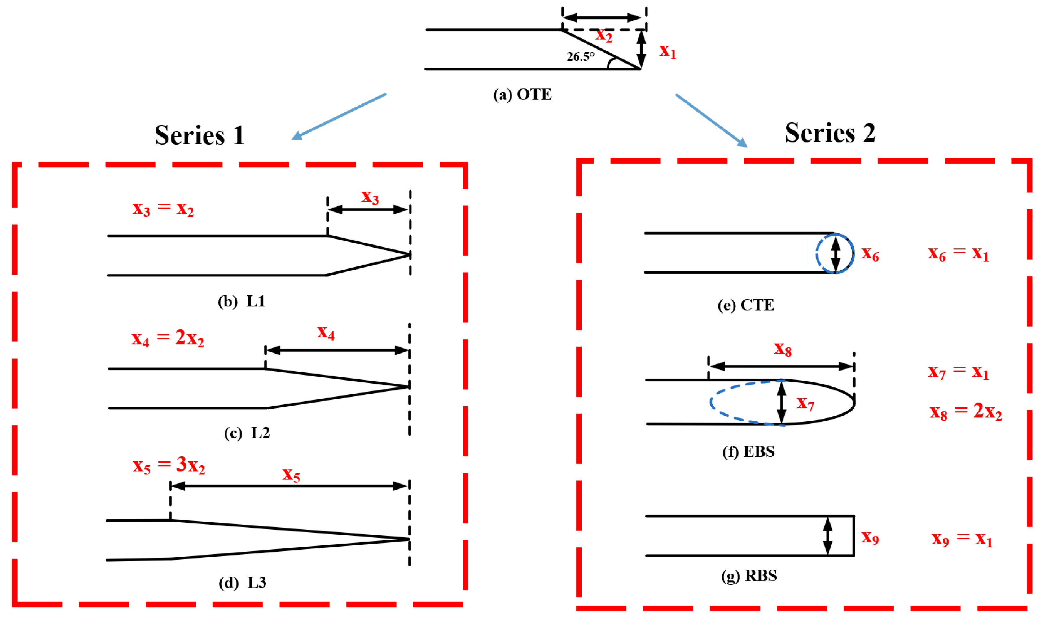
2.2. Blade Trailing Edge Profiles

In order to study the influence of the blade trailing edge profile on the internal flow characteristics and the pressure pulsation of the centrifugal pump, two series of trailing edge shapes were designed. Series 1 included the (a) original trailing edge (OTE) and trailing edges with different exit angles on both sides, i.e., (b) L1, (c) L2, and (d) L3. Series 2 included trailing edges with different shapes on both sides, i.e., (e) a circular trailing edge (CTE), (f) an elliptical edge on both sides (EBS), and (g) a rectangular edge on both sides (RBS). Figure 2 illustrates the length relationship of these designs. In Figure 2b–d, the suction surface and the pressure surface are symmetrical at the trailing edge, while the blade exit angle varies, and the details are shown in

Table 2. Length relationship of the different trailing edge shapes.

Different Trailing Edge Shapes	Item	Relationship or Value
OTE	x1	4.26 mm
OTE	Exit angle (α)	26.5°
OTE	x2	x2 = x1∙tanα
L1	x3	x3 = x1
L2	x4	x4 = 2x1
L3	x5	x5 = 3x1
CTE	Radius (x6)	x6 = x1
EBS	Minor axis (x7)	x7 = x1
EBS	Major axis (x8)	x8 = 2x1
RBS	x9	x9 = x1

.

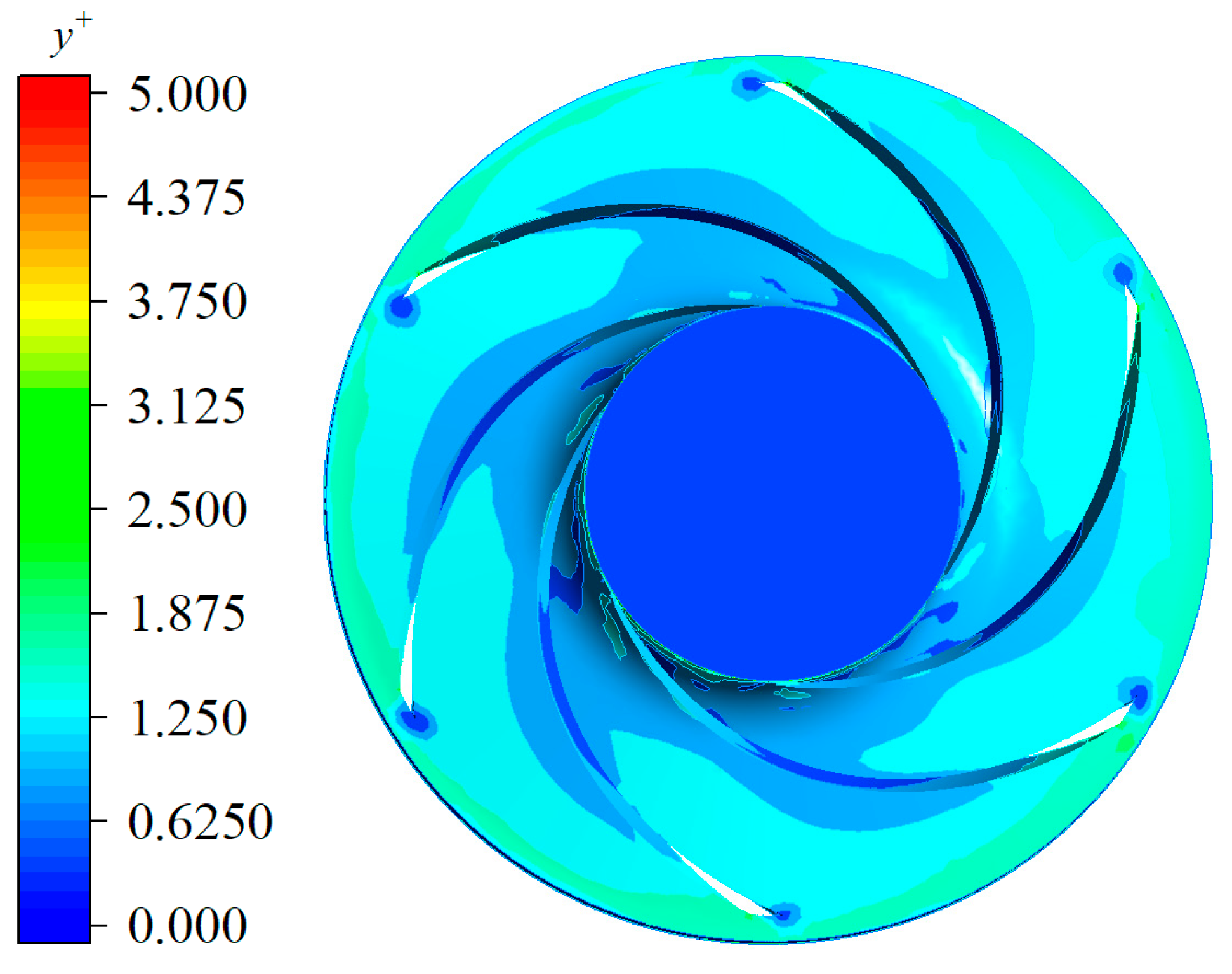
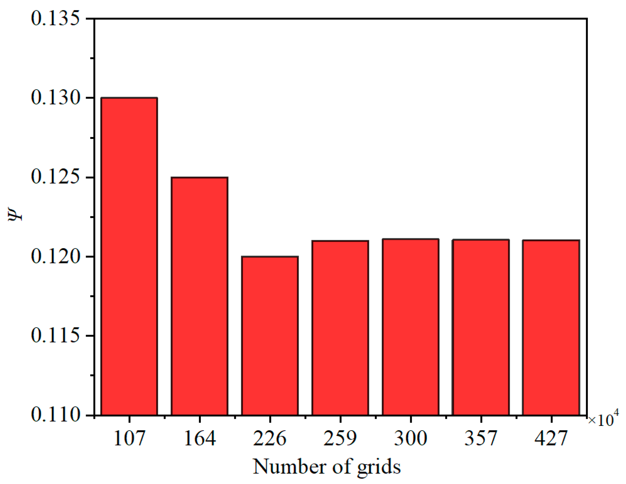
2.3. Numerical Method

The commercial computational fluid dynamics (CFD) software ANSYS CFX 17.0 was utilized to analyze the continuity and momentum equations for the internal flow of the pump. The turbulence was simulated using the SST k-w model [37,38,39,40]. In terms of the boundary conditions, a total pressure of 2 kPa was specified at the inlet, a mass flow rate condition of 30.5 kg/m³ was set at the outlet, and no-slip conditions were applied to the other wall surfaces. Due to the rotation of the impeller, two distinct computational domains were formed within the pump: the rotating impeller domain and the stationary domain (including the inlet, outlet extensions, and volute). In the rotating impeller domain, the impeller operated at a speed of 3000 r/min. To couple these two regions, two interfaces were set at the inlet and outlet of the impeller. Considering the presence of different grids between the interfaces, the generalized grid interface (GGI) method was employed for grid connectivity. In the steady-state simulation, the initial position of the impeller remained fixed, and the interaction between the moving and stationary components was achieved through the frozen rotor method. The numerical simulation began with a steady flow calculation to obtain the pressure and velocity at different positions within the pump’s flow field. Once the steady simulation converged, its results were used as the precondition for initializing the unsteady flow calculation. In the transient calculation, the time step was set to 5.5556 × 10⁻⁵ s, which corresponded to the time required for the impeller to rotate one degree.

Compared to the flow in the core region, the structure of the turbulent boundary layer exhibits significant velocity gradients and turbulence characteristics. The variable $\begin{array}{l}{y}^{+}=\frac{y}{\nu }\hfill \end{array}\sqrt{{\tau }_w/\rho }$ represents a wall distance value, which ensures that the thickness of the grid boundary layer remains within a reasonable range relative to the turbulence model [41]. Here, $y$ is the vertical distance from the first boundary layer to the wall, and $\nu$, ${\tau }_w$, and $\rho$ represent the dynamic viscosity, shear stress, and fluid density, respectively.

The $y^{+}$ values on the impeller walls are shown in Figure 3. All values on the wall surfaces are lower than 5, confirming that the boundary layer adheres to the requirements of the turbulence model.

As shown in Figure 4, in order to reduce the number of grids, prismatic hierarchical grids were used at the wall boundaries. An unstructured mesh was used in the impeller area, and the blade mesh was locally refined. Upon determining the governing equations and numerical methods, a grid independence analysis was conducted at the designed flow rate. As shown in Figure 5, once a grid number of 2.26 × 10⁶ was reached, the head remained largely unchanged even with further increases in the grid number. In order to more accurately capture the flow state within the pump, the number of grids was maintained at approximately 2.5 × 10⁶ for the simulation.

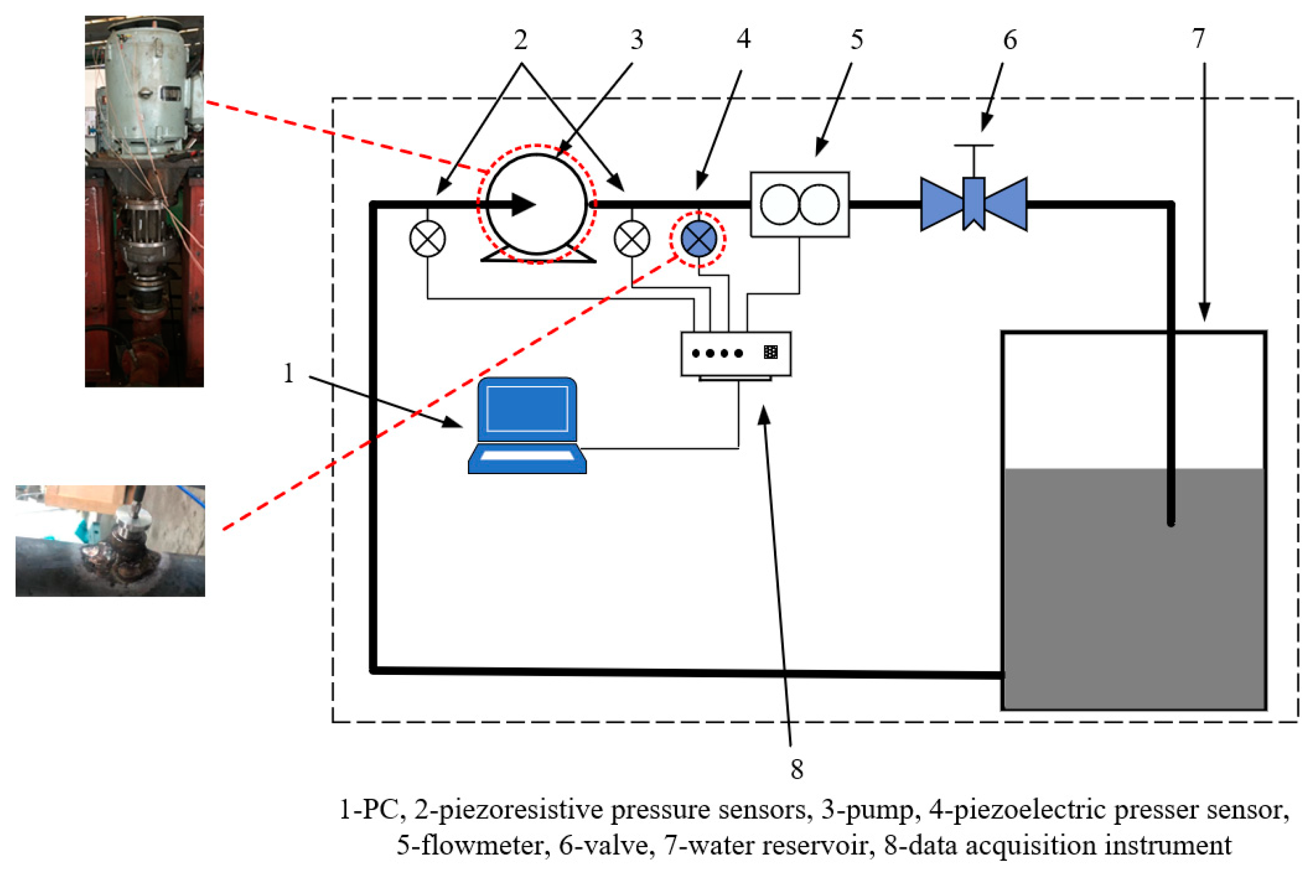
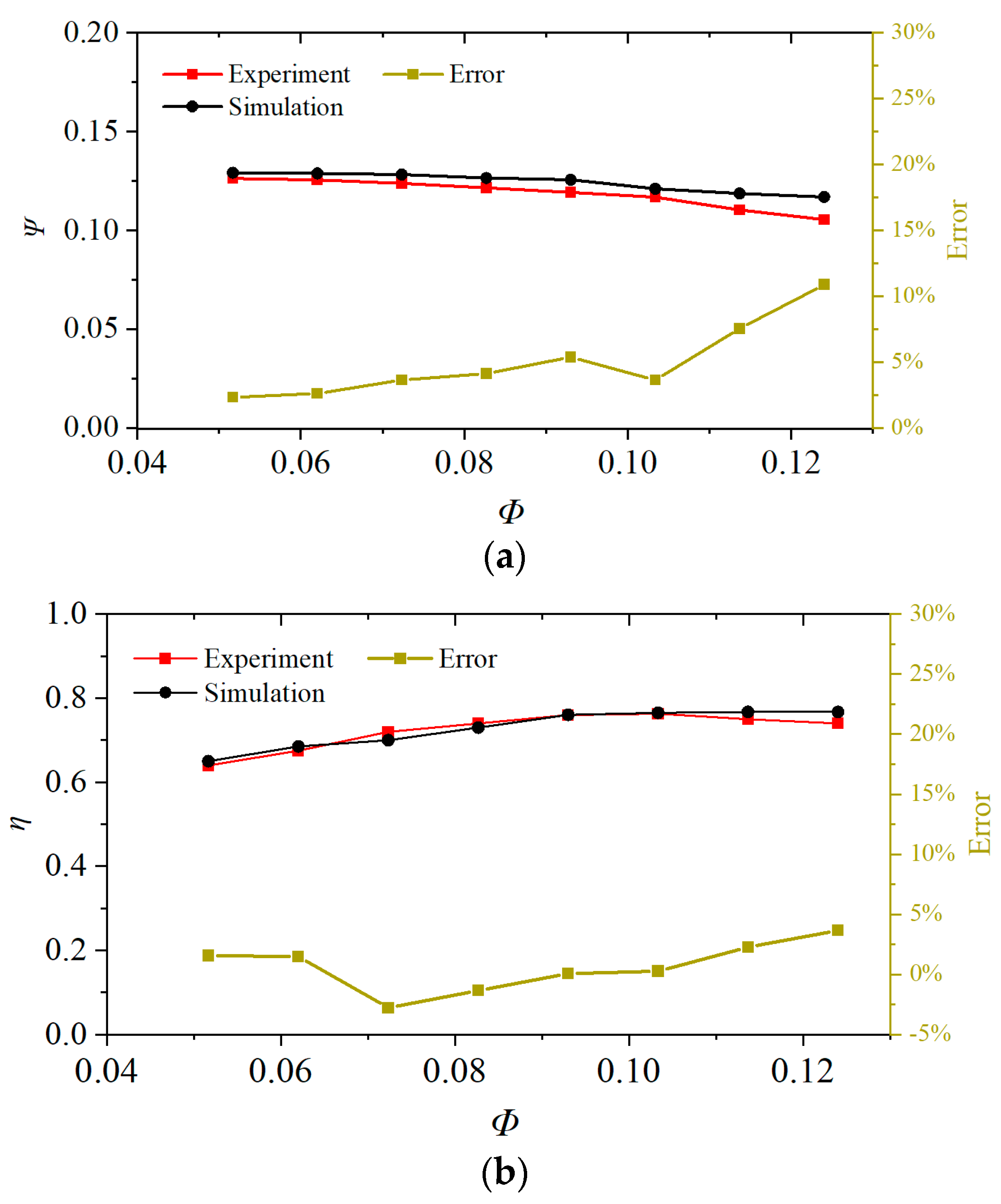
2.4. Experimental Validation

As shown in Figure 6, the hydraulic characteristics of the centrifugal pump were tested in a closed test system. The comparison between the experimental data and simulation results for the hydraulic performance of the centrifugal pump is illustrated in Figure 7a. The head of the pump represents the capacity of the pump to work [40]; it is defined as

$$H=\frac{p_1{-p}_2}{\rho g}+\Delta z,$$

(1)

where $p_2$ is the total pressure at the pump inlet, $p_1$ is the total pressure at the pump outlet, and $\Delta z$ is the height difference between the inlet and outlet of the centrifugal pump. The trends of the pump characteristic curves obtained experimentally and via the simulation are consistent with each other, with an error of only 3.6% at the nominal flow rate.

The dimensionless flow rate $\Phi$ [40], the dimensionless head $\Psi$, and the pressure coefficient $C_P$ can be defined as, respectively:

$$\Phi =\frac{Q}{\omega {D_2}^2{b}_2},$$

(2)

$$\Psi =\frac{gH}{{\omega }^2{D_2}^2},$$

(3)

$$C_P=\frac{p}{0.5\rho {\omega }^2{(D_2/2)}^2}.$$

(4)

Due to the simplifications made to the model and boundary conditions in the simulation, disparities exist between the experimental and simulation results. However, overall, the simulation model reasonably reflects the experimental results.

3. Simulation Strategies

3.1. Flow Governing Equations

In terms of discretization, the finite volume method was employed to solve the three-dimensional control equations governing the incompressible water flow in the model pump. These equations included the mass conservation and the momentum conservation equations. The instantaneous continuity equation and the momentum equation for incompressible fluids are, respectively, as follows:

$$\frac{\partial {\overline{u}}_i}{\partial x_i}=0,$$

(5)

$$\frac{\partial {\overline{u}}_i}{\partial t}+\frac{\partial {\overline{u}}_i{\overline{u}}_j}{\partial x_j}=-\frac{1}{\rho }\frac{\partial p}{\partial x_i}+\frac{1}{\rho }\frac{\partial }{\partial x_j}({\tau }_{ij}-\rho \overline{{u^{\prime }}_i{u^{\prime }}_j}),$$

(6)

where ${\overline{u}}_i$ and ${\overline{u}}_j$ represent the velocity components in the Cartesian coordinate system, p represents the pressure in the fluid field, $\rho$ indicates the density of water, and ${\tau }_{ij}$ represents the shear stress of the fluid parcel.

The relationship between the Reynolds stress and the average velocity gradient, as well as the turbulent viscosity, is governed by the gradient diffusion hypothesis.

$$-\rho \overline{{u^{\prime }}_i{u^{\prime }}_j}=\rho v_T\left(\frac{\partial {\overline{u}}_i}{\partial x_j}+\frac{\partial {\overline{u}}_j}{\partial x_i}\right)-\frac{2}{3}{\delta }_{ij}\rho k,$$

(7)

In the SST k-w model, the turbulent eddy viscosity is represented as

$${\nu }_T=\frac{a_{1}k}{\max (a_1\omega ,S{F}_2)},$$

(8)

k represents the turbulent kinetic energy, which is responsible for the energy within the turbulence. Meanwhile, the dissipation rate $\omega$ can be considered as a variable determining the turbulence scale.

The turbulent kinetic energy k is derived from the following equation, where $\nu$ denotes the viscosity of water:

$$\frac{\partial k}{\partial t}+U_j\frac{\partial k}{\partial x_j}=P_k-{\beta }^{*}k\omega +\frac{\partial }{\partial x_j}\left[\left(\nu +{\sigma }_k{\nu }_T\right)\frac{\partial k}{\partial x_j}\right],$$

(9)

In addition, the equation for the dissipation rate ω is derived using the following formula:

$$\frac{\partial \omega }{\partial t}+U_j\frac{\partial \omega }{\partial x_j}=\alpha S^2-\beta {\omega }^2+\frac{\partial }{\partial x_j}\left[\left(\nu +{\sigma }_{\omega }{\nu }_T\right)\frac{\partial \omega }{\partial x_j}\right]+2(1-F_1){\sigma }_{\omega 2}\frac{1}{\omega }\frac{\partial k}{\partial x_i}\frac{\partial \omega }{\partial x_i}.$$

(10)

Additionally, there are some auxiliary equations and coefficients in the model:

$$F_2=\tanh \left[{\left[\max \left(\frac{2\sqrt{k}}{{\beta }^{*}\omega y},\frac{500\nu }{y^2\omega }\right)\right]}^2\right],$$

(11)

$$P_k=\min \left({\tau }_{ij}\frac{\partial U_i}{\partial x_j},10{\beta }^{*}k\omega \right),$$

(12)

$$F_1=\tanh \left\{{\left\{\min \left[\max \left(\frac{\sqrt{k}}{{\beta }^{\ast }\omega y},\frac{500\nu }{y^2\omega }\right),\frac{4{\sigma }_{\omega 2}k}{C{D}_{k\omega }{y}^2}\right]\right\}}^4\right\},$$

(13)

$$C{D}_{k\omega }=\max \left(2\rho {\sigma }_{\omega 2}\frac{1}{\omega }\frac{\partial k}{\partial x_i}\frac{\partial \omega }{\partial x_i},{10}^{-10}\right),$$

(14)

$$\varphi ={\varphi }_1{F}_1+{\varphi }_2(1-F_1),$$

(15)

where $F_1$ and $F_2$ represent the blending function, and $P_k$ denotes the turbulent kinetic energy production term. The following are the coefficients of the abovementioned parameters: ${\alpha }_1=\frac{5}{9},{\alpha }_2=0.44$, ${\beta }_1=\frac{3}{40},{\beta }_2=0.0828$, ${\beta }^{\ast }=\frac{9}{100}$, ${\sigma }_{k1}=0.85,{\sigma }_{k2}=1$, and ${\sigma }_{\omega 1}=0.5,{\sigma }_{k2}=0.856$.

3.2. Entropy Production Theory

This study introduced the entropy generation theory to quantitatively investigate the impact of the blade trailing edge on the energy loss mechanism in the fluid flow of a centrifugal pump.

During the operational process of adiabatic machinery, irreversible hydraulic losses are generated due to the viscous Reynolds stresses in the boundary layer, as well as secondary flows and backflows within the channel, thereby converting mechanical energy into internal energy. For incompressible fluids such as water, the specific entropy s serves as a state variable and has its own transport or balance equation [9,14]:

$$\rho \left(\frac{\partial s}{\partial t}+u_1\frac{\partial s}{\partial x_1}+u_2\frac{\partial s}{\partial x_2}+u_3\frac{\partial s}{\partial x_3}\right)=-div\left(\frac{\overrightarrow{q}}{T}\right)+\frac{\Phi }{T}+\frac{{\Phi }_{\Theta }}{T^2},$$

(16)

In this equation, $s$ is the specific entropy, and $u_1$, $u_2$, and $u_3$ are the velocities in the three directions of the Cartesian coordinate system. $x_1$, $x_2$, and $x_3$ correspond to the position parameters in the three directions; $\overrightarrow{q}$ is the heat flux density vector; and $T$ is the temperature. The second and third terms on the right-hand side represent the energy losses resulting from the irreversible processes. The second term represents the viscous losses, while the third term represents the heat transfer caused by finite temperature gradients. Due to the incompressibility of the flow, the laminar viscous dissipation functions $\Phi$ and ${\Phi }_{\Theta }$ on the right-hand side are, respectively, simplified and calculated as follows:

$$\begin{array}{l}\Phi =\mu \cdot \left[2\left({\left(\frac{\partial u_1}{\partial x_1}\right)}^2+{\left(\frac{\partial u_2}{\partial x_2}\right)}^2+{\left(\frac{\partial u_3}{\partial x_3}\right)}^2\right)\right.\\ \hspace{1em}\hspace{1em} \left.+{\left(\frac{\partial u_1}{\partial x_2}+\frac{\partial u_2}{\partial x_1}\right)}^2+{\left(\frac{\partial u_1}{\partial x_3}+\frac{\partial u_3}{\partial x_1}\right)}^2+{\left(\frac{\partial u_2}{\partial x_3}+\frac{\partial u_3}{\partial x_2}\right)}^2\right]\end{array}$$

(17)

$${\Phi }_{\Theta }=\lambda \left[{\left(\frac{\partial T}{\partial x_1}\right)}^2+{\left(\frac{\partial T}{\partial x_2}\right)}^2+{\left(\frac{\partial T}{\partial x_3}\right)}^2\right]$$

(18)

In this work, it was assumed that the temperature within the fluid domain remained constant. Consequently, the entropy generation caused by the temperature gradients was neglected. Hence, the third term on the right-hand side of the equation could be ignored. For the turbulent region, the Reynolds-averaged method was adopted, considering the mean and fluctuating terms to describe the instantaneous flow characteristics, entropy components $s=\overline{s}+s\prime$, and velocity components $u_i={\overline{u}}_i+u_i\prime$. Therefore, the entropy transport equation can be simplified as [9]:

$$\begin{array}{lll}\rho \left(\frac{\partial \overline{s}}{\partial t}+\overline{u_1}\frac{\partial \overline{s}}{\partial x_1}+\overline{u_2}\frac{\partial \overline{s}}{\partial x_2}+\overline{u_3}\frac{\partial \overline{s}}{\partial x_3}\right)& =& -\overline{\nabla \cdot \left(\frac{\overrightarrow{q}}{T}\right)}\\ & -& \rho \left(\frac{\partial \overline{u_1^{\prime }{s}^{\prime }}}{\partial x_1}+\frac{\partial \overline{u_2^{\prime }{s}^{\prime }}}{\partial x_2}+\frac{\partial \overline{u_3^{\prime }{s}^{\prime }}}{\partial x_3}\right)+\left(\frac{\overline{\Phi }}{T}\right)\end{array}$$

(19)

$S_{PRO,D\prime }$ is the time-averaged entropy generated by dissipation in turbulence, which includes the direct dissipation $S_{PRO,D}$ and the turbulent dissipation $S_{PRO,D^{\prime }}$. The calculation formula for it is

$$\frac{\overline{\Phi }}{T}=S_{PRO,D}=S_{PRO,\overline{D}}+S_{PRO,D^{\prime }},$$

(20)

$$\begin{array}{l}{S}_{PRO,\overline{D}}=\frac{\mu }{T}·\left[2\left({\left(\frac{\partial {\overline{u}}_1}{\partial x_1}\right)}^2+{\left(\frac{\partial {\overline{u}}_2}{\partial x_2}\right)}^2+{\left(\frac{\partial {\overline{u}}_3}{\partial x_3}\right)}^2\right)+\right.\\ \hspace{1em}\hspace{1em}\hspace{1em}\hspace{1em}\hspace{1em}\left.{\left(\frac{\partial {\overline{u}}_1}{\partial x_2}+\frac{\partial {\overline{u}}_2}{\partial x_1}\right)}^2+{\left(\frac{\partial {\overline{u}}_1}{\partial x_3}+\frac{\partial {\overline{u}}_3}{\partial x_1}\right)}^2+{\left(\frac{\partial {\overline{u}}_2}{\partial x_3}+\frac{\partial {\overline{u}}_3}{\partial x_2}\right)}^2\right],\end{array}$$

(21)

$$\begin{array}{l}{S}_{PRO,D\prime }=\frac{\mu }{T}·\left[2\left(\overline{{\left(\frac{\partial {u_1}^{\prime }}{\partial x_1}\right)}^2}+\overline{{\left(\frac{\partial {u_2}^{\prime }}{\partial x_2}\right)}^2}+\overline{{\left(\frac{\partial {u_3}^{\prime }}{\partial x_3}\right)}^2}\right)\right.\\ \hspace{1em}\hspace{1em}\hspace{1em}\hspace{1em} \left.+\overline{{\left(\frac{\partial {u_1}^{\prime }}{\partial x_2}+\frac{\partial {u_2}^{\prime }}{\partial x_1}\right)}^2}+\overline{{\left(\frac{\partial {u_1}^{\prime }}{\partial x_3}+\frac{\partial {u_3}^{\prime }}{\partial x_1}\right)}^2}+\overline{{\left(\frac{\partial {u_2}^{\prime }}{\partial x_3}+\frac{\partial {u_3}^{\prime }}{\partial x_2}\right)}^2}\right],\end{array}$$

(22)

The solution of $S_{PRO,D^{\prime }}$ is non-closed due to the absence of corresponding parameters in the solving process. This can be addressed by using the method proposed by Kock et al. [42] to calculate the entropy source of turbulent dissipation. The calculation formula is expressed by

$$S_{PRO,D^{\prime }}={\beta }^{*}\frac{\rho \omega k}{\overline{T}},$$

(23)

where the value of ${\beta }^{*}$ is 0.09. By integrating $S_{PRO,D}$ corresponding to the fluid domain, the total entropy yield $S_{PRO}$ generated by the viscous dissipation effect in the fluid domain can be obtained as

$$S_{PRO}={\int }_V{S}_{PRO,\overline{D}}dV+{\int }_V{S}_{PRO,D^{\prime }}dV.$$

(24)

3.3. Dynamic Mode Decomposition

Before applying the DMD method to analyze the data, the flow field data obtained from the numerical simulation was preprocessed into a continuous snapshot form with a constant time step $\Delta t$ in the form of vectors. Each vector at each snapshot is denoted as $x_i$, and they are arranged into matrices $X_1$ and $X_2$, where N represents the total number of snapshots.

$$X_1=\{x_1,x_2,x_3,\dots ,x_N\},$$

(25)

$$X_2=\{x_2,x_3,x_4,\dots ,x_{N+1}\},$$

(26)

Assuming that any two consecutive snapshot data points satisfy a linear transformation matrix $A$, $X_2$ can be represented as

$$X_2=A{X}_1.$$

(27)

The dynamic characteristics of the flow system can be represented by the time evolution matrix $A$. $X_2$ can then be expressed as

$$X_2=[A{x}_0,A{x}_1,\dots A{x}_{N-1}]={AX}_1.$$

(28)

The eigenvalues and eigenvectors of A can be computed through the following steps. First, $X_1$ can be written using a singular value decomposition (SVD) as follows:

$$X_1=U\mathsf{\Sigma }{V}^{\mathrm{H}},$$

(29)

where the first r columns of the matrix $U$ and $V$ can be truncated through SVD, and the first r rows and columns of $\mathsf{\Sigma }$ are sorted in a descending order by the singular values to obtain $U_r$, ${\mathsf{\Sigma }}_r$, and $V_r$.

$$Y=U_r^{T}A{U}_r=U_r^{T}X{V}_r{\mathsf{\Sigma }}_r^{-1}\in R^{r\times r}.$$

(30)

Second, the eigenvalues and eigenvectors for Y can be found as follows:

$$Y{\nu }_j={\mu }_j{\nu }_j,$$

(31)

where ${\mu }_j$ is the eigenvalue of $Y$ and ${\nu }_j$ is the corresponding eigenvector of $Y$.

Each non-zero ${\mu }_j$ serves as a DMD eigenvalue, and the corresponding DMD mode is expressed by

$$v_i={\mu }_i^{-1}X{V}_r{\mathsf{\Sigma }}_r^{-1}{\nu }_i.$$

(32)

The relationship of the eigenvalues is

$${\lambda }_j=1/\mathsf{\Delta }\mathrm{t}\log ({\mu }_j).$$

(33)

Therefore, by examining the real and imaginary parts of ${\lambda }_j$, the growth or decay rate and the frequency of the DMD modes can be obtained.

4. Results and Discussion

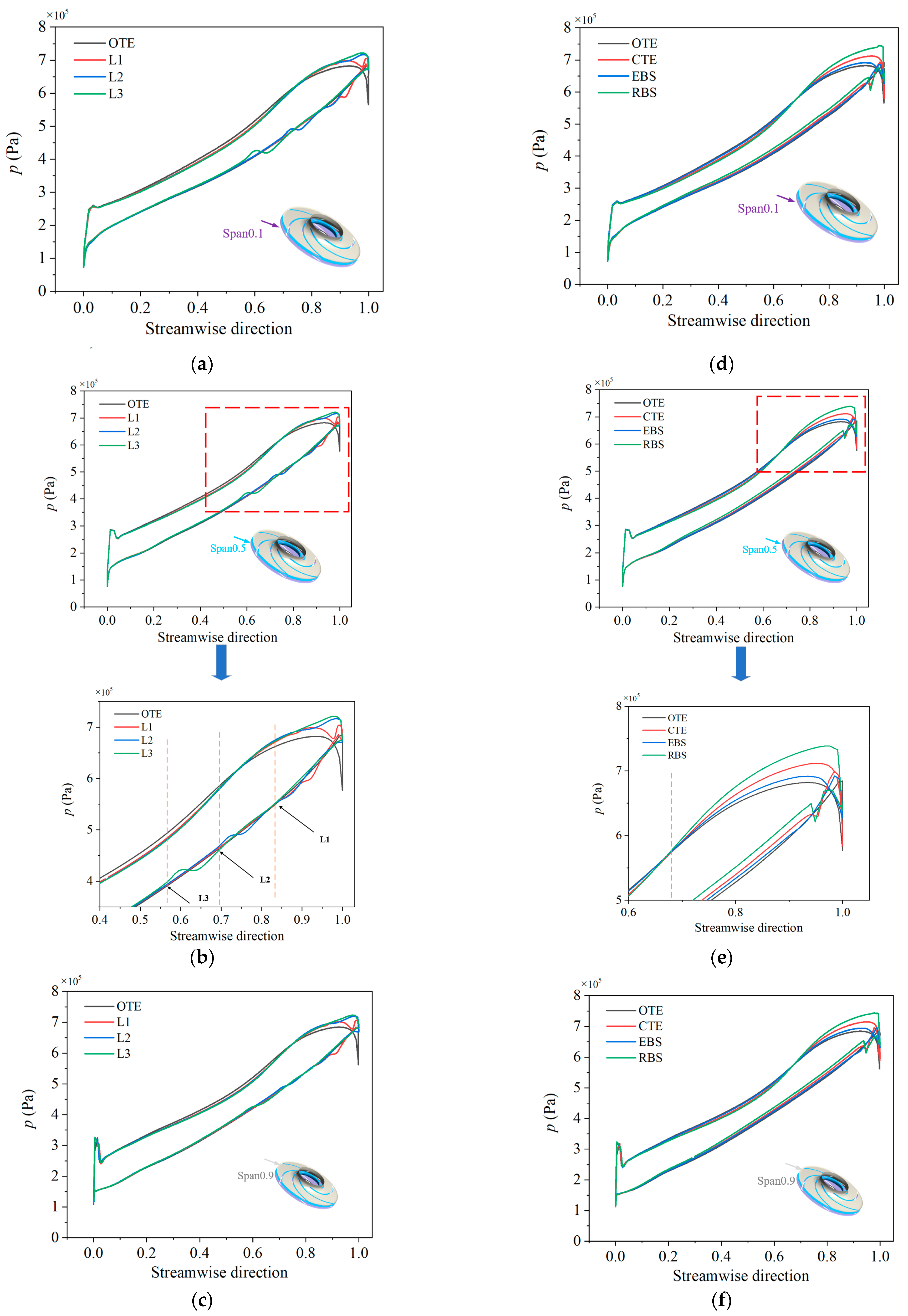
4.1. Blade Pressure Distribution

Figure 8 presents the static pressure distributions of blades with different outlet angles and different blade trailing edge shapes at the same span positions (0.1, 0.5, and 0.9). The trailing edge shape has varying degrees of influence on the pressure distribution across different spans. The abscissa represents the streamline position, with the coordinates normalized to values between 0 and 1, from the leading edge to the trailing edge. In the figure, two lines indicate a gradual increase in pressure from the leading edge to the trailing edge, where the upper side corresponds to the pressure side and the lower side to the suction side.

In Series 1, changes in the outlet angle of the trailing edge mainly affect the pressure load of the suction surface. Because of the different outlet angles, the pressure on the suction surface of Series 1 fluctuates. With a large outlet angle, the pressure in the streamwise direction of the trailing edge begins to fluctuate earlier. The pressure in L3 starts to fluctuate at 0.55 along the streamwise direction, the pressure in L2 starts to fluctuate at 0.70 along the streamwise direction, and the pressure in L1 starts to fluctuate at 0.83 along the streamwise direction.

In Series 2, changes in the trailing edge primarily affect the loading distribution at the rear edge of the blade, with a more pronounced impact on the pressure side compared to the suction side. The pressure at the trailing edge is significantly higher for the RBS shape than for the other three shapes. The pressure load begins to change at 0.665 along the streamwise direction at a 0.5 span. The peak value of the RBS pressure load is the largest, while that of the OTE is the smallest, with a difference of 9.688 × 10⁴ Pa.

The analysis above suggests that both the angle and shape of the trailing edge affect the pressure distribution on the blade surface. This, in turn, influences the loading distribution of the pump blades and subsequently impacts the performance of the pump.

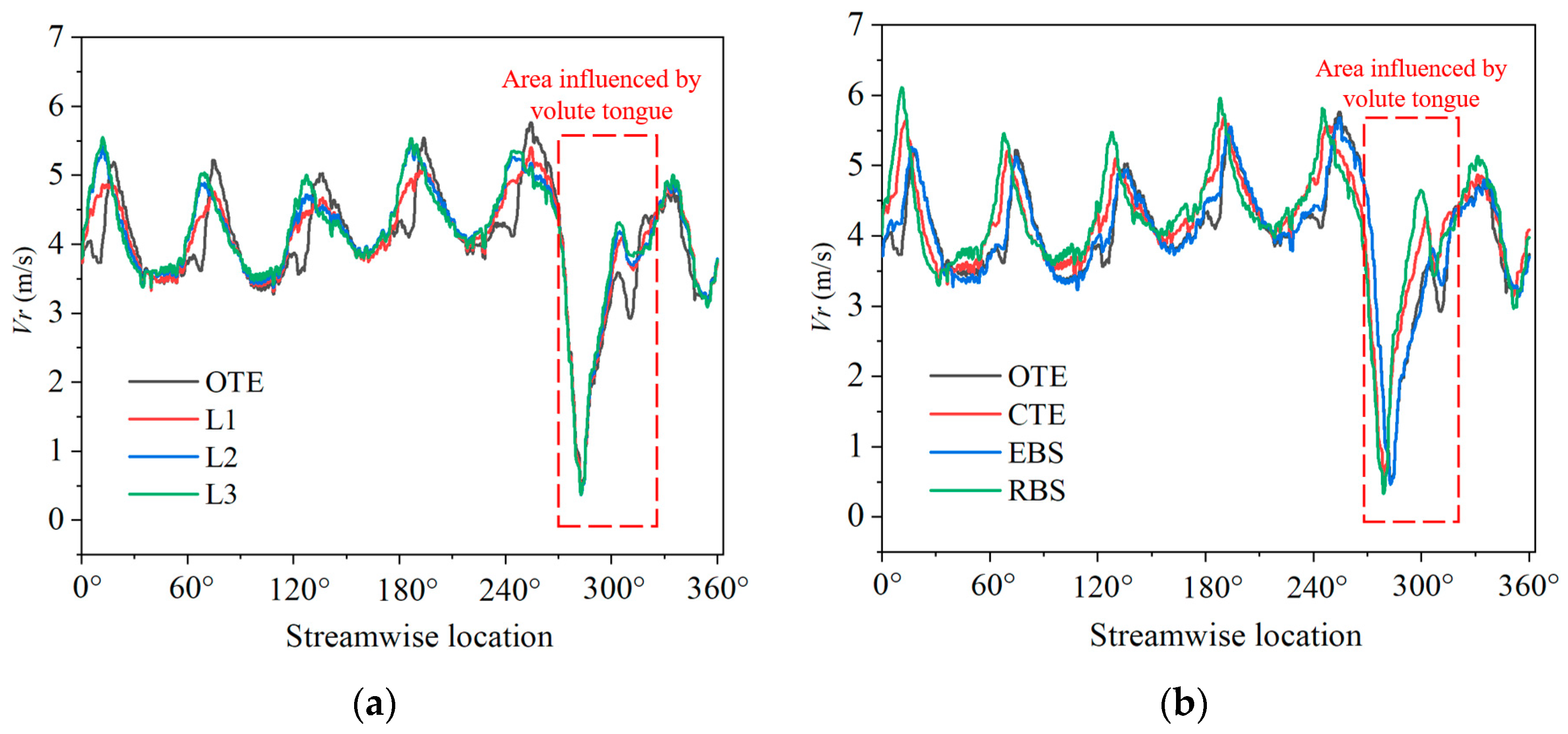
4.2. Circumferential Velocity Distribution at the Impeller Outlet

As shown in Figure 9a, in order to examine the uniformity of the radial velocity distribution at the exit of the impeller, monitoring points were arranged circumferentially within the volute region (yellow circle), and the rotation direction of the pump is marked (red arrow). The position at 0° was designated as the area where the liquid begins to converge in the volute. Figure 10a,b present a comparison of the radial velocity ($V_r$) at the impeller exit for Series 1 and Series 2, respectively. Evidently, the 285° position, corresponding to the location of the volute tongue, demonstrates the most rapid decrease in velocity. In the transient one-revolution velocity distribution at this position, the radial velocity initially increases and then decreases, exhibiting fluctuations based on the position. In addition to the region affected by the volute tongue, six velocity peaks are observed, indicating the positions of the pressure side jets.

In Figure 10a, it can be observed that the peak increases with the magnitude of the angle after the direction of the trailing edge is changed. Figure 10b shows a similar general trend of the radial velocity distribution when the trailing edge shape is altered, but with a shift in the position of the trailing edge peak. The change in the direction of the blade exit velocity is influenced by changes in the pressure and suction sides, which in turn affect the peak positions where the velocities intersect. The peak positions for the OTE and EBS shapes remain mostly the same, while those for the CTE and RBS shapes shift to the left, with the RBS shape exhibiting the most significant peak.

In order to quantitatively describe the uniformity of the radial velocity distribution at the exit, $V_r^{*}$, certain parameters were introduced, as follows:

$$V_r^{*}=\sqrt{\frac{1}{N}{\displaystyle \sum _{n=1}^N{\left(V_r-{\overline{V}}_r\right)}^2}},N=300,$$

(34)

where ${\overline{V}}_r$ is the spatial circumferential velocity obtained after subtracting the mean value of the points in the area influenced by the volute tongue. The calculation results are shown in

Table 3. Values for the different trailing edge shapes.

Trailing Edge Type	${\mathit{V}}_{\mathit{r}}^{*}$
OTE	14.2
L1	12.57
L2	13.46
L3	13.89
CTE	14
EBS	14.2
RBS	15.36

.

It can be seen that an increase in the exit angle in Series 1 leads to a higher degree of non-uniformity in $V_r^{*}$. In Series 2, the RBS shape exhibits the largest degree of radial velocity heterogeneity, which is 8.2% larger compared to the OTE shape. On the other hand, the CTE shape exhibits the smallest degree of radial velocity heterogeneity, which is 1.4% smaller compared to the OTE shape.

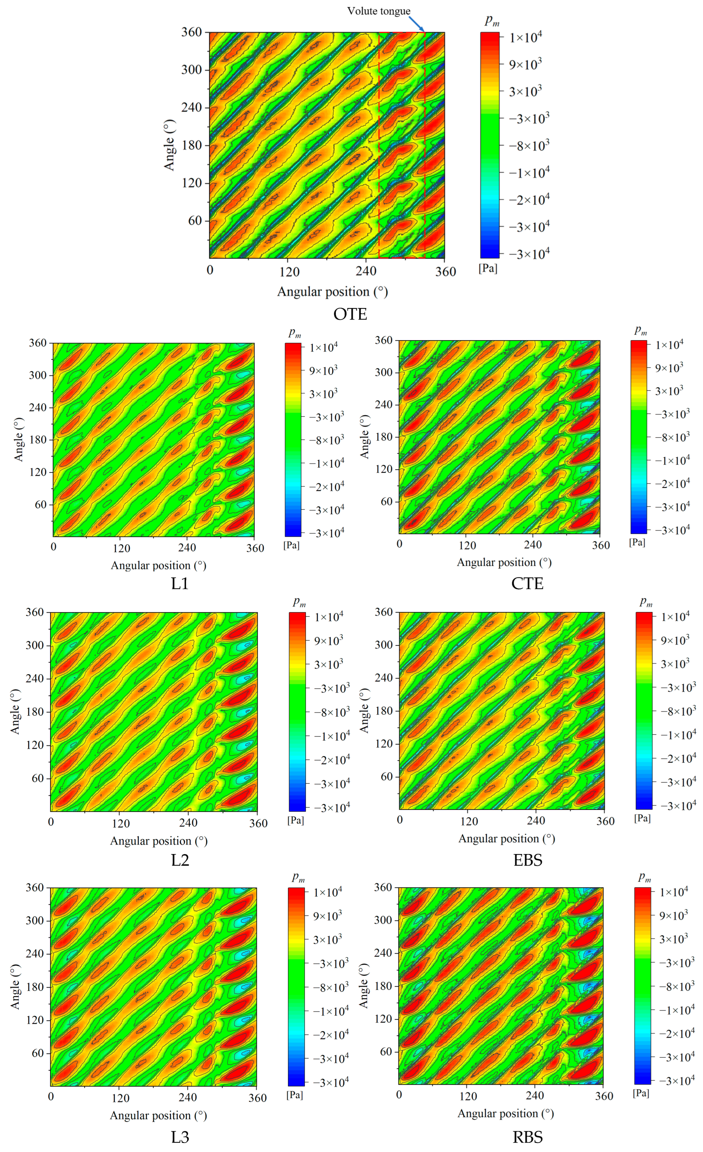
4.3. Spatio-Temporal Analysis of the Pressure Flow Field at the Impeller Outlet

In order to clearly observe the spatio-temporal distribution characteristics of the outlet pressure, $p_m$, a variable analysis was performed:

$$\overline{p}=\frac{1}{N}\sum _{n=1}^{N}p,N=360,$$

(35)

$$p_m=p-\overline{p},$$

(36)

where the mean pressure, $\overline{p}$, is the average value at a certain measurement point over one complete revolution of the impeller. $p_m$ is selected as a reference value, which is the pressure value of a single monitoring point minus $\overline{p}$.

Figure 11 shows the dynamic changes in the pressure near the impeller outlet, offering insights into the temporal and spatial characteristics of the instantaneous pressure, excluding the mean value. The abscissa, which represents the angular position shown in Figure 9, provides a comprehensive view of how the pressure evolves with the position, while the ordinate provides a clear representation of pressure fluctuations over time.

Observing the pressure distribution for the OTE shape, it is evident that the fluctuations follow a periodic pattern both spatially and temporally. Six distinguishable regions of high and low pressure can be observed, progressing as the impeller rotates circumferentially. Notably, the most substantial variations in pressure occur in the vicinity of the volute tongue, indicating the significant influence of this area on the overall pressure dynamics.

In Series 1, the fluctuation amplitude of the pressure gradually increases as the angle at both ends of the trailing edge increases. In Series 2, the fluctuation amplitude of the RBS shape surpasses that of other shapes, suggesting a more pronounced dynamic pressure environment in this shape.

4.4. Entropy Generation Rate Analysis

To quantitatively analyze the changes in energy loss inside the pump after the modification of the trailing edge, entropy generation rate analysis was introduced.

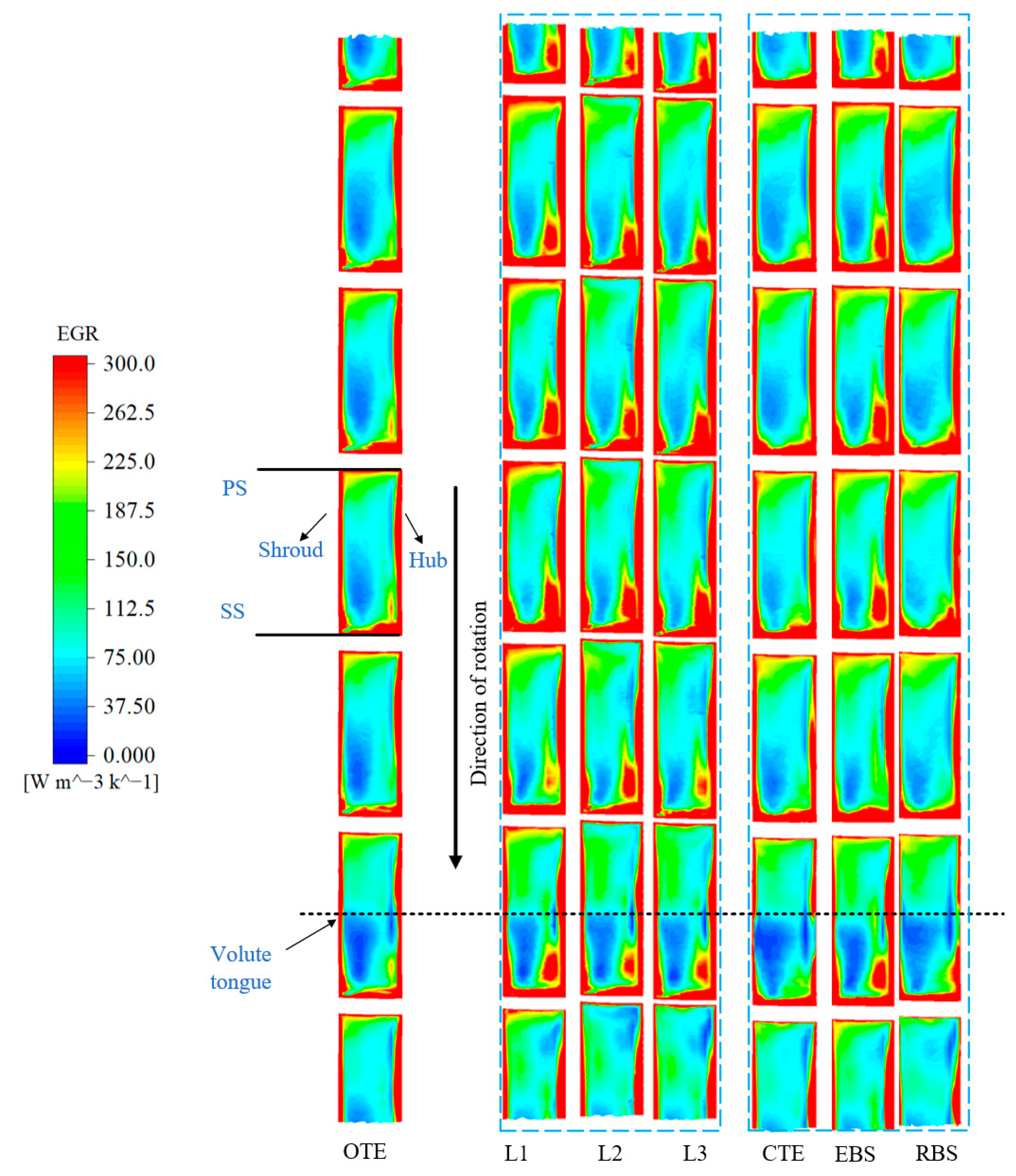
4.4.1. EGR Distribution at the Impeller Outlet

Axial cross-sectional analyses were performed along the impeller radius at R = 0.115 m. Six segments (colored in orange) were designated as entropy generation rate (EGR) monitoring surfaces along the circumferential direction, as illustrated in Figure 12. EGR distribution maps for different types of trailing edges were generated, as shown in Figure 13. In the OTE shape, the locations of the pressure and suction sides were identified. It was observed that $S_{PRO}$ is relatively higher near the wall surface but decreases towards the suction side and the shroud direction. For Series 1, despite a change in the exit angle of the trailing edge, the $S_{PRO}$ values are relatively similar in all six impeller outlet channels. In comparison to the other shapes of Series 2, the EBS shape exhibits additional high $S_{PRO}$ regions near the suction side and the hub direction.

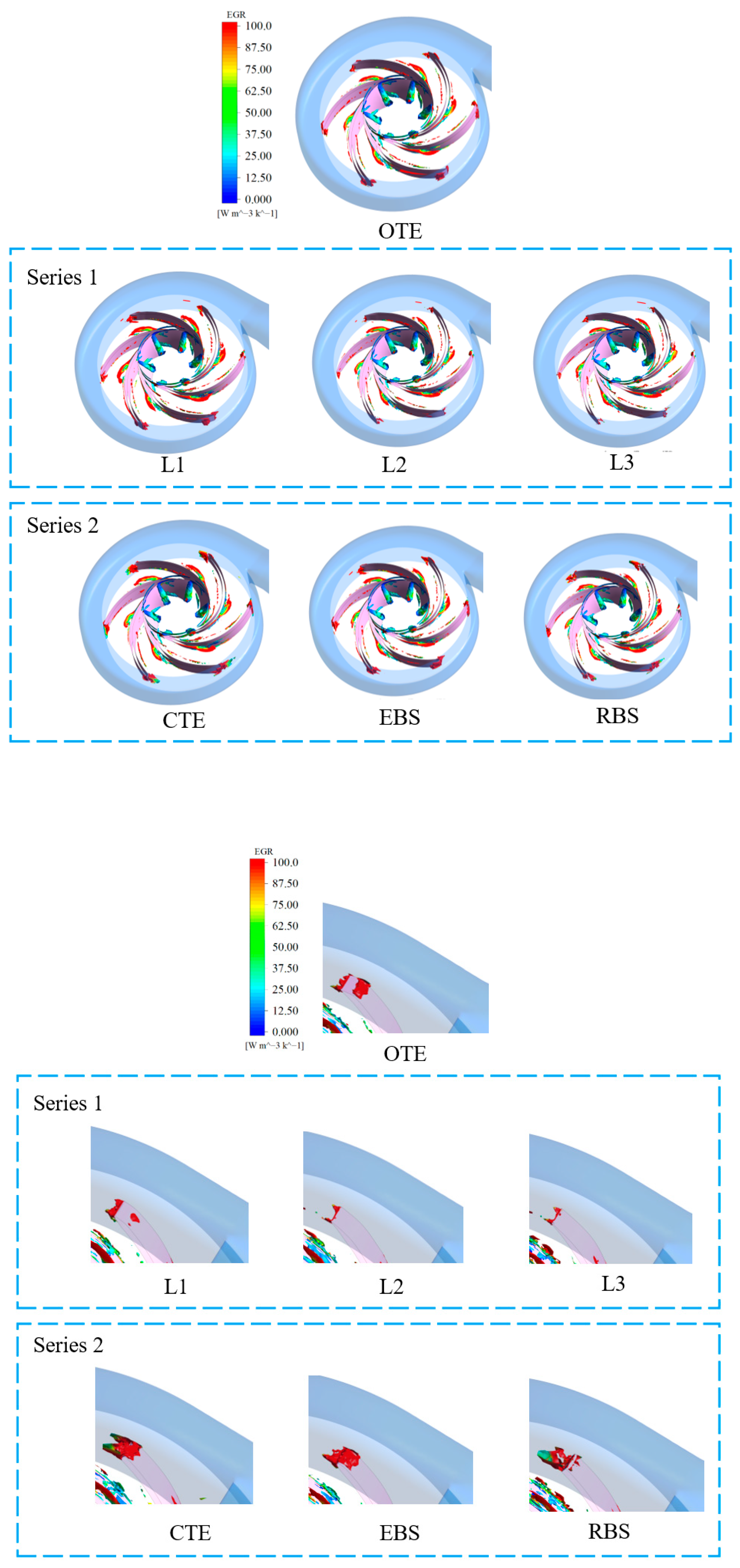
4.4.2. Vortex Distribution at the Trailing Edges

To enable a more comprehensive examination of the energy losses in the wake region, vortex identification was performed in the impeller domain. The first and second generations of the vortex identification methods are capable of detecting the transition of the shear layer disturbance into a vortex cluster; however, they require a threshold value that significantly impacts the visualization of the vortex structure. In contrast, the $\Omega$ method, which represents the latest generation of the vortex identification methods, introduces the novel concept of further decomposing vorticity into rotating and non-rotating parts for the first time [43]. This method incorporates a normalized threshold ranging from 0 to 1, allowing for the visualization of both strong and weak vortex nuclei. The core formula for calculating $\Omega$ is as follows:

$$\begin{array}{l}a={\left(\frac{\partial u_1}{\partial x_1}\right)}^2+\frac{1}{2}{\left[\left(\frac{\partial u_1}{\partial x_2}\right)+\left(\frac{\partial u_2}{\partial x_1}\right)\right]}^2+{\left(\frac{\partial u_2}{\partial x_2}\right)}^2\\ \hspace{1em}\hspace{1em}+\frac{1}{2}{\left[\left(\frac{\partial u_1}{\partial x_3}\right)+\left(\frac{\partial u_3}{\partial x_1}\right)\right]}^2+{\left(\frac{\partial u_3}{\partial x_3}\right)}^2+\frac{1}{2}{\left[\left(\frac{\partial u_2}{\partial x_3}\right)+\left(\frac{\partial u_3}{\partial x_2}\right)\right]}^2,\end{array}$$

(37)

$$b=\frac{1}{2}{\left[\left(\frac{\partial u_1}{\partial x_2}\right)-\left(\frac{\partial u_2}{\partial x_1}\right)\right]}^2+\frac{1}{2}{\left[\left(\frac{\partial u_1}{\partial x_3}\right)-\left(\frac{\partial u_3}{\partial x_1}\right)\right]}^2+\frac{1}{2}{\left[\left(\frac{\partial u_2}{\partial x_3}\right)-\left(\frac{\partial u_3}{\partial x_2}\right)\right]}^2,$$

(38)

$$\begin{array}{ll}Q=& -\frac{1}{2}\left[{\left(\frac{\partial u_1}{\partial x_1}\right)}^2+{\left(\frac{\partial u_2}{\partial x_2}\right)}^2+{\left(\frac{\partial u_3}{\partial x_3}\right)}^2\right]\\ & -\left[\left(\frac{\partial u_1}{\partial x_2}\right)\left(\frac{\partial u_2}{\partial x_1}\right)\right]-\left[\left(\frac{\partial u_1}{\partial x_3}\right)\left(\frac{\partial u_3}{\partial x_1}\right)\right]-\left[\left(\frac{\partial u_2}{\partial x_3}\right)\left(\frac{\partial u_3}{\partial x_2}\right)\right],\end{array}$$

(39)

$$\Omega =\frac{b}{a+b+1/500\times Q}.$$

(40)

The examination of the vortex core distribution on the isosurface reveals a discernible correlation between the shape of the EGR peak region and the distribution of the vortex cores. Figure 14 shows the internal structure of the impeller, which clearly indicates the passage vortex at the blade wall angle and the trailing edge vortex. In Series 1, the angle on both sides of the trailing edge increases, resulting in a reduced vortex structure at the trailing edge. In Series 2, the trailing edge vortex manifests throughout the entirety of the blade’s trailing section for the CTE and EBS shapes, whereas for the OTE shape, the vortex is confined solely to the pressure and suction sides.

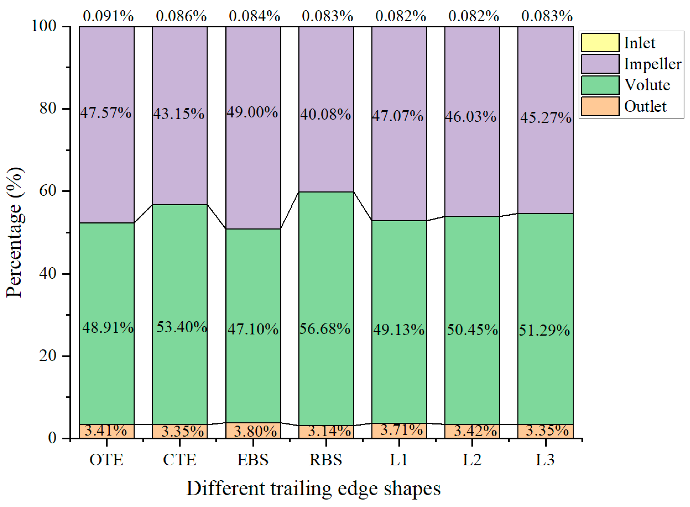
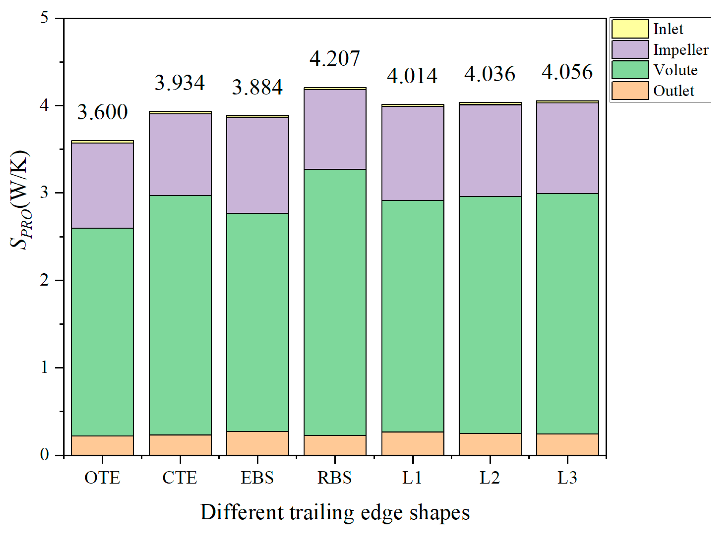
4.4.3. EGR Analysis of the Different Components

Averaging $S_{PRO}$ within each component and representing this value as a percentage graph, as shown in Figure 15, reveal that $S_{\overline{PRO}}$ is primarily generated within the impeller and the volute. The calculation formula for $S_{\overline{PRO}}$ is as follows:

$$S_{\overline{PRO}}=\frac{1}{V}\left(\underset{V}{\int }{S}_{PRO,\overline{D}}dV+\underset{V}{\int }{S}_{PRO,D^{\prime }}dV\right).$$

(41)

For Series 1, with an increase in the exit angle of the trailing edge on both sides, $S_{\overline{PRO}}$ diminishes within the impeller domain but increases within the volute domain. For Series 2, both the CTE and RBS shapes exhibit a relatively higher average EGR within the volute.

Figure 16 shows the total amount of $S_{PRO}$ at different trailing edges. It is evident that variations in the trailing edge predominantly affect $S_{PRO}$ within the volute region. In Series 1, the value of $S_{PRO}$ exhibits a slight change with the change in the exit angle of the trailing edge. In Series 2, the RBS shape exhibits a 16.7% higher $S_{PRO}$ value compared to the OTE shape.

Figure 17 and Figure 18 display a comparison of the dimensionless head of the pump ($\Psi$) and efficiency ($\eta$) for the different trailing edge designs. In Series 1, as the exit angle of the trailing edge increases, the head of the centrifugal pump gradually increases, while the efficiency remains relatively unchanged. In Series 2, changes in the trailing edge shape lead to either a high head and low efficiency or a low head and high efficiency. The efficiency is enhanced by 1.18% with the EBS shape compared to the OTE shape. In future works, the best efficiency point of the pump for different trailing edges should be found under different flow conditions.

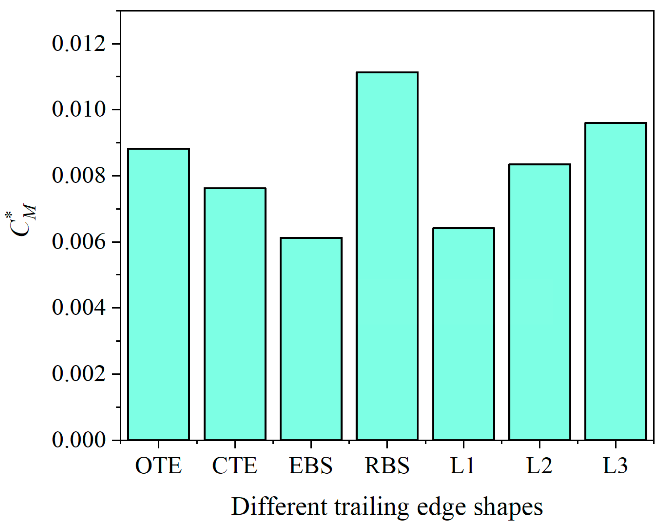
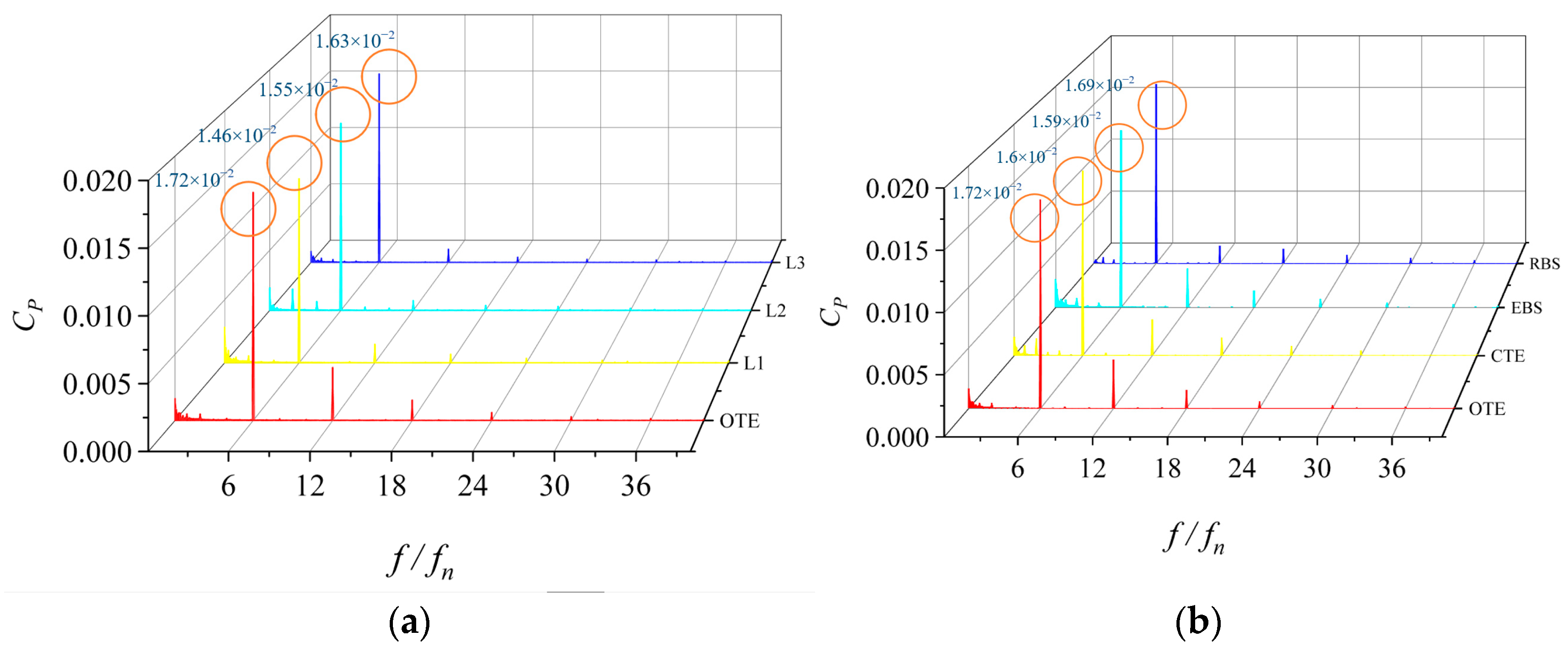
4.5. Pressure Pulsation Analysis of the Pump

Based on the EGR analysis conducted above, it can be seen that the entropy production is largest in the volute. Therefore, monitoring points were set up in the volute domain to analyze pressure fluctuations in the volute under different trailing edges.

As shown in Figure 19, the pressure at the volute tongue fluctuates under the designed flow rate. The rotor–stator interaction in the centrifugal pump results in six distinctive peaks and troughs per cycle. In Series 1, as the exit angle of the trailing edge increases, the pressure fluctuation gradually increases. In Series 2, the EBS shape exhibits notably minimal pressure fluctuations compared to the other shapes. Because the curvatures of CTE and L1 at the trailing edge are greater compared to other shapes, an additional pressure pulsation peak is observed at the volute tongue during each rotation period.

$C_M^{*}$ is introduced as a normalized value to measure the pressure pulsation intensity. It is calculated as follows:

$$\overline{C_P}=\frac{\overline{p}}{0.5\rho {\omega }^2{(D_2/2)}^2},$$

(42)

$$C_M=C_{\mathrm{P}}-\overline{C_{\mathrm{P}}},$$

(43)

$$C_M^{*}=\sqrt{\frac{1}{N}{\displaystyle \sum _{n=1}^N{\left(C_p-{\overline{C}}_p\right)}^2}},N=360,$$

(44)

where $\overline{C_P}$ is the mean pressure coefficient and $C_M$ is the pressure coefficient obtained by subtracting the mean component from the pressure.

Figure 20 provides a comprehensive overview of the pressure fluctuation intensities at the monitoring points ranging from v1 to v8 within the volute region considering different trailing edge shapes. Among all the monitoring points, v4 exhibits the smallest pressure pulsation intensity.

In Series 1, the pressure pulsation intensity follows a consistent distribution law. The points ranging from v2 to v8 exhibit the largest pulsation with the L3 shape and the smallest pulsation with the L1 shape. Only at point v1 does the pulsation distribution show the opposite trend. In Series 2, the OTE shape demonstrates the maximum pressure pulsation intensity at point v1, while the CTE shape exhibits the maximum intensity at point v8. The pressure pulsation intensity of the EBS shape is at its maximum at point v1 and that of the RBS shape is at its maximum at point v8.

The pressure fluctuation intensity distribution at the volute tongue shown in Figure 21 is consistent with that depicted in Figure 19.

To analyze the pressure fluctuations at the volute outlet, a fast Fourier transform is performed on the pressure pulse at the volute exit to obtain its spectrum. The amplitude at the exit represents the blade passing frequency (BPF, 300 Hz) and its harmonics. The spectral analysis, shown in Figure 22a, reveals that the BPF amplitudes of the L1, L2, and L3 shapes show a regular increasing distribution. As depicted in Figure 22b, the OTE shape exhibits the highest amplitude for the BPF among the various trailing edge shapes, while the EBS shape displays the lowest amplitude. The BPF amplitude of the EBS shape is 5.3% smaller than that of the OTE shape.

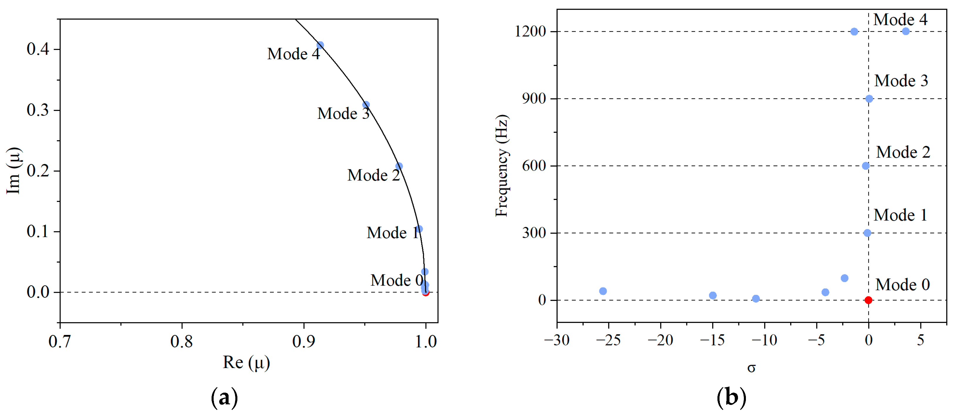
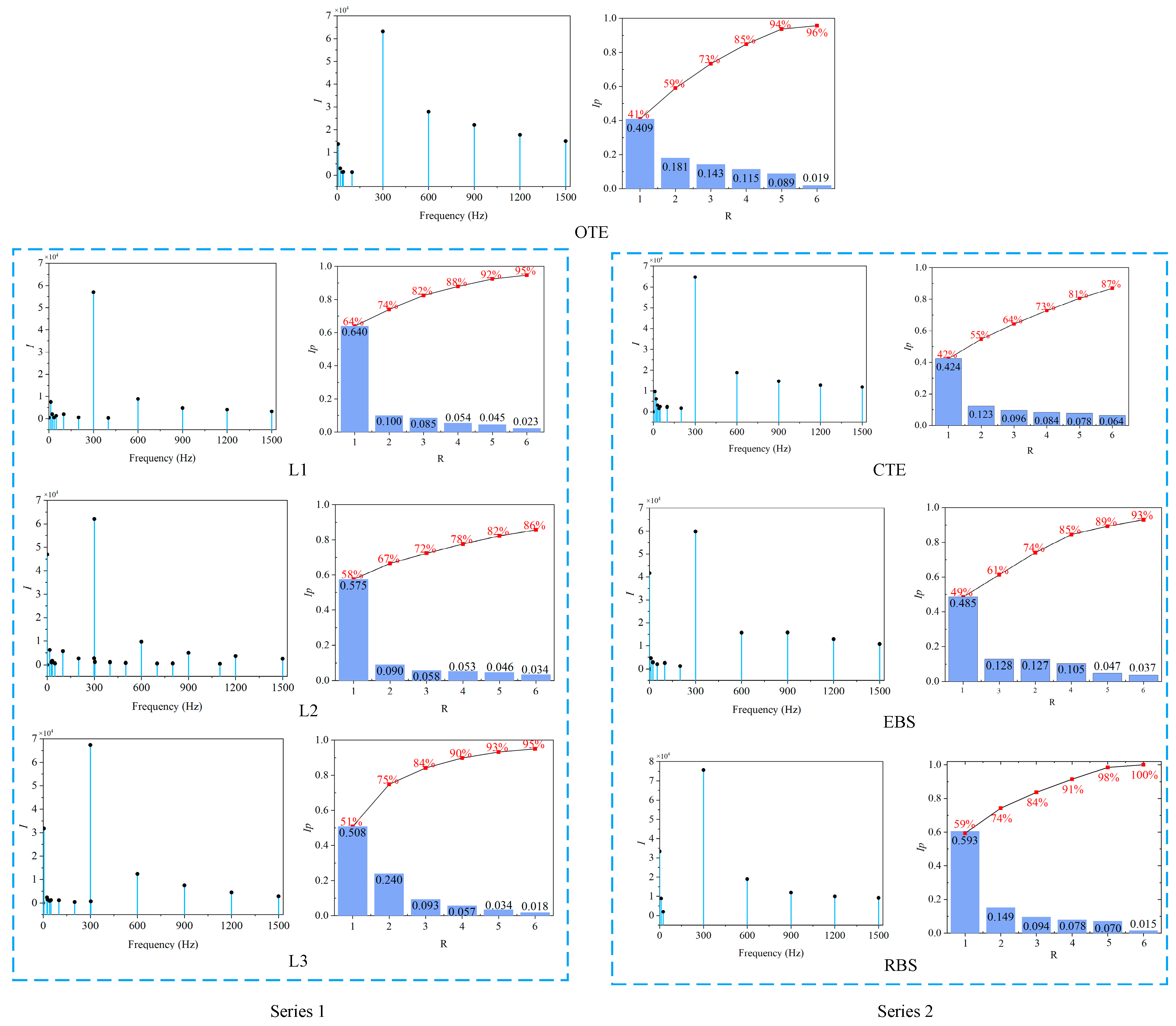
4.6. Dynamic Mode Decomposition in the Volute

The pressure pulse analysis revealed periodic fluctuations in the pressure and velocity fields at the volute. In this section, to determine the dynamic flow characteristics of the unsteady flow field, the pressure data at the volute were used for DMD analysis.

Figure 23a shows the distribution of the eigenvalues of the DMD mode on the complex plane. Based on the results and the physical meaning of the eigenvalues, it can be seen that the eigenvalues of the first four modes are all distributed on the unit circle. Therefore, these modes represent stable flow structures, that is, they do not grow or decay with time. The frequencies and growth rates of different modes are shown in Figure 23b. The growth rates of Modes 1, 2, and 3 corresponding to BPF, 2BPF, and 3BPF, are close to 0.

Figure 24 shows the pressure field for Mode 0. Mode 0 corresponds to zero frequency and reflects the average information of the flow field. The pressure is the greatest at the volute tongue.

The significance of the different modes for the flow field can be evaluated using modal energies. Figure 25 shows the energy distribution characteristics of the DMD modes at different trailing edges, where I_p is the modal energy proportion and R is the order. The bar graph (blue columns) represents the energy proportion of mode i to the total energy, while the dotted line (black arc) graph represents the energy proportion of the first i order mode to the total energy (Mode 0 is not considered).

It can be observed that the BPF and its harmonic frequencies play a dominant role. The flow field formed by Mode 1 is caused by the BPF, and the flow field formed by Mode 2 is caused by the 2BPF. The modal energy of Mode 1 accounts for the largest proportion of the total energy. The modal energy attenuates for Modes 2–5. The sum of the energy proportions of the first four modes is more than 70% of the total modal energy. Modes 1–4 are the main oscillation modes causing an unstable flow in the pump.

For Series 1, the proportion of the first-order mode of the total modes shows a decreasing trend in shapes L1, L2, and L3. For Series 2, the first-order mode of the RBS shape accounts for the largest proportion of the total modes. The RBS shape exhibits a higher proportion compared to other shapes.

Figure 26 illustrates the evolution of the pressure amplitude with time in the first-order and second-order modes at different trailing edge volute tongues after DMD.

In Mode 1, the pressure pulsation amplitude is the smallest for the L3 shape and the largest for the L1 shape in Series 1. In Series 2, the pressure pulsation amplitude is the largest for the RBS shape and the smallest for the EBS shape. In Mode 2, the pulsation amplitudes of Series 1 are consistent with those in Mode 1, while the OTE shape exhibits the largest pulsation amplitude and the EBS shape displays the smallest pulsation amplitude in Series 2.

Figure 27 shows the pressure profiles for Modes 1 and 2. The modal pressure field within the volute can be observed. The high- and low-pressure areas alternate, and the modal pressure field has different effects at different circumferential positions.

Figure 28 illustrates the evolution of pressure fluctuations at spatial positions under Modes 1 and 2 considering the different trailing edge shapes. In Series 1, there are six peaks and troughs in the circumferential spatial distribution. Decreasing the angle of the trailing edge causes the peak value in Mode 1 to shift towards the direction of the impeller rotation and considerably reduces the amplitude of Mode 2. In Series 2, the RBS shape exhibits a more uneven distribution compared to the OTE shape in Mode 1. However, its amplitude for Mode 2 is smaller than that of the OTE shape. Nevertheless, since Mode 1 is the main mode, the total amplitude of the RBS shape is ultimately more uneven.

The modal space inhomogeneity, MSI, is defined as

$$MSI=\sqrt{\frac{1}{N}{\displaystyle \sum _{n=1}^N{\left(C_p^{\prime }-{\overline{C}}_p^{\prime }\right)}^2}},N=360,$$

(45)

where $C_p^{\prime }$ and ${\overline{C}}_p^{\prime }$ are the normalized pressure and the normalized average pressure at the circumferential position in different modes, respectively. The calculation results are shown in

Table 4. MSI values for the different trailing edge shapes.

Trailing Edge Type	MSI of Mode 1	MSI of Mode 2
OTE	0.1037	0.0697
L1	0.0911	0.019
L2	0.1022	0.021
L3	0.1139	0.0286
CTE	0.1063	0.0441
EBS	0.096	0.0346
RBS	0.1323	0.0443

.

In Series 1, as the exit angle on both sides of the trailing edge increases, the modal space inhomogeneity exhibits an initial decrease followed by an increase in Mode 1. The trend in Mode 2 is consistent with that in Mode 1. In Series 2, the modal space inhomogeneity of the RBS shape is the largest, being 27% greater than that of the OTE shape in Mode 1. On the other hand, it is 7.4% smaller for the EBS shape compared to the OTE shape. Changes to the trailing edge shape have little effect on Mode 2. The MSI value in Mode 1 is essentially consistent with the pressure fluctuation analysis conducted earlier.

5. Conclusions

By combining accurate numerical calculation methods and flow analysis techniques, this study investigated the unsteady flow structures and pressure pulsation characteristics of a centrifugal pump. The influence of different trailing edges on the unsteady flow in the pump was analyzed by entropy generation rate analysis and the DMD method. The following conclusions were drawn:

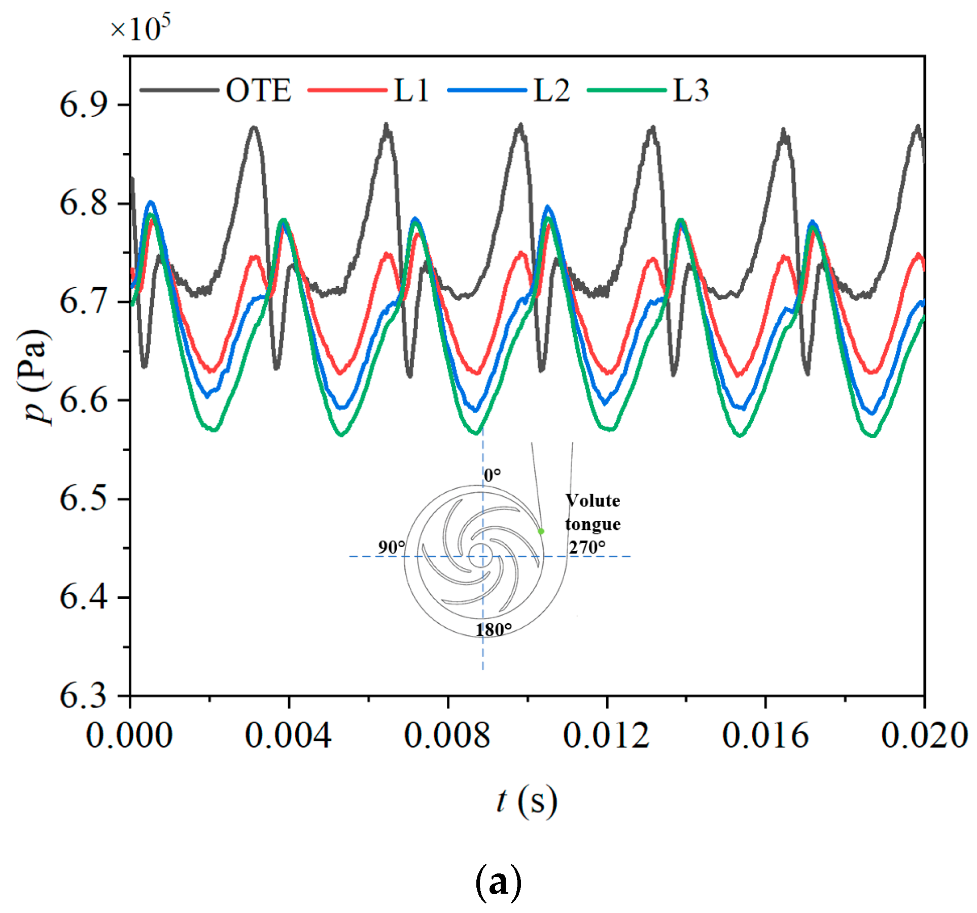
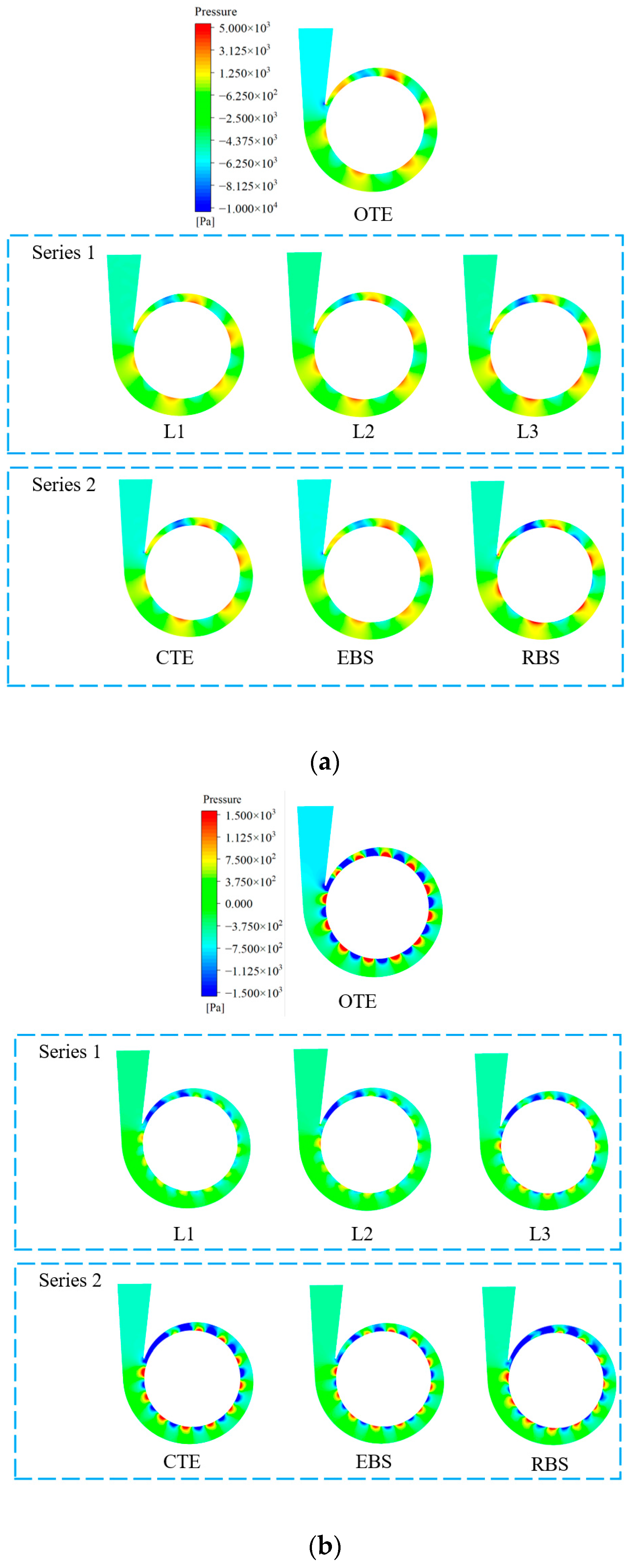
• In Series 1, changing the angles on both sides of the trailing edge primarily affects the pressure on the suction surface. In Series 2, the shape of the trailing edge of a centrifugal pump mainly affects the static pressure on the pressure surface at the rear of the blade. In Series 1, as the angles on both sides of the blade decrease, the pressure fluctuation at the volute tongue decreases; in Series 2, the elliptical edge shape on both sides (EBS) exhibits the smallest pressure fluctuation intensity at the volute tongue, and is 19.6% lower than the original tailing edge (OTE) shape.
• The entropy production is the largest in the volute, and modifying the trailing edge redistributes the proportion of entropy production in different regions. In Series 1 and Series 2, greater entropy generation rates are accompanied by greater pressure pulsations at the pump outlet.
• The energy proportions of the different modes are reflected by a modal analysis of the flow field. The DMD mode corresponding to the BPF and its harmonic frequency is a stable flow structure with a high modal energy. The pressure pulsation is the strongest near the volute tongue. The modal space inhomogeneity (MSI) parameter is defined, which is essentially consistent with the results of the pressure fluctuation analysis. In Series 1, compared with original trailing edge (OTE) shape, the change in the trailing edge angle has little effect on the MSI value of the impeller exit flow field in Mode 1. The MSI value of the impeller exit flow field in Mode 2 decreases compared to the original trailing edge (OTE) shape, and the magnitude of the decrease reduces as the exit angle of the trailing edge increases. In Series 2, the rectangular edge shape on both sides (RBS) exhibits a more uneven distribution compared to the original trailing edge (OTE) shape in Mode 1. The MSI value of the rectangular edge shape on both sides (RBS) is the largest, being 27% greater than that of the original trailing edge (OTE) shape in Mode 1.

6. Innovation and Improvements

The primary innovation of this article lies in analyzing the correlation between the numerical value of modal energy distribution in the volute and the changes in pressure pulsation through the DMD method. Additionally, the study explores the relationship between the impeller outlet modal space inhomogeneity and efficiency under different modes.

However, there are several limitations to the paper. In this paper, only the nominal flow rate of the original trailing edge as analyzed. In fact, the best efficiency points of the different trailing edges were different. In future works, the best efficiency point of the pump for different trailing edges should be found under different flow conditions.

References

1. Yu, T.; Shuai, Z.; Wang, X.; Jian, J.; He, J.; Li, W.; Jiang, C. Research on wake and potential flow effects of rotor–stator interaction in a centrifugal pump with guided vanes. Phys. Fluids 2023, 35, 037107. [Google Scholar] [CrossRef]
2. Zhang, N.; Liu, X.; Gao, B.; Wang, X.; Xia, B. Effects of modifying the blade trailing edge profile on unsteady pressure pulsations and flow structures in a centrifugal pump. Int. J. Heat Fluid Flow 2019, 75, 227–238. [Google Scholar] [CrossRef]
3. Huang, B.; Zeng, G.; Qian, B.; Wu, P.; Shi, P.; Qian, D. Pressure fluctuation reduction of a centrifugal pump by blade trailing edge modification. Processes 2021, 9, 1408. [Google Scholar] [CrossRef]
4. Cui, B.; Li, W.; Zhang, C. Effect of blade trailing edge cutting angle on unstable flow and vibration in a centrifugal pump. J. Fluids Eng. 2020, 142, 101203. [Google Scholar] [CrossRef]
5. Gao, B.; Zhang, N.; Li, Z.; Ni, D.; Yang, M. Influence of the blade trailing edge profile on the performance and unsteady pressure pulsations in a low specific speed centrifugal pump. J. Fluids Eng. 2016, 138, 051106. [Google Scholar] [CrossRef]
6. Wu, D.; Yan, P.; Chen, X.; Wu, P.; Yang, S. Effect of trailing-edge modification of a mixed-flow pump. J. Fluids Eng. 2015, 137, 101205. [Google Scholar] [CrossRef]
7. Zhang, F.; Xiao, R.; Zhu, D.; Liu, W.; Tao, R. Pressure pulsation reduction in the draft tube of pump turbine in turbine mode based on optimization design of runner blade trailing edge profile. J. Energy Storage 2023, 59, 106541. [Google Scholar] [CrossRef]
8. Li, B.; Li, X.; Jia, X.; Chen, F.; Fang, H. The role of blade sinusoidal tubercle trailing edge in a centrifugal pump with low specific speed. Processes 2019, 7, 625. [Google Scholar] [CrossRef]
9. Lin, Y.; Li, X.; Zhu, Z.; Wang, X.; Lin, T.; Cao, H. An energy consumption improvement method for centrifugal pump based on bionic optimization of blade trailing edge. Energy 2022, 246, 123323. [Google Scholar] [CrossRef]
10. Wang, C.; Wang, F.; Zou, Z.; Xiao, R.; Yang, W. Effect of lean mode of blade trailing edge on hydraulic performance for double-suction centrifugal pump. In IOP Conference Series. Earth and Environmental Science; IOP Publishing: Bristol, UK, 2019; p. 032030. [Google Scholar]
11. Denton, J.D. Entropy generation in turbomachinery flows. SAE Trans. 1990, 99, 2251–2263. [Google Scholar]
12. Sun, Q.; Naterer, G.; Fraser, D. Towards integration of turbine blade design and entropy generation minimization. In Proceedings of the 4th AIAA Theoretical Fluid Mechanics Meeting, ON, Ontario Canada, 6–9 June 2005; p. 5321. [Google Scholar]
13. Wang, M.; Li, Z.; Han, G.; Yang, C.; Zhao, S.; Zhang, Y.; Lu, X. Vortex dynamics and entropy generation in separated transitional flow over a compressor blade at various incidence angles. Chin. J. Aeronaut. 2022, 35, 42–52. [Google Scholar] [CrossRef]
14. Huang, P.; Appiah, D.; Chen, K.; Zhang, F.; Cao, P.; Hong, Q. Energy dissipation mechanism of a centrifugal pump with entropy generation theory. AIP. Adv. 2021, 11, 045208. [Google Scholar] [CrossRef]
15. El-Gendi, M.M.; Lee, S.W.; Joh, C.Y.; Lee, G.S.; Son, C.H.; Chung, W.J. Elliptic trailing edge for a turbine blade: Aerodynamic and aerothermal effects. Trans. Jpn. Soc. Aeronaut. Space Sci. 2013, 56, 82–89. [Google Scholar] [CrossRef]
16. Hoseinzade, D.; Lakzian, E.; Dykas, S. Optimization of the trailing edge inclination of wet steam turbine stator blade towards the losses reduction. Exp. Tech. 2023, 47, 269–279. [Google Scholar] [CrossRef]
17. Zhou, C.; Hodson, H.; Himmel, C. The effects of trailing edge thickness on the losses of ultrahigh lift low pressure turbine blades. J. Turbomach. 2014, 136, 081011. [Google Scholar] [CrossRef]
18. Zhang, Q.; Du, J.; Li, Z.; Li, J.; Zhang, H. Entropy generation analysis in a mixed-flow compressor with casing treatment. J. Therm. Sci. 2019, 28, 915–928. [Google Scholar] [CrossRef]
19. Lin, D.; Yuan, X.; Su, X. Local entropy generation in compressible flow through a high pressure turbine with delayed detached eddy simulation. Entropy 2017, 19, 29. [Google Scholar] [CrossRef]
20. Nazeryan, M.; Lakzian, E. Detailed entropy generation analysis of a Wells turbine using the variation of the blade thickness. Energy 2018, 143, 385–405. [Google Scholar] [CrossRef]
21. Qi, B.; Zhang, D.; Geng, L.; Zhao, R.; Van Esch, B.P.M. Numerical and experimental investigations on inflow loss in the energy recovery turbines with back-curved and front-curved impeller based on the entropy generation theory. Energy 2022, 239, 122426. [Google Scholar] [CrossRef]
22. Khan, N.; Shah, Z.; Islam, S.; Khan, I.; Alkanhal, T.; Tlili, I. Entropy generation in MHD mixed convection non-Newtonian second-grade nanoliquid thin film flow through a porous medium with chemical reaction and stratification. Entropy 2019, 21, 139. [Google Scholar] [CrossRef] [PubMed]
23. Hayat, T.; Khan, M.; Qayyum, S.; Khan, M.; Alsaedi, A. Entropy generation for flow of Sisko fluid to rotating disk. J. Mol. Liquids 2018, 264, 375–385. [Google Scholar] [CrossRef]
24. Schmid, P.J.; Sesterhenn, J. Dynamic mode decomposition of experimental data. In Proceedings of the 8th International Symposium on Particle Image Velocimetry, Melbourne, VIC, Australia, 25–28 August 2009. [Google Scholar]
25. Schmid, P.J. Dynamic mode decomposition of numerical and experimental data. J. Fluid Mech. 2010, 656, 5–28. [Google Scholar] [CrossRef]
26. Mariappan, S.; Gardner, A.D.; Richter, K.; Raffel, M. Analysis of Dynamic Stall Using Dynamic Mode Decomposition Technique. AIAA J. 2014, 52, 2427–2439. [Google Scholar] [CrossRef]
27. Callaham, J.; Brunton, S.; Loiseau, J. On the Role of Nonlinear Correlations in Reduced-Order Modelling. J. Fluid Mech. 2022, 938, A1. [Google Scholar] [CrossRef]
28. Yin, G.; Ong, M. Numerical Analysis on Flow around a Wall-Mounted Square Structure Using Dynamic Mode Decomposition. Ocean Eng. 2021, 223, 108647. [Google Scholar] [CrossRef]
29. Zhao, M.; Zhao, Y.; Liu, Z. Dynamic Mode Decomposition Analysis of Flow Characteristics of an Airfoil with Leading Edge Protuberances. Aerospace Sci. Technol. 2020, 98, 105684. [Google Scholar] [CrossRef]
30. Sakai, M.; Sunada, Y.; Imamura, T.; Rinoie, K. Experimental and Numerical Studies on Flow behind a Circular Cylinder Based on POD and DMD. Trans. Jpn. Soc. Aeronaut. Space Sci. 2015, 58, 100–107. [Google Scholar] [CrossRef]
31. Han, Y.; Tan, L. Dynamic mode decomposition and reconstruction of tip leakage vortex in a mixed flow pump as turbine at pump mode. Renew. Energy 2020, 155, 725–734. [Google Scholar] [CrossRef]
32. Liu, M.; Tan, L.; Cao, S. Method of dynamic mode decomposition and reconstruction with application to a three-stage multiphase pump. Energy 2020, 208, 118343. [Google Scholar] [CrossRef]
33. Liu, H.; Sun, J.; Xu, C.; Lu, X.; Sun, Z.; Zheng, D. Numerical Simulation and Dynamic Mode Decomposition Analysis of the Flow Past Wings with Spanwise Waviness. Eng. Appl. Comput. Fluid Mech. 2022, 16, 1849–1865. [Google Scholar] [CrossRef]
34. Li, Y.L.Y.; He, C.; Li, J. Study on Flow Characteristics in Volute of Centrifugal Pump Based on Dynamic Mode Decomposition. Math. Probl. Eng. 2019, 2019, 2567659. [Google Scholar] [CrossRef]
35. Guo, Y.; Gao, L.; Mao, X.; Ma, C.; Ma, G. Dynamic mode decomposition for the tip unsteady flow analysis in a counter-rotating axial compressor. Phys. Fluids 2023, 35, 116106. [Google Scholar] [CrossRef]
36. Li, Q.; Wu, P.; Wu, D. Study on the transient characteristics of pump during the starting process with assisted valve. In Fluids Engineering Division Summer Meeting; American Society of Mechanical Engineers: New York, NY, USA, 2017. [Google Scholar]
37. Otmani, A.; Slimane, N.; Sahrane, S.; Dekhane, A.; Azzouz, S. CFD investigation on three turbulence models for centrifugal pump application. Eurasia Proc. Sci. Technol. Eng. Math. 2022, 21, 202–213. [Google Scholar] [CrossRef]
38. Al-Obaidi, A.R. Effects of Different Turbulence Models on Three-Dimensional Unsteady Cavitating Flows in the Centrifugal Pump and Performance Prediction. Int. J. Nonlinear Sci. Numer. Simul. 2019, 20, 487–509. [Google Scholar] [CrossRef]
39. Li, H.; Chen, Y.; Yang, Y.; Wang, S.; Bai, L.; Zhou, L. CFD simulation of centrifugal pump with different impeller blade trailing edges. J. Mar. Sci. Eng. 2023, 11, 402. [Google Scholar] [CrossRef]
40. Zhang, X.; Jiang, C.; Lv, S.; Wang, X.; Yu, T.; Jian, J.; Shuai, Z.; Li, W. Clocking Effect of Outlet RGVs on Hydrodynamic Characteristics in a Centrifugal Pump with an Inlet Inducer by CFD Method. Eng. Appl. Comput. Fluid Mech. 2021, 15, 222–235. [Google Scholar] [CrossRef]
41. Ni, S.; Zhao, G.; Chen, Y.; Cao, H.; Jiang, C.; Zhou, W.; Shuai, Z. Modulation effect on rotor-stator interaction subjected to fluctuating rotation speed in a centrifugal pump. Eng. Appl. Comput. Fluid Mech. 2023, 17, 2163703. [Google Scholar] [CrossRef]
42. Kock, F.; Herwig, H. Entropy production calculation for turbulent shear flows and their implementation in cfd codes. Int. J. Heat Fluid Flow 2005, 26, 672–680. [Google Scholar] [CrossRef]
43. Liu, C.; Wang, Y.; Yang, Y.; Duan, Z. New omega vortex identification method. Sci. China Phys. Mech. Astron. 2016, 59, 684711. [Google Scholar] [CrossRef]
Figure 1. (a) Components of the pump. (b) Centrifugal pump model.
Processes 12 00508 g001aProcesses 12 00508 g001b
Figure 2. Different trailing edge shapes: (a) original trailing edge (OTE), (b) L1, (c) L2, (d) L3, (e) circular trailing edge (CTE), (f) elliptical edge on both sides (EBS), and (g) rectangular edge on both sides (RBS).
Processes 12 00508 g002
Figure 3. Contour on the original trailing edge shape of the impeller.
Processes 12 00508 g003
Figure 4. Mesh of the fluid domain: (a) boundary layers; (b) impeller.
Processes 12 00508 g004
Figure 5. Grid independence analysis of the original trailing edge shape pump.
Processes 12 00508 g005
Figure 6. Layout of the closed test system.
Processes 12 00508 g006
Figure 7. (a) Dimensionless pump head and (b) pump efficiency under the experimental and simulation conditions.
Processes 12 00508 g007
Figure 8. Static pressure distribution on a single blade with different trailing edges. Series 1: (ac); Series 2: (df).
Processes 12 00508 g008
Figure 9. (a) Streamwise direction in the volute. (b) Impeller outlet velocity triangle.
Processes 12 00508 g009
Figure 10. Radial velocity at the impeller outlet based on different trailing edge types: (a) Series 1 and (b) Series 2.
Processes 12 00508 g010
Figure 11. Time history plots of pressure pulsations at the impeller outlet.
Processes 12 00508 g011
Figure 12. Entropy generation rate (EGR) detection surface.
Processes 12 00508 g012
Figure 13. EGR distribution of the different trailing edges under a nominal flow rate.
Processes 12 00508 g013
Figure 14. Distribution of the vortex nuclei at the different trailing edges at 1.0 Q , where Ω = 0.2, colored by EGR.
Processes 12 00508 g014
Figure 15. Proportion of S P R O ¯ in the different parts.
Processes 12 00508 g015
Figure 16. Total amount of S P R O at the different trailing edges.
Processes 12 00508 g016
Figure 17. Comparison of the different trailing edge heads.
Processes 12 00508 g017
Figure 18. Comparison of the efficiency of the different trailing edges.
Processes 12 00508 g018
Figure 19. Pressure fluctuations at the volute tongue under the designed flow rate: (a) Series 1 and (b) Series 2.
Processes 12 00508 g019aProcesses 12 00508 g019b
Figure 20. Pressure fluctuation intensity in the volute domain: (a) Series 1 and (b) Series 2.
Processes 12 00508 g020
Figure 21. Pressure fluctuation intensity at the volute tongue.
Processes 12 00508 g021
Figure 22. Spectrum of the pressure fluctuation at the volute outlet under nominal flow: (a) Series 1 and (b) Series 2.
Processes 12 00508 g022
Figure 23. Stability analysis of the main frequencies: (a) eigenvalues and (b) growth rates.
Processes 12 00508 g023
Figure 24. Pressure contour of Mode 0.
Processes 12 00508 g024
Figure 25. Energy distribution of DMD modal energy and modal energy proportion.
Processes 12 00508 g025
Figure 26. Evolution of the pressure amplitude at the volute tongue after DMD: (a) Mode 1 of Series 1, (b) Mode 1 of Series 2, (c) Mode 2 of Series 1, and (d) Mode 2 of Series 2.
Processes 12 00508 g026
Figure 27. Pressure contour of DMD: (a) Mode 1 and (b) Mode 2.
Processes 12 00508 g027
Figure 28. Evolution of the pressure amplitude using DMD in the space around the volute: (a) Mode 1 of Series 1, (b) Mode 1 of Series 2, (c) Mode 2 of Series 1, and (d) Mode 2 of Series 2.
Processes 12 00508 g028