
Calculation Method of the Phase Recovery of Gas Cap Reservoir with Bottom Water


1
School of Petroleum Engineering, Yangtze University, Wuhan 430113, China
2
Cooperative Innovation Center of Unconventional Oil and Gas, Yangtze University, Wuhan 430113, China
3
School of Petroleum Engineering, Southwest Petroleum University, Chengdu 610500, China
4
Research Institute of Exploration and Development, Zhongyuan Oilfield Company, China Petrochemical Corporation, Puyang 457000, China
*
Author to whom correspondence should be addressed.
Processes 2024, 12(3), 551; https://doi.org/10.3390/pr12030551
Submission received: 10 January 2024
/
Revised: 6 March 2024
/
Accepted: 9 March 2024
/
Published: 11 March 2024
Abstract
:In gas cap reservoirs underlain by bottom water, the connection between the reservoir and the aquifer leads to an increasing invasion of bottom water as reservoir development progresses. The average formation pressure of the reservoir will change, and the separated phase recovery of the gas cap reservoir with bottom water will be affected by the change in the average formation pressure. The traditional average formation pressure calculation formulas do not consider the water influx, so the accurate calculation of separated recovery cannot be obtained by those calculation methods. The development of gas cap reservoirs with bottom water presents several challenges, including the simultaneous production of oil and gas, undetermined rates of bottom water influx, and uncertain formation pressure and gas-to-oil ratios. These factors contribute to substantial discrepancies between theoretical calculations and actual observations. A more accurate and comprehensive approach is required to address these issues and enable a precise determination of the phase separated recovery in gas cap reservoirs with bottom water. The volume-deficit method is integrated with the Fetkovich quasi-steady state method for water influx. The water-influx prediction is incorporated into the material balance equation, which is further refined by introducing the Fetkovich model to enhance the estimation of the average formation pressure. The average formation pressure, once determined, is utilized in conjunction with the established relationships among this pressure, surface oil production, gas production, and the dissolved gas–oil ratio. Through the application of mass conservation principles, the varying degree of phase recovery, as influenced by fluctuations in the average formation pressure, is calculated. The precision of this refined method has been validated by a comparison with outcomes generated by simulation software. The results reveal a commendable accuracy: an error in the average formation pressure calculation is found to be merely 2.61%, while the errors in recovery degrees for gas cap gas, dissolved gas, and oil-rim oil are recorded at 2.73%, 2.94%, and 1.28%, respectively. These minor discrepancies indicate a good level of consistency and affirm the reliability of this advanced methodology, as demonstrated by passive assessments. This paper provides a method to accurately calculate the phase recovery without some oil- and gas-production data, which provides accurate data support for the actual production evaluation and subsequent development measures.
1. Introduction
The average formation pressure is a critical quantity for the dynamic analysis of oil and gas reservoirs, as well as the determination of the recovery since it serves as an important indicator of the production process of these reservoirs. Accurately determining the average formation pressure, which varies in real time, is very important. Numerous elements influence formation pressure, encompassing a range of geological variables such as sedimentary diversity and diagenetic heterogeneity observed within reservoirs. These variables include variations in bedding planes, disparities in porosity, intricate pore structures, mineralogical composition differences, and the heterogeneous physical properties of rocks. These disparities can lead to differences in pressure and permeability across the varied pore and fracture networks, significantly impacting the productivity and flow characteristics of the formation fluids. Consequently, these factors play a crucial role in shaping the distribution and evolution of formation pressure, as well as its distribution and evolution process [1]. There are many methods for analyzing and calculating the average formation pressure; measurement and calculation methods are commonly used to determine the average formation pressure [2,3,4]. Many scholars have proposed average formation pressure methods for the measured method, including Matthews et al.’s MBH method for reservoirs, the point pressure calculation method for gas wells, etc. Most of these methods calculate the average formation pressure of oil reservoirs and gas reservoirs by pressure-recovery test wells [5,6,7,8,9]. However, the actual measurement method requires a long time to shut down the well for formation pressure recovery. The test cycle is long, and as a result, the average formation pressure cannot be tracked in real time. It will also cause different degrees of economic losses to the normal production of the oil and gas reservoir [10,11]. The calculation method can determine the pressure in real time, and the commonly used basic methods are the material balance equation and the flowing-material balance method; the former requires gas wells to conduct the shut-in pressure recovery, it is difficult to obtain the critical point-formation pressure of gas wells in the proposed steady state with the latter, and there are certain limitations in both methods [12,13,14]. Therefore, it is very important to calculate the average formation pressure with no well shut-ins by using the production dynamic information, which is relatively easy to obtain, and then provide data support for the subsequent calculation of the fractional phase recovery of the reservoir.
Addressing the unique characteristics of these methodologies, the material balance equation, integrated with dynamic production data, has been utilized by researchers in recent years for estimating the average formation pressure. Varied investigations into different formation pressure-evaluation methods, tailored to specific oil and gas reservoirs, have been conducted.
In 2013, the reverse condensate process, influenced by porous media adsorption and capillary forces, was investigated by Wu et al. The water-vapor content of condensate gas under various pressures was tested, and a material balance equation for water-drive condensate gas reservoirs, incorporating the effects of porous media adsorption, capillary forces, and water vapor, was established based on material balance principles. This equation was then solved iteratively to determine the formation pressure at any particular time during production. During the development of condensate gas reservoirs, condensate oil begins to precipitate once the formation pressure falls below the bubble-point pressure. This precipitation is intensified by porous media adsorption and capillary pressure. Concurrently, the continuous evaporation of formation water increases water-vapor content within the condensate gas, thereby influencing the variation in formation pressure. Should local formation pressure persistently decline while the content of condensate and steam concurrently rises, the disparity between various calculated results will also expand. Notably, the formation pressure estimated through the specially established material balance equation, which considers the impacts of adsorption, capillary pressure, and steam, is more accurate, exhibiting a smaller comparative error with actual pressure measurements [15].
In 2014, Zhang et al. examined the joint development dynamics of the gas cap and oil rim in condensate gas reservoirs featuring an oil rim. It was identified that a continual decrease in the formation pressure triggered reverse condensation phenomena within the gas cap while simultaneously leading to the release of dissolved gas from the oil rim. This release was associated with several changes, including the evaporation of primary water, the expansion of rock fluids, and edge- and bottom-water encroachment. In light of these considerations, a prediction method for formation pressure, specifically for condensate gas reservoirs with an oil rim, rooted in the mass conservation principle of hydrocarbon fluids, was devised. The formation pressure estimated through this approach strongly agreed with actual shut-in pressure measurements, confirming its reliability. During modes of depleted production, it was observed that increased production rates from both the gas cap and oil rim could accelerate the drop in the formation pressure. Additionally, it was noted that when the pore volume of the gas cap surpasses that of the oil rim, an elevation in the gas-production rate more readily exacerbates the fall in the formation pressure. Consequently, it is recommended to maintain the gas-production rate at moderate levels to avert the premature exhaustion of formation energy [16].
Yang et al. developed a methodology that deduces the connection between bottom-hole flow pressure and formation pressure under specific assumptions: a closed boundary, no edge or bottom water, uniform reservoir thickness, and extraction solely based on elastic energy, which disregards pore volume and bound-water compressibility. This was achieved by integrating natural gas’s high-pressure physical property variations with pressure, the principle of material balance, and the gas reservoir’s seepage mechanism. The approach led to the formulation of a partial differential equation linking formation pressure with production data, allowing for the calculation of the average formation pressure directly from production figures without necessitating well shut-ins. The technique, applied under varying conditions of total gas extraction, stable production durations, and cumulative production times, demonstrated an error margin of less than 2% compared to numerical simulation outcomes, showcasing high precision. Nonetheless, due to its idealized foundational assumptions, this model is limited to specific reservoir conditions and is inapplicable to other types of reservoir-production scenarios [11].
Jiang et al. adopted the empirical formula of Standing–Katz fitted by the Beggs–Robinson–Wilson (BRW) state equation to determine the deviation coefficient (Z value) based on the pressure and temperature in a constant volume gas reservoir. They plotted the relationship curve between the bottom-hole flowing pressure (pwf) divided by Z and the cumulative gas production (GP), then determined the slope of the linear segment of this curve. Utilizing this slope alongside the initial formation pressure, they formulated the material balance equation specific to a closed, constant-volume gas reservoir. By applying this equation, they calculated the current formation pressure using the derived apparent formation pressure and cumulative production data. The methodology’s validity was confirmed by comparing the calculated values against actual measurements, revealing a marginal error of 3.8%, which attests to the reliability and feasibility of this approach for estimating formation pressures [17].
Tao et al. enhanced the principle of material balance by incorporating the dynamic shifts in high-pressure physical properties of rocks and fluids with varying formation pressures. They developed a real-time applicable formula for formation-pressure calculations that accommodates changes in both the rock-pore volume and the oil–water volume, effectively covering both the elastic-production and water-injection development stages. Following precise experimental determinations of the high-pressure physical parameters of rocks and fluids, the team could implement accurate formation-pressure calculations. The material balance method yielded an average formation pressure for the M reservoir at 40.5 MPa, displaying a minimal discrepancy of only 0.5 MPa from well test-interpretation results. Furthermore, the error margin between reductions in rock pore volume and fluid volume was noted to be 2%, underlining the reliability of the used physical parameters. This innovative material balance approach offers a fresh perspective for real-time and precise formation-pressure evaluations in closed or weak-edge and bottom-water reservoirs using production-performance data. However, this method exhibits limitations: it yields less accurate results for oil and gas reservoirs with strong edge and bottom-water drives, unknown volume, or those operating under dissolved gas-drive and saturation-pressure conditions [18].
Zhang et al. developed a material balance equation for gas reservoirs, which excludes the impact of edge- and bottom-water encroachment but includes the effects of rock-pore volume contraction and bound-water expansion. They established a mathematical model for gas percolation, deriving solutions for both constant and variable production scenarios in terms of pseudo pressure. In conditions where constant production reaches a quasi-steady state and variable production enters the stage of the boundary-controlled flow, the team formulated approximate conditions for quasi-steady state pressure and material balance, respectively. By integrating these two formulations, they provided a methodology for an iterative computation of the average formation pressure. The method demonstrated an average error of 8.6% when compared to actual measured formation pressures, thus satisfying the requirements for engineering applications. Nonetheless, this approach does not account for the influx of edge and bottom water and is, therefore, not applicable to gas reservoirs influenced by active aquifers [19].
Yin et al. embarked on a detailed study of single wells, segregating the immediate vicinity into two distinct zones: the supply boundary and the supply area. They employed the principle of mass conservation to devise a material balance equation that encapsulates various factors such as the well injection-production ratio, production rate, fluid volume coefficient, overall compressibility coefficient, porosity, and average formation pressure. Following the establishment of quasi-steady state conditions, radial-flow mathematical models for both the supply boundary and supply area were developed and integrated into the material balance equation, leading to distinct formation-pressure formulas for each zone. Comparing the formation pressures calculated through this methodology against those measured empirically showed a discrepancy of only 2.7%, underscoring the method’s practical reliability and applicability in real-world scenarios [20].
Zhang et al. developed a productivity model for closed, elastic-driven gas reservoirs, starting from the material balance equation. This model, framed in terms of pseudo pressure, activates once the pressure wave contacts the boundary. It accounts for the variations in the deviation coefficient and bottom-hole flow pressure relative to the average formation pressure, and it delineates the relationship between these pressures when the formation pressure is above or below a reference pressure. By integrating the established average formation pressure and bottom-hole flow-pressure formulas into the material balance framework, the model facilitates an iterative calculation of the average formation pressure using production data. Validation of the method revealed that both the gas-production rate and the recovery significantly influence the model’s outcomes. An application example demonstrated that the method’s calculated results have a small relative error compared to those from pressure build-up well tests, with an error margin of 4.85%, which is acceptable within the parameters of engineering calculations [3].
Wu Nan et al. introduced a material balance-inversion method that leverages minimal pressure monitoring data, combined with mathematical inversion techniques, to assess the formation pressure in tight sandstone gas reservoirs. Initially, the method utilizes production data from gas wells under a quasi-stable flow state to fit a Blasingame chart, facilitating the calculation of the dynamic reserves. Subsequently, the dynamic reserves and a single pressure-measurement datum are inverted to formulate the material balance equation, into which the cumulative gas production is input to evaluate the formation pressure. This method was applied to a tight sandstone gas well in the Daning–Jixian block, resulting in the computation of formation pressure. The discrepancy between the calculated-average formation pressure and the actual measured formation pressure was 1.76%. The findings indicate that (1) the material balance-inversion method, requiring only a single-pressure measurement point, effectively evaluates changes in the formation pressure of gas wells; (2) the initial formation pressure in gas wells can exhibit significant variations, with individual wells demonstrating complex pressure behaviors and multiple pressure systems; (3) discrepancies among pressure systems correlate strongly with pronounced reservoir heterogeneity [21].
Table 1 shows the average formation pressure, measured formation pressure, and corresponding errors calculated by various methods in the investigated literature:
Phase recovery is the ratio of the cumulative production of each phase to the geological reserves of each phase in an oil and gas field over a period of time. It is a crucial comprehensive index for measuring the effectiveness and level of oilfield development. The commonly used methods for calculating the recovery include empirical formulae and analytical methods. In 1965,Eaton B A and Jacoby R H proposed an empirical formula for the recovery of condensate with a condensate content of 73–400 g/m3 and the use of depletion type extraction by studying the basic parameters of 27 condensate reservoirs in the U.S.A. [22]. In 2005, C.S. Kabir, for the cyclic injection of gas to extract the condensate reservoirs, introduced the reinjection ratio, which includes the injection and extraction of wells and gas by using the “C” method. The study also introduced parameters such as the reinjection ratio, injection and extraction well spacing, average permeability, and condensate content, which is the proposed empirical formula for condensate recovery [23]. In 2020, Xiong Yu et al. proposed an empirical formula for the condensate recovery by introducing parameters such as the reinjection ratio, injection and extraction well spacing, average permeability, and condensate content in the study of the Tarim–Yaha cyclic gas injection and condensate extraction reservoir [24]. Most of these methods are based on the empirical formula method, which is often derived based on oilfield production dynamic data, and whether the calculation result is reasonable and the matching degree between empirical formula and reservoir type and has the limitation of application. In the analytical method, in 2004, under the production mode of gas-injection development, Che Wenlong et al. used the material balance method to convert the produced condensate into gas, plus the produced dry gas, and deducted the injected dry-gas value as the cumulative gas production, but there was a big deviation between the calculation results of this method and the actual situation [25]. In 2014, Zhang Angang et al. established the formula of calculating the amount of change in the amount of hydrocarbon fluids in the formation equal to the amount of cumulative hydrocarbon fluids through the principle of conservation of hydrocarbon materials. The formula can calculate the cumulative yield of each phase to calculate the recovery of each phase, but it does not consider the unknown situation of the water influx [16].
It is a common method to establish the material balance equation to calculate the average formation pressure, which has good accuracy in calculating the average formation pressure of closed- or weak-water reservoirs but performs poorly in calculating comprehensive reservoirs with strong side-bottom water. The commonly used formulaic method of phase recovery depends on the match between the empirical formula and the reservoir type, and the analytical method has factors that are not considered or cannot calculate the phase recovery that varies with the pressure in real time. To address these problems, based on the previous research, it is proposed to combine the predicted water influx amount and material balance method to establish an expression formula about the average formation pressure. After obtaining the average formation pressure, the phase recovery was calculated using the law of conservation of mass after obtaining the average formation pressure.
2. Methods
2.1. Analysis of the Oil and Gas Reservoirs
Gas-cap reservoirs with bottom water are a special class of oil reservoirs. They have both oil and gas fields, with gas zones in the upper part and oil zones in the lower part, and they are externally connected to a body of water. These fluids are in a state of kinetic-, thermodynamic-, and fluid-phase equilibrium during reservoir formation [26]. As a special kind of oil reservoir, gas-cap bottom-water reservoirs have been explored and practiced for many years, and different extraction effects have been obtained in different oil fields. In the development process of this kind of reservoir, the relative stability of the oil-water interface, as well as the gas-oil interface, should be considered to avoid unfavourable factors such as the sudden advance of bottom water and the cone of bottom water. Considering the change of water influx and ignoring the influence of water vapour in the water phase, the average formation pressure is determined by applying the Fetkovich model to the material balance equation. After obtaining the average formation pressure, it is proposed to calculate the phase recovery with the change of the average formation pressure by adopting the law of conservation of mass according to the surface oil and gas production and the dissolved gas–oil ratio.
During its development, the pressure of formation decreases, and the original equilibrium state of the reservoir is destroyed. The distribution of phase changes before and after development is shown in Figure 1: When the pressure is greater than the bubble-point pressure, there is no liquid in the gas cap, the bottom water advances, the water vapour of the water phase enters more into the gas cap, the bottom water intrudes into the oil zone, and the main driving energy of gas reservoir is gas-elastic performance [15,16]. When the formation pressure is less than the bubble-point pressure, the subsurface fluid produces phase changes, and the dissolved gas in the crude oil precipitates, the water vapour in the aqueous phase further escapes, the sideprime water further intrudes, and the elastic expansion of the rock and bound water occurs, and so on, in a series of phase transformations and energy exchanges [15,27,28,29,30,31].
2.2. Average Formation Pressure
With gas cap reservoir and bottom-water pressure drop, gas, water, the oil rim, and so on, will expand accordingly. The extracted gas, including the gas from the cap and the dissolved part, was precipitated in the oil rim. After the pressure drops to PMPA, the volume of crude oil includes the volume of produced oil, the reduction of pore volume, and the expansion of bound water volume., the formula is:
The remaining volume at the gas cap is the difference between the original free and dissolved gas, and the extracted gas and remaining dissolved gas, considering the expansion of the gas from the cap. Then, the formula is:
The volume change of water body is the invasive water body minus the mining water body. Then, the added water body is calculated as:
After a certain volume of crude oil and gas is extracted from an oil reservoir, the formation pressure decreases, and the water at the bottom of the margin will intrude into the reservoir. According to the material balance relationship, the combined volume of oil and gas extracted should be equal to the increased volume of water, so the formula is obtained:
Assuming , as well as , further collation of the above equation is obtained:
In the above equation, Np represents the cumulative oil production in units of m3. Bo represents the oil-volume factor in units of m3/m3. Rp represents the production gas–oil ratio in units of m3/m3. Rs represents the dissolved gas–oil ratio in units of m3/m3. Bg represents the gas-volume factor in units of m3/m3. Wp represents the cumulative water production in units of m3. Bw represents the water-volume factor in units of m3/m3. We represents cumulative water influx in units of m3. N represents the petroleum reserves in units of m3. Boi represents the original oil-volume factor in units of m3/m3. Rsi represents the original dissolved gas–oil ratio in units of m3/m3. m represents the ratio of the volume of gas-bearing zone to the volume of oil-bearing zone. Bgi represents the original gas-volume factor in units of m3/m3. Swc represents irreducible water saturation. cw represents the compression factor of formation water in units of MPa−1. cp represents the compression factor of rock-pore volume in units of MPa−1. pi represents the original formation pressure in units of MPa. p represents the formation pressure in units of MPa. Bt represents the crude-oil two-phase volume factor in units of m3/m3. Bti represents the original crude-oil two-phase volume factor in units of m3/m3.
This material balance equation is obtained by Ralpgh. J. Schilthuis equation, Li Chuanliang’s integrated drive-reservoir material balance relationship combined with the study of reservoir block-derivation algorithm [32].
In general, the reservoir-production history and PVT characteristic parameters are known, while the water influx We is an unknown value, and the water influx at each pressure measurement point is calculated using the volume-deficit method.
Let the variable X denote the formation energy loss:
The deficit volume of a gas-cap reservoir without considering water influx is:
The deficit volume of a gas-cap reservoir considering water influx is:
By associating Equations (5)–(8), the water-influx volume is calculated as the difference between the deficit volume of the reservoir considering water influx and not considering water influx, which is calculated:
The application of the volume-deficit method can only calculate the water influx at the pressure-measurement point, but the water influx at the non-pressure measurement point cannot be obtained. In order to address this problem, the whole average formation pressure that changes with the development of the oilfield is calculated by invoking Fetkovich’s proposed steady-state water-influx method in conjunction with the volume deficit method.
Using Fetkovich’s proposed steady-state water-influx method [33], the water-influx volume We was calculated:
where Wei represents the maximum water influx:
Water influx coefficient B:
In the above equations, Vw represents the volume of water body in units of 104 m3. J represents the water influx index in units of m3/d/MPa. t represents the time in units of day.
By constantly adjusting the maximum water-influx amount Wei and water-influx index J, the water-influx amount calculated by Fetkovich’s proposed steady-state water influx method at the pressure measurement point is the closest to the water influx amount calculated by the volumetric-deficit method. The water-influx amount We calculated in Fetkovich’s proposed steady-state water-influx method was brought into the material balance equation of the gas-cap reservoir and simplified to obtain:
The average formation pressure at any particular time can be calculated using the Newton iteration method, which is:
In the above equations, ct represents the total compressibility in units of MPa−1.
The average formation pressure obtained with the process of reservoir development can be used to conduct the calculation of the recovery of the sub-phase to provide data support.
The material balance equation and Formulas (7)–(9) for a gas-cap reservoir with water influx are derived by modifying Li Chuanliang’s comprehensive drive-reservoir material-balance relationship. This relationship calculates the entire reservoir as a whole and often does not consider the direction of fluid flow, making it a zero-dimensional model of reservoir fluid flow [32]. Newton’s iterative method is quoted from numerical analysis books [34].
Since this block is a reservoir with the presence of gas cap, during the production process, when the pressure drops below the saturation pressure, the dissolved gas is released, resulting in the cumulative production of gas Gp, which includes both gas-cap gas and dissolved gas. In solving the recovery of split-phase, using the phase-balance theory, material-balance theory, and the principle of equivalence of fugacity [33,35,36,37,38,39], based on the relationship between the dissolved gas–oil ratio and the average formation pressure, the daily gas production is categorized, and the daily oil-rim oil production, daily dissolved gas production, and daily gas-cap gas production are calculated, and the cumulative production of each split-phase is obtained by superposition, of which the phase recovery is calculated.
2.3. Calculation of Phase Recovery
The daily gas production qg consists of dissolved gas qg1 and gas-cap gas qg2. The daily oil production qo consists of oil-rim oil qo1. The gas- and oil-production equations can be calculated separately by associating them:
The formulas for the daily oil-rim oil production qo1, the daily dissolved-gas production qg1, and the daily gas-cap gas production qg2, respectively, are as follows:
Total dissolved gas reserves Gs:
The phase recovery of oil-rim oil, dissolved gas, and gas-cap gas can be obtained by comparing the cumulative production of each component with the total reserves:
In the above equations, qg represents the gas production in units of m3. qg1 represents the dissolved gas production in units of m3. qg2 represents the cap-gas production in units of m3. qo represents the oil production in units of m3. qo1 represents the oil-rim oil production in units of m3. Rs represents the dissolved gas–oil ratio in units of m3/m3. Gs represents the total dissolved gas reserves in units of m3. G2 represents the total cap-gas reserves in units of m3. ro1 represents the oil recovery from the oil rim. rg1 represents the dissolved gas recovery. rg2 represents the gas recovery from the gas cap.
2.4. Method Flowchart
The complete flowchart of the calculation method is shown in Figure 2.
3. Results
3.1. Model Establishment
Based on the actual production data of a mining plate in the CQ oilfield, using digital analog software tNavigator, a component model is used to simulate a bottom-water water-driven gas-cap reservoir production well, considering the expansion of bound water, rocks, and gas cap. The model is 325 m × 1300 m × 28 m, the crude-oil geological reserve is 2.33 × 10⁵ m3, the gas reserve is 7.62 × 10⁷ m3, the initial formation pressure is 19.7 MPa, the formation temperature is 389.3 K, the water-phase volume coefficient is 1, the crude-oil volume coefficient is 1.5, and the ratio of gas-cap volume-to-reservoir volume is 0.7. The original porosity is 0.2, the original gas saturation of the gas cap zone is 70%, and the radial permeability is 220 mD. The pressure of this gas-cap reservoir will be gradually reduced in the process of extraction, and the set extraction time is 6.78 years. According to the actual production data of the oilfield, the mechanism model of the gas-cap reservoir with bottom water is constructed, as shown in Figure 3, to simulate the whole development process.
The pressure p, crude-oil volume coefficient Bo, gas-deviation coefficient Z value, and dissolved gas–oil ratio Rs obtained by PVT, as well as experimental measurements, are shown in Table 2, and the regression relationships between pressure p and crude-oil volume coefficient Bo, gas-deviation coefficient Z value, and dissolved gas–oil ratio Rs are shown in Equations (23)–(25).
3.2. Calculation Steps and Results
Oil- and gas-production data from the data-body model were incorporated into Equations (6)–(9) for the volumetric-deficit method and Equations (10)–(12) for Fetkovich’s steady-state water-influx method. The water-influx Index J was iteratively adjusted to align the water-influx volumes derived from both methods. The outcomes of these calculations are depicted in Figure 4, where the estimated error in water influx is identified as 5.9%. Production dynamics data, along with the amounts and coefficients of water influx, were applied to Equations (14) and (15) using Newton’s iterative method to calculate average formation pressure. The efficacy of this approach was corroborated by comparing the average formation-pressure results from the method introduced by Cai Jianqin with those obtained from this study. Figure 5 illustrates the comparison between the average formation pressures determined by the current method, those derived from Cai’s approach, and those calculated by the tNavigator numerical simulation software (tNavigator v21.1-1615-g08bcf3ac6cb).
The actual output of gas is split into two parts, which are the gas from the cap and dissolved gas; the output oil is oil-rim oil. According to the law of mass conservation, using the daily gas–oil production, the daily oil-rim oil production qo1, the daily dissolved gas production qg1, and the daily gas-cap gas production qg2 were calculated by combining Equation (16), Equation (17), and Equation (18), respectively, and the dissolved gas reserve Gs1 was calculated by utilizing Equation (19), and the daily production of sub-phases was totaled and calculated with the original reserves of each sub-phase by utilizing Equations (20)–(22) to obtain the extraction levels of gas-cap gas, oil-rim oil, and dissolved gas at different pressures, respectively. The recovery levels of gas cap, oil rim, and dissolved gas at different pressures were obtained. Simulation calculations were conducted by using tNavigator simulation software to simulate the mechanism model of gas-cap and bottom-water reservoirs, and some results of the calculations are shown in Table 3:
The accuracy of the proposed method is verified by comparing it with the results of the phase-recovery degree calculated by tNavigator numerical simulation software, which is used as a calculation control group for comparative judgment. The phase-recovery degree calculated by numerical modeling software, comparison method introduced and the phase-recovery degree calculated based on the average formation-pressure method, is displayed below. Group A represents the results of the phase-recovery degree calculated by numerical modeling software, Group B represents the degree of split-phase extraction calculated based on the average formation pressure approach, and Group C represents the further calculation of the phase-separation extraction degree based on the introduced method and the data provided in the article. The comparison curves are shown in Figure 6.
4. Discussion
The average formation pressure is the basis for evaluating the productivity and analyzing the potential of oil and gas reservoirs. The average formation-pressure calculation of oil and gas reservoirs varies with the types of oil and gas reservoirs, geological parameters, fluid properties, development methods, and whether the means of production are complete. The gas-cap reservoir with bottom water discussed in this paper is a kind of reservoir with different storage forms. In the process of exploitation, the extraction of crude oil and natural gas will reduce the formation pressure and lead to the invasion of bottom water, which makes the variation law of formation pressure different from that of conventional oil and gas reservoirs, resulting in errors in the calculation of the phase recovery. Therefore, a new method is proposed to calculate the accurate average formation pressure by calculating the water influx so as to accurately calculate the phase recovery.
4.1. Average Formation Pressure
As the reservoir is developed, the pressure in the formation drops rapidly at first, and then the rate of decline is slower. This is because as oil and gas are produced, the rapid pressure drop leads to bottom-water influx, which rapidly fills the volume vacated by the produced oil and gas, and the pressure drop gradually decreases. The real-time water-influx volume can be calculated by this method, and the real-time average formation pressure can be calculated by combining it with the material balance equation. The maximum error between the calculated average formation pressure and the value calculated by tNavigator numerical simulation is 2.61%, which is a small error. The error between the average formation pressure calculated by the introduced method and the average formation pressure calculated by digital simulation is 2.7%, which is close to the error of the method introduced in this paper. It shows that the method introduced in this paper is feasible.
4.2. Phase Recovery
The comparison curve is shown in Figure 4 and analyzed in combination with Table 2. During the exploitation of gas-cap gas, with the decrease of average formation pressure, the water influx increases rapidly, and the recovery curves of gas-cap gas, dissolved gas, and oil-rim oil rise rapidly. Among them, the recovery curve of gas-cap gas rises fastest, indicating that the natural gas produced at this stage is mainly gas-cap gas. In the comparison curve, the recovery of gas cap calculated by the method proposed in this paper is slightly smaller, and the correlation curve of dissolved gas is intertwined, which is caused by the small error in the calculation of average formation pressure. At the beginning of the middle stage, a large amount of bottom water has invaded, and the rising rate of water influx has decreased compared with the previous stage, which gradually reduces the decline of pressure, and the recovery of gas cap gas tends to be gentle. The dissolved gas and oil-rim oil still maintain a large increase with the decline of average formation pressure in the production process. At this time, the calculated value in the comparison curve by the method proposed in this paper is slightly larger. The average errors of the recovery of gas-cap gas, dissolved gas, and oil-rim oil calculated by the two methods are 2.73%, 2.94%, and 1.28%, respectively. Comparing the phase recovery calculated by the quoted method, combined with the existing data with the phase recovery calculated by the mathematical model, the recovery errors of gas cap gas, dissolved gas, and oil rim oil are 1.4%, 3.9%, and 7.6%, respectively. The overall error is small. Compared with the method mentioned in this paper, the calculation error is smaller, which shows that the method proposed in this paper is feasible.
5. Conclusions
In this paper, a methodology is introduced that integrates water-influx prediction with the material balance equation for gas-cap reservoirs containing bottom water, establishing a functional equation for average formation pressure. The Newton iteration method is employed to resolve this equation, facilitating the determination of the average formation pressure at any point during the production lifecycle of oil and gas reservoirs. Utilizing the established relationship between average formation pressure and production-performance data, the phase recovery, as influenced by changes in average formation pressure, is deduced through the application of mass conservation principles. The average relative errors between the phase recovery, as determined by this method and those calculated by digital simulation software, are found to be 2.73%, 2.94%, and 1.28%, respectively. This approach enables the continuous calculation of the phase recovery throughout the extraction process, providing essential data support for real-time production assessment.
Our future work will involve applying field data from varied geological reservoir settings to validate the proposed method, aiming to minimize calculation errors and enhance the robustness and applicability of the model. Additionally, efforts will be made to adapt the methodology for use in heterogeneous and multiphase fluid reservoirs to extend its practical utility. Moreover, future research will explore the incorporation of machine-learning techniques to refine water-influx predictions, aiming to reduce computational complexity and enhance efficiency.
Author Contributions
Writing—original draft preparation, M.L.; writing—review and editing, Y.Z.; methodology, L.Y. and M.L.; software, M.L. and X.G.; visualization, B.J. and M.Z. All authors have read and agreed to the published version of the manuscript.
Funding
This research was funded by National Natural Science Foundation of China, grant number 52004032.
Data Availability Statement
Data are contained within the article.
Conflicts of Interest
Author Long Yang was employed by the company Research Institute of Exploration and Development, Zhongyuan Oilfield Company, SINOPEC. The remaining authors declare that the research was conducted in the absence of any commercial or financial relationships that could be construed as a potential conflict of interest.
Nomenclatures
| Np | Cumulative oil production (m3) |
| Bo | Oil-volume factor (m3/m3) |
| Rp | Production gas–oil ratio (m3/m3) |
| Rs | Dissolved gas–oil ratio(m3/m3) |
| Bg | Gas-volume factor (m3/m3) |
| Wp | Cumulative water production (m3) |
| Bw | Water-volume factor (m3/m3) |
| We | Volume of cumulative intrusion of reservoir water (m3) |
| N | Petroleum resources (m3) |
| Boi | Original oil volume factor (m3/m3) |
| Rsi | Original dissolved gas–oil ratio (m3/m3) |
| m | Ratio of the volume of gas-bearing zone to the volume of oil-bearing zone |
| Bgi | Original gas-volume factor (m3/m3) |
| Swc | Irreducible water saturation (f) |
| cw | Compression factor of formation water (MPa−1) |
| cp | Compression factor of rock-pore volume (MPa−1) |
| pi | Original formation pressure (MPa) |
| p | Formation pressure (MPa) |
| Bt | Crude-oil two-phase volume factor (m3/m3) |
| Bti | Original crude-oil two-phase volume factor (m3/m3) |
| Vw | Volume of water body (104 m3) |
| J | Water-influx index (m3/d/MPa) |
| t | Time (d) |
| ct | Total compressibility (MPa−1) |
| qg | Gas production (m3) |
| qg1 | Dissolved gas production (m3) |
| qg2 | Top gas production (m3) |
| qo | Oil production (m3) |
| qo1 | Oil-rim oil production (m3) |
| Gs | Total dissolved gas reserves (m3) |
| G2 | Total top gas reserves (m3) |
| Z | Compressibility factor (dless) |
| ro1 | Oil recovery from the oil rim |
| rg1 | Dissolved gas recovery |
| rg2 | Gas recovery from the gas cap |
References
- Jamil, M.; Siddiqui, N.A.; Rahman, A.H.B.A.; Ibrahim, N.A.; Ismail, M.S.B.; Ahmed, N.; Usman, M.; Gul, Z.; Imran, Q.S. Facies Heterogeneity and Lobe Facies Multiscale Analysis of Deep-Marine Sand-Shale Complexity in the West Crocker Formation of Sabah Basin, NW Borneo. Appl. Sci. 2021, 11, 5513. [Google Scholar] [CrossRef]
- Wang, Y.; Zhou, X.; Yin, C.; Shu, P.; Cao, B.; Zhu, Y. Gas accumulation conditions and key exploration & development technologies in Xushen gas field. Shiyou Xuebao/Acta Pet. Sin. 2019, 40, 866–886. [Google Scholar] [CrossRef]
- Zhang, L.; Wang, Y.; Ni, J.; Qiao, X.; Xin, C.; Zhang, T.; Kang, Y.; Shi, J.; Wu, K. A new method for tracking and calculating average formation pressure of gas reservoirs. Shiyou Xuebao/Acta Pet. Sin. 2021, 42, 492–499+522. [Google Scholar] [CrossRef]
- Wenpeng, B.; Shiqing, C.; Yang, W.; Dingning, C.; Xinyang, G.; Qiao, G. A transient production prediction method for tight condensate gas wells with multiphase flow. Pet. Explor. Dev. 2023, 51, 154–160. [Google Scholar] [CrossRef]
- Miller, C.C.; Dyes, A.B.; Hutchinson, C.A., Jr. The Estimation of Permeability and Reservoir Pressure from Bottom Hole Pressure Build-Up Characteristics. J. Pet. Technol. 1950, 2, 91–104. [Google Scholar] [CrossRef]
- Matthews, C.S.; Brons, F.; Hazebroek, P. A Method for Determination of Average Pressure in a Bounded Reservoir. Trans. AIME 1954, 201, 182–191. [Google Scholar] [CrossRef]
- Brons, F.; Miller, W.C. A Simple Method for Correcting Spot Pressure Readings. J. Pet. Technol. 1961, 13, 803–805. [Google Scholar] [CrossRef]
- Dietz, D.N. Determination of Average Reservoir Pressure from Build-Up Surveys. J. Pet. Technol. 1965, 17, 955–959. [Google Scholar] [CrossRef]
- Bingyu, J. Some understandings on the development trend in research of oil and gas reservoir engineering methods. Acta Pet. Sin. 2020, 41, 1774–1778. [Google Scholar] [CrossRef]
- Muskat, M. Use of Data Oil the Build-Up of Bottom-Hole Pressures. Trans. AIME 1937, 123, 44–48. [Google Scholar] [CrossRef]
- Yongqing, Y. Calculation of average reservoir pressure by using modified flowing material balance. Fault-Block Oil Gas Field 2015, 22, 747–751. [Google Scholar]
- Mattar, L.; McNeil, R. The “Flowing” Gas Material Balance. J. Can. Pet. Technol. 1998, 37, PETSOC-98-02-06. [Google Scholar] [CrossRef]
- Mattar, L.; Anderson, D.; Stotts, G. Dynamic Material Balance-Oil-or Gas-in-Place without Shut-Ins. J. Can. Pet. Technol. 2006, 45, PETSOC-06-11-TN. [Google Scholar] [CrossRef]
- Gonzalez, F.E.; Ilk, D.; Blasingame, T.A. A Quadratic Cumulative Production Model for the Material Balance of an Abnormally Pressured Gas Reservoir. In Proceedings of the SPE Western Regional and Pacific Section AAPG Joint Meeting, Bakersfield, CA, USA, 29 March–2 April 2008. [Google Scholar] [CrossRef]
- Wu, K.-L.; Li, X.-F.; Fan, J.; Li, Y.-J.; Wu, L. An approach to calculate water influx and aquifer region of abnormally high pressure condensate gas reservoir. Zhongguo Kuangye Daxue Xuebao/J. China Univ. Min. Technol. 2013, 42, 105–111. [Google Scholar] [CrossRef]
- Zhang, A.; Fan, Z.; Song, H.; Zhang, H. Reservoir pressure prediction of gas condensate reservoir with oil rim. Zhongguo Shiyou Daxue Xuebao (Ziran Kexue Ban)/J. China Univ. Pet. (Ed. Nat. Sci.) 2014, 38, 124–129. [Google Scholar] [CrossRef]
- Yanfang, J. Feasibility Analysis of Calculating Formation Pressure with the Production Data in Daniudi Gas Field. 2016, 18, 30–33. J. Chongqing Univ. Sci. Technol. 2016, 18, 30–33. [Google Scholar] [CrossRef]
- Yongfu, T.; Rui, X.; Liang, Q.; Jun, Z.; Guohui, F.; Huaqin, Z. Evaluation of formation pressure in M reservoir of Yaerxia Oilfield by material balance method. Oil Gas Well Test. 2019, 28, 72–78. [Google Scholar] [CrossRef]
- Zhang, L.; Guo, C.; Jiang, H.; Cao, G.; Chen, P. Gas in place determination by material balance-quasipressure approximation condition method. Shiyou Xuebao/Acta Pet. Sin. 2019, 40, 337–349. [Google Scholar] [CrossRef]
- Hongjun, Y.; Gang, W.; Cuiqiao, X.; Jing, F.; Fakcharoenphol, P. Average Formation Pressure Calculation for the Composite Oil Reservoir with Multi-Well System. Spec. Oil Gas Reserv. 2019, 26, 76–80. [Google Scholar] [CrossRef]
- Nan, W.; Shi, S.; Shiqi, Z.; Haoyang, Z.; Hongya, W.; Jiangnan, T. Formation pressure calculation of tight sandstone gas reservoir based on material balance inversion method. Coal Geol. Explor. 2022, 50, 115–121. [Google Scholar] [CrossRef]
- Eaton, B.A.; Jacoby, R.H. A New Depletion-Performance Correlation for Gas-Condensate Reservoir Fluids. J. Pet. Technol. 1965, 17, 852–856. [Google Scholar] [CrossRef]
- Kabir, C.S.; Badru, O.; Eme, V.; Carr, B.S. Assessing Producibility of a Region’s Gas/Condensate Reservoirs. In Proceedings of the SPE Annual Technical Conference and Exhibition, Dallas, TX, USA, 9–12 October 2005. [Google Scholar] [CrossRef]
- Yu, X. Theory and Application of Dynamic Analysis of Cyclic Gas Injection in Condensate Reservoirs. Ph.D. Thesis, Southwest Petroleum University, Chengdu, China, 2020. [Google Scholar] [CrossRef]
- Chen, W.; Wu, D.; Wu, N.; Zhang, M.; Wang, M.; Wu, Z. The research of performance monitoring technique in yaha condensate gas reservoir of tarim basin. Nat. Gas Geosci. 2004, 15, 553–558. [Google Scholar]
- Jiao, H.; Sun, W.; Sun, Y. Development practices and procedures of gas cap reservoirs in China. Petrochem. Ind. Technol. 2020, 27, 96+99. [Google Scholar] [CrossRef]
- Chen, Y. Application and derivation of material balance equation for abnormally pressured gas reservoirs. Acta Pet. Sin. 1983, 4, 45–53. [Google Scholar] [CrossRef]
- Begland, T.F.; Whitehead, W.R. Depletion Performance of Volumetric High-Pressured Gas Reservoirs. SPE Reserv. Eng. 1989, 4, 279–282. [Google Scholar] [CrossRef]
- Fetkovich, M.J.; Reese, D.E.; Whitson, C.H. Application of a General Material Balance for High-Pressure Gas Reservoirs. SPE J. 1998, 3, 3–13. [Google Scholar] [CrossRef]
- Jing, X.; Xingli, X.; Guang, J.; Kai, L. Derivation and application of material balance equation for over-pressured gas reservoir with aquifer. Acta Pet. Sin. 2007, 28, 96–99. [Google Scholar] [CrossRef]
- Liu, D.; Liu, Z.; Tian, Z. A modified material balance equation for abnormal-pressure gas reservoirs with aquifer. Acta Pet. Sin. 2011, 32, 474–478. [Google Scholar] [CrossRef]
- Chuanliang, L. Principles of Reservoir Engineering, 3rd ed.; Petroleum Industry Press: Beijing, China, 2017; pp. 150–188. [Google Scholar]
- Zhao, L.; Bian, D.; Fan, Z.; Song, H.; Li, J.; Zhao, X. Oil property changes during the waterflooding for reservoirs with condensate gas cap. Pet. Explor. Dev. 2011, 38, 74–78. [Google Scholar] [CrossRef]
- Li, Q.; Wang, N.; Yi, D. Numerical Analysis, 5th ed.; Huazhong University of Science & Technology Press: Wuhan, China, 2018; pp. 149–153. [Google Scholar]
- Mehra, R.K.; Heidemann, R.A.; Aziz, K. Computation of Multiphase Equilibrium for Compositional Simulation. Soc. Pet. Eng. J. 1982, 22, 61–68. [Google Scholar] [CrossRef]
- Wang, N.; Chen, Z.; Zhu, M.; Wang, Y.; Zhang, Y. Dynamic reserve calculation of single well in condensate gas reservoirs based on a principle of mass conservation. Nat. Gas Geosci. 2018, 29, 424–428. [Google Scholar] [CrossRef]
- Pereira, V.J.; Regueira, V.B.; Costa, G.M.N.; Vieira de Melo, S.A.B. Modeling the Saturation Pressure of Systems Containing Crude Oils and CO2 Using the SRK Equation of State. J. Chem. Eng. Data 2019, 64, 2134–2142. [Google Scholar] [CrossRef]
- Gorgonio, F.-C.; Mario, A.V.-C. Reservoir performance analysis through the material balance equation: An integrated review based on field examples. J. Pet. Sci. Eng. 2022, 208, 109377. [Google Scholar] [CrossRef]
- Jianqin, C.; Tao, L.; Xiaojian, W.; Jinling, Z.; Yong, T.; Jiazheng, Q.; Jiehong, T. A New Method to Predict Average Reservoir Pressure for Oil Reservoir Subject to Edge or Bottom Water Drive Considering Time-Varying Water Influx. Drill. Prod. Technol. 2023, 46, 89–93. [Google Scholar] [CrossRef]
Figure 1.
Schematic of fluid distribution before and after development of gas-cap bottom-water reservoirs.
Figure 1.
Schematic of fluid distribution before and after development of gas-cap bottom-water reservoirs.
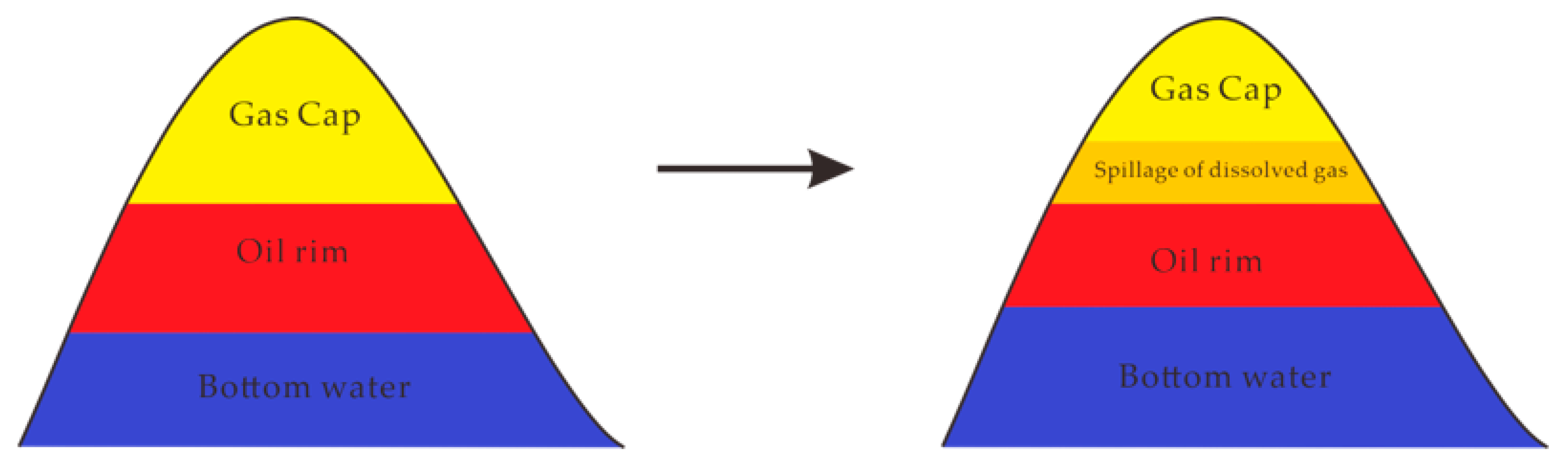
Figure 2.
Calculation flowchart.

Figure 3.
Mechanism model of gas-cap reservoir with bottom water.

Figure 4.
Comparison of calculation results of water encroachment.

Figure 5.
Comparison of results of average formation pressure calculated by three different methods.
Figure 5.
Comparison of results of average formation pressure calculated by three different methods.

Figure 6.
Comparison of the calculation results of the recovery of gas in gas cap, dissolved gas, and oil-rim oil phase. (a) Comparison of calculation results of gas recovery of gas cap; (b) comparison of calculation results of dissolved gas recovery; (c) comparison of calculation results of oil recovery of oil rim.


Table 1.
Various methods and errors for calculating average formation pressure.
| Title of the Article | Calculated Average Formation Pressure | Measured Formation Pressure | Error/% |
|---|---|---|---|
| Calculation of average reservoir pressure by using modified flowing material balance | 16.90 | 16.71 | 1.14 |
| Feasibility analysis of calculating formation pressure with the production data in Daniudi gas field | 15.80 | 15.20 | 3.8 |
| Evaluation of formation pressure in M reservoir of Yaerxia oilfield by material balance method | 30.6 | 31.1 | 1.6 |
| Gas in place determination by material balance-quasipressure approximation condition method | 44.28 | 40.74 | 8.6 |
| Average formation-pressure calculation for the composite oil reservoir with multi-well system | 11.250 | 11.565 | 2.7 |
| A new method for tracking and calculating average formation pressure of gas reservoirs | 13.241 | 13.916 | 4.85 |
| Formation pressure calculation of tight sandstone gas reservoir based on material balance-inversion method | 4.54 | 4.46 | 1.76 |
Table 2.
Pressure and fluid parameters.
| P (MPa) | Rs (m3/m3) | Bo | Z |
|---|---|---|---|
| 18.00 | 111.1 | 1.4494 | 0.9367 |
| 17.00 | 105.2 | 1.4399 | 0.9332 |
| 15.00 | 93.0 | 1.4064 | 0.9341 |
| 10.00 | 60.8 | 1.3526 | 0.9450 |
| 5 | 30.4 | 1.2525 | 0.9688 |
Table 3.
Table of numerical modeling results for gas-cap reservoirs with bottom water.
| P | Rs | Bo | Bg | Bt | Z | qo | qg (104) | qo | Gp (105) |
|---|---|---|---|---|---|---|---|---|---|
| 19.150 | 117.884 | 1.459 | 0.008 | 1.490 | 0.953 | 19.401 | 17.778 | 734.116 | 42.344 |
| 17.859 | 110.259 | 1.448 | 0.008 | 1.585 | 0.948 | 8.150 | 4.703 | 2021.839 | 160.231 |
| 16.765 | 103.752 | 1.437 | 0.009 | 1.693 | 0.945 | 4.132 | 1.573 | 3591.385 | 231.510 |
| 16.532 | 102.362 | 1.435 | 0.009 | 1.719 | 0.944 | 4.093 | 1.220 | 3952.333 | 243.710 |
| 16.165 | 100.169 | 1.431 | 0.009 | 1.762 | 0.943 | 3.478 | 0.799 | 4602.825 | 261.279 |
| 15.899 | 98.573 | 1.428 | 0.009 | 1.795 | 0.943 | 3.554 | 0.523 | 5236.246 | 272.736 |
| 15.688 | 97.309 | 1.426 | 0.009 | 1.822 | 0.942 | 3.521 | 0.340 | 5884.221 | 281.016 |
| 15.543 | 96.439 | 1.424 | 0.009 | 1.841 | 0.942 | 3.496 | 0.223 | 6495.854 | 285.925 |
| 15.426 | 95.732 | 1.423 | 0.009 | 1.857 | 0.942 | 3.214 | 0.101 | 7117.166 | 289.023 |
| 15.351 | 95.283 | 1.422 | 0.009 | 1.868 | 0.942 | 3.306 | 0.097 | 7625.719 | 290.508 |
| 15.286 | 94.888 | 1.421 | 0.010 | 1.877 | 0.942 | 3.627 | 0.044 | 8248.482 | 291.765 |
| 15.232 | 94.563 | 1.420 | 0.010 | 1.884 | 0.941 | 3.026 | 0.033 | 8825.444 | 292.426 |
| 15.183 | 94.271 | 1.420 | 0.010 | 1.891 | 0.941 | 2.742 | 0.028 | 9363.980 | 293.012 |
| 15.147 | 94.057 | 1.419 | 0.010 | 1.896 | 0.941 | 2.423 | 0.024 | 9810.439 | 293.474 |
Disclaimer/Publisher’s Note: The statements, opinions and data contained in all publications are solely those of the individual author(s) and contributor(s) and not of MDPI and/or the editor(s). MDPI and/or the editor(s) disclaim responsibility for any injury to people or property resulting from any ideas, methods, instructions or products referred to in the content. |
© 2024 by the authors. Licensee MDPI, Basel, Switzerland. This article is an open access article distributed under the terms and conditions of the Creative Commons Attribution (CC BY) license (https://creativecommons.org/licenses/by/4.0/).
Share and Cite
MDPI and ACS Style
Li, M.; Zhang, Y.; Zhang, M.; Ju, B.; Yang, L.; Guo, X. Calculation Method of the Phase Recovery of Gas Cap Reservoir with Bottom Water. Processes 2024, 12, 551. https://doi.org/10.3390/pr12030551
AMA Style
Li M, Zhang Y, Zhang M, Ju B, Yang L, Guo X. Calculation Method of the Phase Recovery of Gas Cap Reservoir with Bottom Water. Processes. 2024; 12(3):551. https://doi.org/10.3390/pr12030551
Chicago/Turabian StyleLi, Mingzhe, Yizhong Zhang, Maolin Zhang, Bin Ju, Long Yang, and Xu Guo. 2024. "Calculation Method of the Phase Recovery of Gas Cap Reservoir with Bottom Water" Processes 12, no. 3: 551. https://doi.org/10.3390/pr12030551
Note that from the first issue of 2016, this journal uses article numbers instead of page numbers. See further details here.