Abstract
Polymerization products are indispensable for our daily life, and the relevant modeling process plays a vital role in improving product quality. However, the model identification of the related process is a difficult point in industry due multivariate, nonlinear and time-varying characteristics. As for the conventional offline subspace identification methods, the identification accuracy may be not satisfying. To handle such a problem, an enhanced on-line recursive subspace identification method is presented on the basis of principal component analysis and sliding window (RSIMPCA-SW) in this paper to obtain the state space model for polymerization. In the proposed on-line subspace identification approach, the initial L-factor is acquired by the LQ decomposition of the sampled historical data, firstly, and then it is updated recursively through the bona fide method after the new data have been handled by the sliding window rule. Subsequently, principal component analysis (PCA) is introduced to calculate the extended observation matrix, and finally the on-line model parameters are extracted. Compared with the traditional subspace schemes, smaller computation complexity and higher identification precision are anticipated in the proposed method. A case study on the modeling of the ethylene polymerization verifies the effectiveness of the developed approach, in which the related statistical indexes of the obtained identification model are better.
1. Introduction
Polymerization refers to the process of converting low molecular weight monomers into high molecular weight polymers, and it is quite common in many industries [1]. There are two kinds of polymerization: addition polymerization and condensation polymerization. For addition polymerization, the unsaturated bonds in monomers (typically carbon–carbon double bonds) are opened and reacted with reactive groups in other monomer molecules, which forms polymer chains. Condensation polymerization is a process whereby small molecular units within monomers (typically dimers or oligomers) are linked together to form larger polymer molecules. These two types of polymerization reactions play a crucial role in the preparation of polymer materials, and the choice between them depends on the structure, properties and applications of the desired materials. Addition polymerization is usually employed for the synthesis of linear polymers, while condensation polymerization is more suitable for producing branched or crosslinked polymers.
During the past few decades, polymer manufacturing technology has made great progress, with the development of dynamic principles, process mathematical models and so on [2]. It is worth mentioning that relevant modeling is one of the significant points for polymerization, due to the fact that it is of great significance for improving the related industrial production efficiency and product quality [3]. As for polymerization, finding the corresponding modeling is not an easy task because of complex reaction mechanisms, uncertain kinetics processes, etc. [4]. Many scholars contributed to the development of the modeling for polymerization. Early mathematical models were built on the basis of first principles, with researchers focusing on reaction kinetics, thermodynamics, mass transfer and particle science. In [5], polymerization was modeled from the perspectives of polymerization kinetics (micro-scale), system thermodynamics (meso-scale) and reactor performance (macro-scale). The Sanchez–Lacombe equation of state model was utilized to simulate the solubility of industrial alkane penetrants in polyethylene, and the analysis of the results showed that the model could provide an accurate prediction of density in olefin polymerization reactors and further guide the production of linear low-density polyethylene in [6]. Zhang et al. [7] derived a polymer thermal reaction kinetic model in the form of an integral, and two undetermined functions were used to compensate for the changes in the reaction rate in the model, and two correction methods were given simultaneously, which made the kinetic model more applicable and effective. In [8], a multi-scale model of the radical polymerization process was effectively built. The employment of the finite element method solved the difficulty of calculating the cost and accuracy of the Fokker–Planck Equation, which can predict the change in particle size distribution on the mesoscale. The above models, established from first principles, can be utilized as substitutes for some polymerization processes after being validated by experimental data. However, the application of these models in practice may be difficult because of inconvenient and expensive maintenance costs, and these mechanism models are often set up under various assumptions, which lead to inconsistency with the actual process [9].
With the development of computer technology and intelligent algorithms, many vital system identification methods have been put forward for modeling polymerization. In order to solve the constraint of the traditional mechanism model for the polymer extrusion process, a system of fuzzy rules was introduced into the extrusion model to fit the sensitive parameters in [10]. Meanwhile, the system was combined with a genetic algorithm to optimize the model structure, and the relevant simulation verified the good adaptability of the built model. In [11], fuzzy logic was applied to the modeling of a discontinuous polymerization reactor to solve the problem of the mechanism model being unable to track the reactor system with transient behavior effectively, and the obtained nonlinear model could effectively predict the change in the average molecular weight of lactic acid and nylon-6 in the pilot scale polymerization experiments. A method based on an expectation maximization algorithm was utilized to intelligently identify batch polymerization reactor process models by Liu et al. [12]. The developed method was mainly concerned with the unknown inputs of the process system, and it was divided into two steps to calculate the model state and the analytic solution of the inputs.
As an important branch of system identification, the subspace method combines linear algebra, statistics and system theory, and it is aimed at establishing the appropriate state space model for processes [13,14]. Comparing with first-principles modeling and other system identification approaches, the subspace method, which adopts algebraic tools such as QR decomposition and singular value decomposition (SVD), possesses the merits of faster computation, better robustness and so on [15]. On the basis of the obtained state space model, the subsequent advanced control strategies can improve the corresponding key indexes in the process further [16]. And many researchers have focused on the study of off-line subspace identification methods and put forward significant results. In order to achieve the effective identification of linear time-invariant systems, a class of output error methods were developed in [17]. Van et al. [18] derived the subspace state system identification algorithm for mixed deterministic stochastic systems. A subspace method in which the bias can be eliminated was developed, and high identification precision was acquired for industries with colored noises in [19]. In order to realize multivariate predictive control in a continuous polymerization reactor of methyl methacrylate, Song et al. [20] developed a subspace algorithm to recognize the Wiener model of the process and then designed a data-based predictive controller. In [21], the state space model based on the subspace identification method was applied to historical process data and nonlinear ultrasonic data to predict the quality, and the results were verified in the experimental data of polyethylene rotary forming process.
However, the identification performance of the off-line subspace method will be reduced for the time-varying process, which promotes the development of the on-line subspace approaches. And there are also many vital related viewpoints. In order to reduce the computation complexity of the on-line identification method, many researchers focused on the selection of approximate methods to solve the updating problem of SVD. In [22], a propagator method which was commonly utilized in array signal processing was introduced to track the subspace of an observable matrix. Meanwhile, many other researchers designed subspace identification methods through updating QR decomposition or SVD directly. The first-order perturbation theory was employed to implement the recursive form of SVD by Shang et al. [23] and the application of the designed recursive canonical variable analysis method in a continuous stirred tank reactor system for polymerization validated the adaptability of this approach to time-varying processes. In order to realize the high-precision identification of time-varying systems, the Heisenberg QR decomposition and eigenvalue decomposition were united to extract the subspace matrix effectively by Wu et al. [24] Meanwhile, the forgetting factor was also introduced in the developed scheme.
It is a fact that there are various complex characteristics in polymerization and inevitable uncertainties in the related production, which presents a big challenge for the relevant accurate modeling process. As for these on-line subspace methods mentioned above, there is still room for the improvement of the recursive computation speed and the identification performance. In order to acquire the desired model for polymerization, it is essential to build an on-line model identification approach which provides faster recursive speed and improved identification precision. To achieve this study objective, an enhanced on-line recursive subspace identification method on the basis of PCA and sliding window is investigated in this paper. By employing PCA, the estimation accuracy of the extended observable subspace is improved, then the enhanced model identification precision is expected. Meanwhile, the utilization of LQ decomposition and the bona fide method simplify the related calculation steps, and thus a faster recursive speed is also anticipated. To validate the effectiveness of the proposed recursive subspace identification method, a case study on the identification experiment of the dynamic model for polyethylene process is demonstrated.
2. Traditional Offline Subspace Identification Method
2.1. Matrix Definition
For simplicity, the following state space model is introduced for polymerization.
where and are the input and output vectors of the process at time instant , respectively. is the state vector, and and denote the corresponding zero-mean noise vectors. , , and are the relevant parameter matrices of the state space model.
We assume that the length of past horizon is , the length of the future horizon is , and the length of the dataset used for model identification is . We can define the past output stack vector and the future output stack vector as
On this basis, then the above stack vectors can be stacked into the following past and future output Hankel matrices, and their columns are defined as , .
Note that the definitions of the input Hankel matrices , and the noise Hankel matrices , , , are similar to the above formulas and omitted here.
The following input–output Hankel equation is then obtained by the iterative computation of the state space model in Equation (1).
where , are the extended observation matrix and the state sequence with the following definitions.
The remaining two Toeplitz matrices , in Equation (6), are then defined as
2.2. Double-Orthogonal-Projection-Based Subspace Identification Method (2ORT-SIM) [19]
In order to simplify the derivation process, here the noise term in Equation (6) is defined as , and then Equation (6) can be converted into the following form.
To obtain the parameter matrices and , the extended observation matrix needs to be computed, firstly, and then the two required parameter matrices can be extracted from it. Taking the orthogonal projection of Equation (11) onto the orthogonal complement of , the relevant effects on the dataset can be eliminated.
where denotes the projection operator, and is the orthogonal complementary space of the corresponding matrix. By adopting , Equation (12) can be rewritten as
In order to eliminate the effect of in Equation (13), another orthogonal projection needs to be performed. And the following equation is obtained by projecting Equation (13) onto the past input .
If the model input is a persistent excitation, then the following condition is satisfied.
Here, the proof of Equation (15) can be found in reference [19] and the relevant contents are omitted here for brevity. Then, Equation (14) can be transformed into
By taking an SVD for the left-hand side of Equation (16), the following formula is acquired.
The extended observation matrix is estimated as
and then the parameter matrices and are extracted as
where , , . denotes the pseudo-inverse of the matrix.
As for the identification of parameter matrices and , they can be obtained by introducing and to both sides of Equation (11). And the following equation is obtained by utilizing and .
Similarly, will be tenable if model inputs are persistent excitations. That is, the noise in Equation (20) will be eliminated accordingly. For the convenience of subsequent calculations, the remaining items in Equation (20) are defined as follows.
where the corresponding matrix dimensions are and .
Then, the parameter matrices and can be obtained by solving the linear combination in Equation (22) through least squares.
3. Proposed On-Line Subspace Identification Method
Here, the state space model of the polymerization in Equation (1) is also considered, and the relevant equations before Equation (14) can be obtained easily by referring to Section 2.
In order to improve the corresponding identification precision for the polymerization in the presence of various uncertainties in practice and to obtain a smaller computation complexity for the on-line subspace algorithms, here, the recursive technique, which is the integration of LQ decomposition with the bona fide method, is employed to update the model parameters in real time.
The initial L-factor at time instant needs to be obtained, firstly, and the second orthogonal projection performed for Equation (14) is replaced by the following LQ decomposition, in which .
where the variables and in parentheses denote the starting modeling moment and current modeling moment, respectively.
Then, the left-hand side of Equation (14) is equivalent to
Define , and the following formula for the initial L-factor can be constructed by employing the property of .
Then, the bona fide method is utilized to obtain a recursive update expression for .
When the input–output data pairs at time instant are collected, the following equation can be obtained by adding the new dataset to the left-hand side of Equation (23).
The formulas as follows are satisfied according to the LQ decomposition shown in Equation (23).
On the basis of Equation (27), the following equations can be acquired.
Combining Equations (27) and (28) with Equation (26), and redefining the relevant block matrices as
the relationship of reveals that holds, and the recursive updating equations for the L-factor from time instant to time instant can be gained according to .
In order to construct the form of , the following equation is obtained by uniting Equations (30)–(32).
where
In order to improve the estimation precision of the extended observation matrix, PCA, which has a good performance in data feature extraction, is introduced after the L-factor at time instant has been acquired. And the left singular vector can be obtained by carrying out the following PCA on the left-hand side of Equation (33).
where , are the load matrix and score matrix, respectively. Subscripts and denote the main subspace and residual subspace.
When the residual load matrix is acquired by estimation, then the extended observation matrix at time instant can be obtained by the following formula.
Finally, the model parameters at time instant can be gained by referring to Equations (19)–(22).
Remark 1.
Note that the size of the data matrix is fixed in the bona fide method, and the related operation is performed by sliding the data window, and thus the computation complexity of the proposed subspace method is reduced greatly.
Remark 2.
The choice of model order plays a crucial role for the final modeling results. There are two main methods for model order estimation in most subspace methods. One is determined by checking the intervals in the singular value profile of the Hankel matrix, which is called the singular value method [25], and another is determined by the spectrum of the AIC criterion [26]. However, the optimal order of the model may not be obtained because of various unavoidable noises. An effective method for estimating the model order is given for this polyethylene reaction process in this paper. Here, an optional range of the system order is assumed, firstly, and then the errors between the model and the actual value for different orders are calculated. Finally, the order with smaller errors and acceptable computation complexity will be selected as the optimal order.
In order to enhance the readability of the paper, the related detailed steps are summarized as follows for the proposed subspace strategy (Algorithm 1).
| Algorithm 1. Steps for the Proposed RSIMPCA-SW |
| (1) Initialize inputs of the algorithm at time instant , including past horizon , future horizon , number of samples , input dataset , output dataset . |
| (2) Iterative computation of Equation (1) to construct the input–output Hankel formula in Equation (11). |
| (3) For the first orthogonal projection, construct Equation (13) by projecting onto the orthogonal complement of . |
| (4) Perform the LQ decomposition of Equation (23) instead of the second orthogonal projection, and construct for the initial L-factor at time instant . |
| (5) Add the new data at time instant to the last column of the original data matrix to construct Equation (26). |
| (6) Recursive update of L-factor by bona fide method according to Equations (30)–(34). |
| (7) Perform PCA on the L-factor at time instant according to Equation (35). |
| (8) Calculate the extended observation matrix by referring to Equation (36). |
| (9) Extract the model parameters according to Equations (37) and (38). |
| (10) Slide the data window to remove the first column of the data matrix in Equation (26) and return to step 5. |
4. Simulation
4.1. Polyethylene Process Flow Description
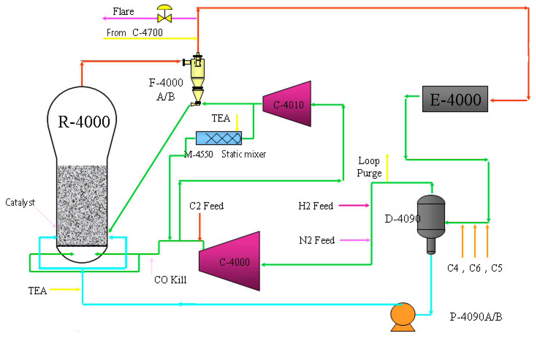
The process described in this section runs on a full-density polyethylene plant, which adopts typical Unipol low pressure gas phase fluidized bed polymerization technology. Here, ethylene is used as the main monomer and butene-1 or hexene-1 is utilized as the co-monomer, with a content range of 1.2–3 wt%. In addition, hydrogen and isopentane are employed as the molecular weight regulator and the condensation inducer, respectively. Note that the operation is carried out in the condensation mode, and it should be guaranteed that the dew point of the circulating gas is above 45 degrees Celsius. During polymerization, the condensate content in the circulating gas is kept at about 10 wt% to improve the reaction efficiency. The products are linear low-density polyethylene and partial medium- and high-density polyethylene particle resin, and the relevant density and melt index ranges are 0.915–0.965 g/cm3 and 0.3–6 g/10 min. This process is mainly divided into the raw material refining system and polymerization system. In terms of the comprehensive product quality and the production cost, this technological process is still the current mainstream technology for polyethylene production. Figure 1 shows the detailed flow chart of the polyethylene process.

Figure 1.
Gas phase fluidized bed polyethylene process flow.
The polymerization system mainly consists of the reactor (R-4000), cooler (E-4000) and compressor (C-4000). The raw materials and catalysts are sent to the fluidized bed reactor continuously from the refining system of polymerization to produce polyethylene resin, and the storage tank (D-4090) stores the intermediate products temporarily. The gas phase materials are circulated under the action of a centrifugal circulating gas compressor and a water-cooled circulating gas cooler incessantly. Circulating gases improve the fluidized bed’s back-mixing ability and carry the reaction material to the reaction zone. At the same time, the circulating gases also take away the heat generated by the exothermic reaction. As for the reactor, it has two discharge systems which operate alternately in general, but can also be operated separately. Each discharge system consists of a product disposal tank and a product ejection tank. The discharge system starts automatically when the reactor bed reaches a predetermined level, and the powder products are dropped continuously from the disposal tank to the ejection tank, and then the power products are transported to the product degassing bin of the degassing system directly. Here, a termination system is set up for the polymerization system, and the polymerization will be stopped partially or completely when the reversible catalyst poison is injected into the reactor. Note that removing the poison from the bed will reactivate the catalyst, and the reaction can be restarted quickly.
4.2. Data Acquisition and Preprocessing
It is not an easy task to choose the appropriate variables for the effective modeling of complex processes. Meanwhile, many variables may not be measured because of the limitations of the relevant measuring sensors. Moreover, variables in the processes are commonly coupled due to the fact that there are multiple sub-reaction processes. All these factors affect the corresponding precision of the process modeling greatly.
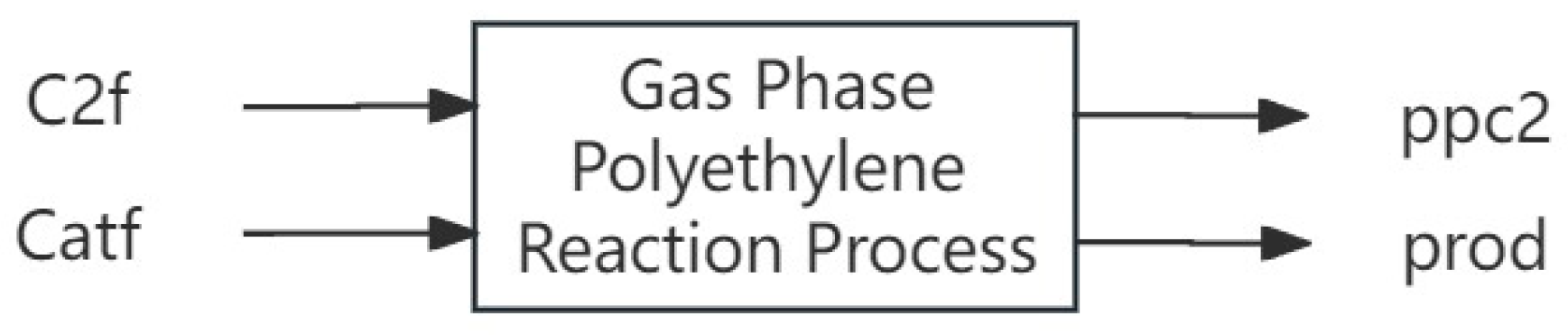
In this section, four typical variables are selected for model identification. Among these, ethylene flow rate (C2f (kg/h)) and catalyst feed amount (Catf (kg/h)) are chosen as inputs, and ethylene partial pressure (ppc2 (ppm)) and polyethylene production (prod (kg/h)) are selected as outputs. Their relationships are shown in Figure 2.
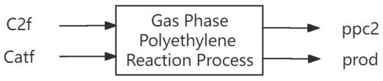
Figure 2.
Variables for subspace identification.
Here, 2000 sets of real sample data collected from a full-density polyethylene plant of a chemical company in 33.3 h (sampling frequency is 60 s) were selected for the simulation. In order to illustrate the effectiveness and generalization ability of the proposed on-line algorithm preferably, a little more data are required for validation, and the ratio of 3:2 was chosen for splitting the 2000 sample data. On the basis of this ratio, the first 1200 samples of the dataset were classified as the identification set, and the remaining 800 samples were chosen as the validation set in the model identification. Since the difference of scale between data is too large, the normalization preprocessing method is utilized, which takes the following form.
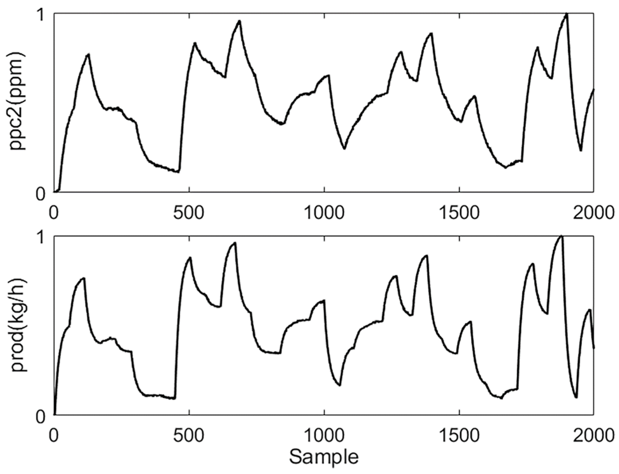
where and denote the data before and after the normalization. are the minimum and maximum values of the corresponding attributes in data. is the relevant lower limit of the magnitude after normalization, and is the related upper limit. The preprocessed data of the process for modeling are shown in Figure 3 and Figure 4.
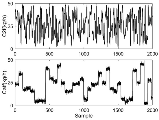
Figure 3.
Preprocessed process input data.
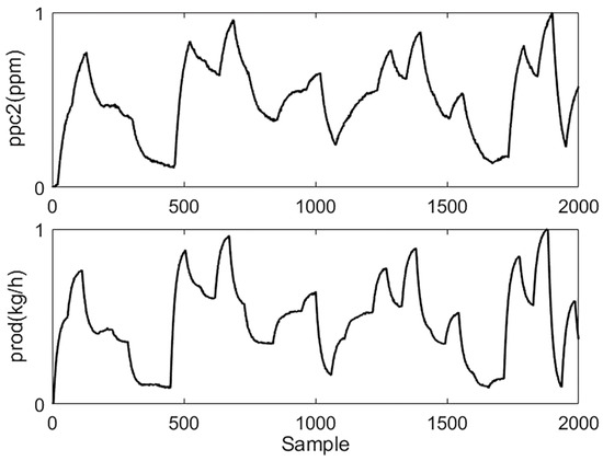
Figure 4.
Preprocessed process output data.
4.3. Model Order Estimation
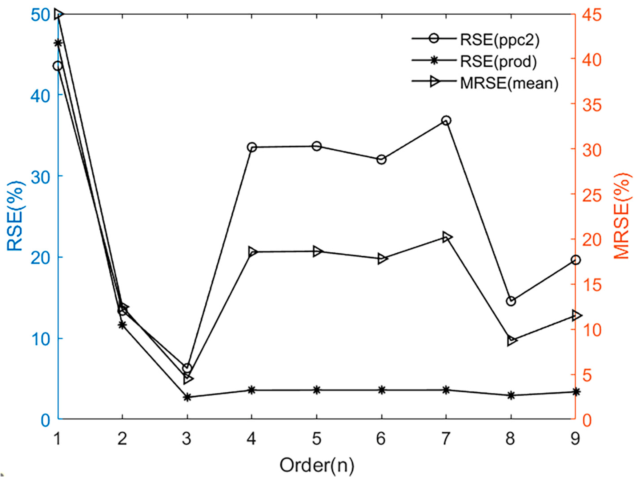
As is mentioned in Remark 2, the first 200 sets of the total sampled dataset are utilized for the model order estimation here, and the relevant error spectrum is shown in Figure 5.
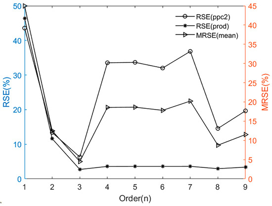
Figure 5.
Error spectrum for different orders.
Here, the theoretical range of the optimal model order is chosen between [1,9] in this section. The circle scatters indicate the distribution of relative squared error (RSE) for ppc2 at each order, and the asterisk scatters indicate the distribution of RSE for prod. The right triangular scatters indicate the average of the two outputs, i.e., the mean relative squared error (MRSE). It can be easily seen that the model possesses the minimum value of MRSE at . Here, the MRSE values for some higher orders may be also acceptable; however, modeling the polymerization with a lower order can reduce the relevant complexity for the subsequent controller design, and thus the optimal model order is selected as 3 here.
4.4. Identification Results and Validation Analysis
The initial input parameters of the proposed algorithm are set as follows: the length of the past horizon is , the length of the future horizon is , and the number of total samples is . In order to verify the effectiveness of the proposed algorithm further, several existing off-line subspace identification algorithms (MOESP [17], N4SID [18], 2ORT-SIM [19]) and the on-line subspace identification algorithm (OSIMPCA-E [24]) are introduced as the comparison. Here, the 1200 sets of sample data in the identification set are used for the relevant training.
Then, the 800 sets of sample data in the validation set are utilized to test the prediction accuracy of these built models in this section, and the RSE, mean absolute error (MAE) and variance accounted for (VAF) are calculated to evaluate the corresponding model accuracy.
The calculation methods of RSE and MAE are shown in Equations (40) and (41), and their values range from 0 to 1. When their values are close to 0, a high matching degree between the prediction model and the actual process will be obtained. The VAF is calculated as shown in Equation (42); note that an ideal identification precision is expected when its value is near 1.
where denotes the number of samples in the validation set. is the sampling serial number, and and represent the actual value and the model predicted value of the th data, respectively.
Note that fixed identified models are used for these off-line methods, and recursive update models are adopted for on-line approaches. And the related statistical results of these algorithms are given in Table 1.

Table 1.
Statistical results of different algorithms.
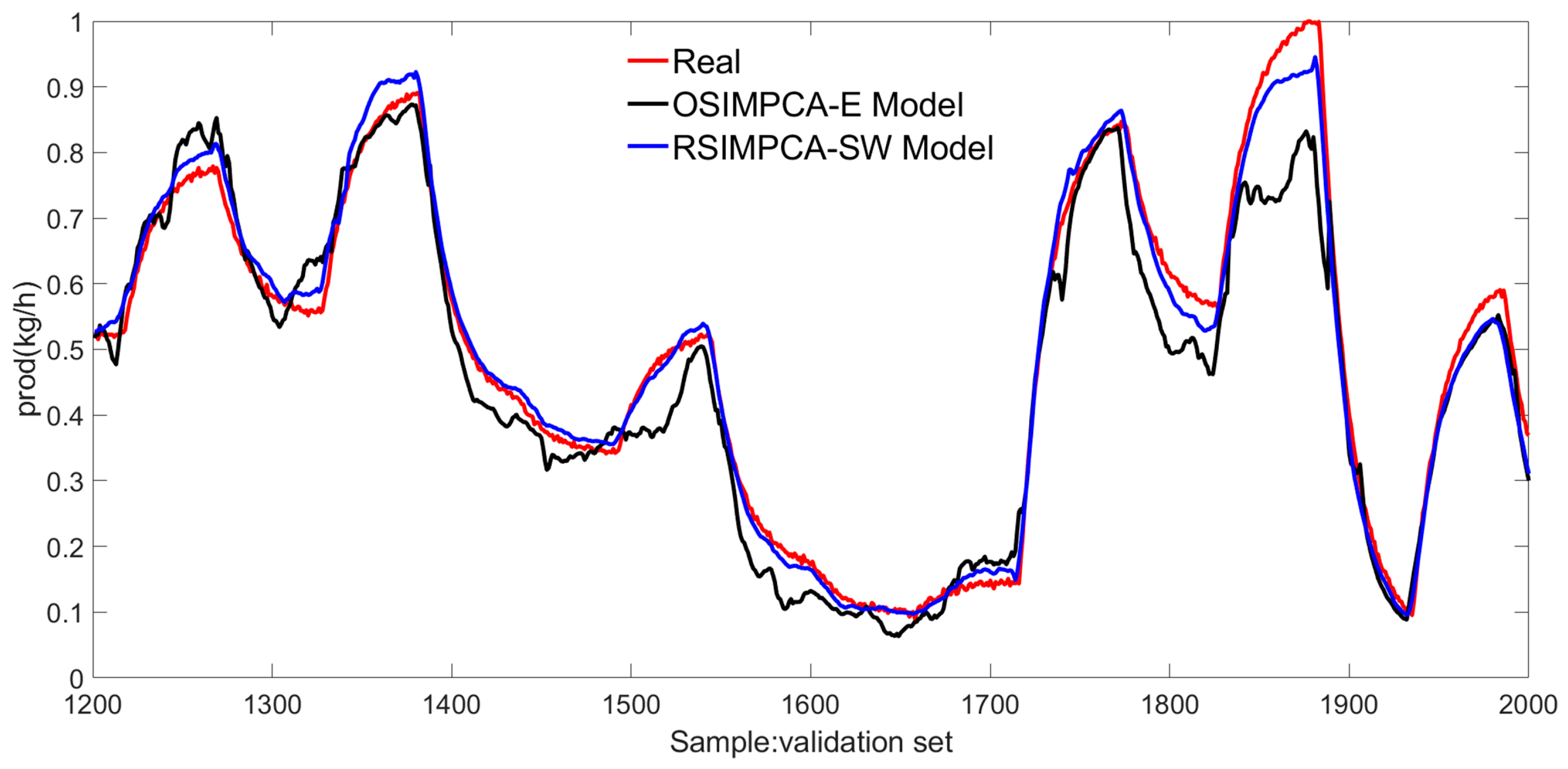
In order to test the performance of the RSIMPCA-SW model, the relevant predicted values and the real values are displayed in Figure 6 and Figure 7, further, where the OSIMPCA-E approach is introduced as the comparison.

Figure 6.
The response comparison of ppc2.
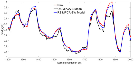
Figure 7.
The response comparison of prod.
5. Discussions
There are some general guidelines for the selection of the parameters for the proposed on-line subspace identification approach. In terms of the past and future horizons and , they will affect the dimensions of the relevant Hankel matrices, and their values must be bigger than the maximum order of the pre-set process model. For the selection of the optimal model order , it influences the relevant model identification precision greatly. As is mentioned in Section 4.3, the value of the corresponding MRSE can be chosen as the criterion. Note that although the MRSE values of some other orders may also be acceptable, the selection of the optimal order as 3 will offer a better compromise between model precision and the subsequent computation complexity.
By observing the statistical results for both approaches in Table 1, it can be easily seen that better identification performance is achieved for two on-line methods in which smaller RSE, MAE and bigger VAF are obtained. It is also implied that the recursion technology in on-line identification algorithms is beneficial for coping with various uncertainties in practice and complex characteristics in polymerization. Among the two on-line subspace identification schemes, the proposed RSIMPCA-SW algorithm shows superiority with improved statistical results in which RSE and MAE are smaller and VAF is larger. The corresponding responses of two on-line approaches are shown in Figure 6 and Figure 7. It can be found that the predicted values of the proposed strategy are closer to the actual values, comparing with those of the OSIMPCA-E approach, by and large, which also indicates that enhanced model identification precision is achieved for the proposed RSIMPCA-SW method. In a word, the proposed on-line scheme provides better ensemble identification performance.
Note that it is common to fill in the missing data using interpolation methods (e.g., linear interpolation and polynomial interpolation) during the data preprocessing stage. When a variable which needs to be modeled is not available, the other highly correlated variable will be chosen as the alternate. Then, the result of the alternate variable can be regarded as the related reference. For a polymerization processes with more variables, faster recursive computation speed and improved identification accuracy are also expected for the proposed algorithm because of the adoption of PCA and LQ decomposition with the bona fide method.
6. Conclusions
In this paper, a new on-line recursive subspace identification method based on PCA and sliding window is developed to obtain a more precise model with smaller computation complexity for polymerization. Compared with the conventional subspace methods, PCA is employed to improve the estimation precision of the extended observation matrix, and LQ decomposition with the bona fide method are also utilized for reducing the computation complexity of the recursion in the on-line identification. Based on the introduction of the above two technologies, improved identification precision and lower computation complexity are anticipated. At the same time, an optimal estimation method for the process model order under a recommended criterion is given. The case study of the model identification of the polyethylene process shows that smaller ensemble prediction errors were obtained for the proposed RSIMPCA-SW approach. Meanwhile, the VAF results and the related responses also imply that better fitting performance is gained for the proposed on-line algorithm. And all these above results verify the superiority of the proposed RSIMPCA-SW approach compared with the introduced off-line and on-line subspace identification algorithms.
Author Contributions
Conceptualization, J.Q., T.L. and G.H.; methodology, J.Q.; software, J.Q. and J.Z.; validation, J.Q., S.L. and C.S.; formal analysis, C.S. and S.L.; investigation, J.Q.; resources, J.Z.; data curation, J.Q. and S.L.; writing—original draft preparation, J.Q., T.L. and C.S.; writing—review and editing, J.Q., T.L. and G.H.; visualization, J.Q.; supervision, G.H. and B.W.; project administration, C.S. and G.H.; funding acquisition, J.Z., G.H. and B.W. All authors have read and agreed to the published version of the manuscript.
Funding
This research was funded by Zhejiang Provincial Science and Technology Plan Project, China (Grant No. 2023C01117).
Data Availability Statement
Data are available upon request due to privacy restrictions. The data presented in this study are available upon request from the corresponding author.
Conflicts of Interest
Authors Jubin Zhang and Bin Wen were employed by the company Hangzhou Sinan Intellitech Co., Ltd. The remaining authors declare that the research was conducted in the absence of any commercial or financial relationships that could be construed as a potential conflict of interest.
References
- Ray, W.H.; Villa, C.M. Nonlinear dynamics found in polymerization processes—A review. Chem. Eng. Sci. 2000, 55, 275–290. [Google Scholar] [CrossRef]
- Kreitser, T.; Tumina, S.; L’Vovskii, V. Effect of the parameters of the mathematical model of polymerization kinetics, on estimation of the molecular weight of polyethylene. Polym. Sci. U.S.S.R. 1978, 20, 2989–2998. [Google Scholar] [CrossRef]
- Vivaldo-Lima, E.; Mohammadi, Y.; Penlidis, A. Modeling and simulation of polymerization processes. Processes 2021, 9, 821. [Google Scholar] [CrossRef]
- Fiosina, J.; Sievers, P.; Drache, M.; Beuermann, S. Polymer reaction engineering meets explainable machine learning. Comput. Chem. Eng. 2023, 177, 108356. [Google Scholar] [CrossRef]
- Touloupidis, V. Catalytic Olefin Polymerization Process Modeling: Multi-Scale Approach and Modeling Guidelines for Micro-Scale/Kinetic Modeling. Macromol. React. Eng. 2014, 8, 508–527. [Google Scholar] [CrossRef]
- Bashir, M.A.; Kanellopoulos, V.; Ali, M.A.; McKenna, T.F. Applied Thermodynamics for Process Modeling in Catalytic Gas Phase Olefin Polymerization Reactors. Macromol. React. Eng. 2020, 14, 1900029. [Google Scholar] [CrossRef]
- Zhang, Z.; Guo, F.; Song, W.; Jia, X.; Wang, Y. Empirical correction of kinetic model for polymer thermal reaction process based on first order reaction kinetics. Chin. J. Chem. Eng. 2021, 38, 132–144. [Google Scholar] [CrossRef]
- Urrea-Quintero, J.-H.; Marino, M.; Hernandez, H.; Ochoa, S. Multiscale modeling of a free-radical emulsion polymerization process: Numerical approximation by the Finite Element Method. Comput. Chem. Eng. 2020, 140, 106974. [Google Scholar] [CrossRef]
- Mueller, P.A.; Richards, J.R.; Congalidis, J.P. Polymerization reactor Modeling in Industry. Macromol. React. Eng. 2011, 5, 261–277. [Google Scholar] [CrossRef]
- Tan, L.P.; Lotfi, A.; Lai, E.; Hull, J. Soft computing applications in dynamic model identification of polymer extrusion process. Appl. Soft Comput. 2004, 4, 345–355. [Google Scholar] [CrossRef]
- Lima, N.M.; Linan, L.Z.; Melo, N.C.; Manenti, F.; Filho, R.M.; Embirucu, M.; Maciel, R.W. Nonlinear fuzzy identification of batch polymerization processes. Comput. Aided Chem. Eng. 2015, 37, 599–604. [Google Scholar]
- Liu, Z.; Luan, X. Intelligent Modeling for Batch Polymerization Reactors with Unknown Inputs. Sensors 2023, 23, 6021. [Google Scholar] [CrossRef]
- Qin, S.J. An overview of subspace identification. Comput. Chem. Eng. 2006, 30, 1502–1513. [Google Scholar] [CrossRef]
- Corbett, B.; Mhaskar, P. Subspace identification for data-driven modeling and quality control of batch processes. AIChE J. 2016, 62, 1581–1601. [Google Scholar] [CrossRef]
- Ghosh, D.; Hermonat, E.; Mhaskar, P.; Snowling, S.; Goel, R. Hybrid Modeling Approach Integrating First-Principles Models with Subspace Identification. Ind. Eng. Chem. Res. 2019, 58, 13533–13543. [Google Scholar] [CrossRef]
- Lou, H.; Su, H.; Gu, Y.; Hou, W.; Xie, L.; Rong, G. Nonlinear predictive control with modified closed-loop subspace identifi-cation-piecewise linear model for double-loop propylene polymerization process. Control. Theory Appl. 2015, 32, 1040–1051. [Google Scholar]
- Verhaegen, M. Identification of the deterministic part of MIMO state space models given in innovations form from in-put-output data. Automatica 1994, 30, 61–74. [Google Scholar]
- Van Overschee, P.; De Moor, B. N4SID: Subspace algorithms for the identification of combined deterministic-stochastic systems. Automatica 1994, 30, 75–93. [Google Scholar]
- Hou, J.; Liu, T.; Chen, F. Orthogonal projection based subspace identification against colored noise. Control. Theory Technol. 2017, 15, 69–77. [Google Scholar] [CrossRef]
- Song, I.H.; Rhee, H.K. Nonlinear control of polymerization reactor by Wiener predictive controller based on one-step sub-space identification. Ind. Eng. Chem. Res. 2004, 43, 7261–7274. [Google Scholar]
- Gomes, F.P.C.; Garg, A.; Mhaskar, P.; Thompson, M.R. Data-Driven Advances in Manufacturing for Batch Polymer Processing Using Multivariate Nondestructive Monitoring. Ind. Eng. Chem. Res. 2019, 58, 9940–9951. [Google Scholar] [CrossRef]
- Mercère, G.; Bako, L.; Lecœuche, S. Propagator-based methods for recursive subspace model identification. Signal Process. 2008, 88, 468–491. [Google Scholar] [CrossRef]
- Shang, L.; Liu, J.; Zhang, Y.; Wang, G. Efficient recursive canonical variate analysis approach for monitoring time-varying processes. J. Chemom. 2017, 31, e2858. [Google Scholar] [CrossRef]
- Wu, P.; Chen, L.; Zhou, W.; Guo, L. Online subspace identification based on principal component analysis and noise estima-tion. J. Zhejiang Univ. 2018, 52, 1694–1701. [Google Scholar]
- Misra, S.; Nikolaou, M. Adaptive design of experiments for model order estimation in subspace identification. Comput. Chem. Eng. 2017, 100, 119–138. [Google Scholar] [CrossRef]
- Sugiyama, M.; Ogawa, H. Subspace Information Criterion for Model Selection. Neural Comput. 2001, 13, 1863–1889. [Google Scholar] [CrossRef]


Disclaimer/Publisher’s Note: The statements, opinions and data contained in all publications are solely those of the individual author(s) and contributor(s) and not of MDPI and/or the editor(s). MDPI and/or the editor(s) disclaim responsibility for any injury to people or property resulting from any ideas, methods, instructions or products referred to in the content. |
© 2024 by the authors. Licensee MDPI, Basel, Switzerland. This article is an open access article distributed under the terms and conditions of the Creative Commons Attribution (CC BY) license (https://creativecommons.org/licenses/by/4.0/).