The TPRF: A Novel Soft Sensing Method of Alumina–Silica Ratio in Red Mud Based on TPE and Random Forest Algorithm

Abstract

The online measurement of the aluminum–silicon ratio of red mud in the dissolution stage of the Bayer alumina production process is difficult to achieve. The offline assay method has a high cost and strong time delay. Soft sensors are an effective and economical method to solve such problems. In this paper, a hybrid model (TPRF model) based on a tree-structured Parzen estimator (TPE) optimized random forest (RF) algorithm is proposed to measure the Al–Si ratio of red mud. The probability distribution of the hyperparameters of the random forest model is estimated by combining the TPE optimization algorithm with the random forest algorithm. According to this probability distribution, the hyperparameters of the random forest algorithm are adjusted in the parameter search space to obtain the best combination of hyperparameters. We established a TPRF soft sensing model based on the optimal combination of hyperparameters. The results show that the best performance of the TPRF model is a mean absolute percentage error (MAPE) of 0.0015, a root-mean-square error (RMSE) of 0.00378, a mean absolute error (MAE) of 0.00162, and a goodness of fit ($R^2$) of 0.9893. The goodness of fit improved by 93.2% compared to the linear model, 39.1% compared to the SVR model, about 21.2% compared to the GRU model, and 5.5% compared to the RF model. This level of performance is demonstrated to be better than traditional soft sensors.

1. Introduction

In industrial production, some key production indicators cannot be measured and analyzed online through existing sensors [1]. It is usually necessary to take other means to obtain data, such as offline sampling and laboratory analysis [2]. However, the method of obtaining key production indexes by off-line assay and laboratory analysis is costly and has a strong lag [3]. Soft sensor technology uses easily measurable auxiliary variables to achieve an online real-time continuous estimation of unmeasurable or difficult-to-measure dominant variables. It has good inference and estimation ability and fast dynamic response ability [4], becoming a main online detection method for key production parameters in process industry processes [5].

According to the properties of soft sensor models, they can be divided into mechanistic-based soft sensor models and data-driven soft sensor models [6]. The data-driven soft sensor model does not require an analysis of the internal mechanisms of the controlled object. This model just uses input and output data to establish corresponding relationships. The model performs well in dealing with complex industrial processes with strong nonlinearity, especially in process industries such as metallurgy and chemical engineering. And it has become the main trend in building soft sensor models [7].

The LSTM model has excellent performance in processing sequence data and can effectively capture temporal correlations and patterns in the sequence. The model can prevent the problem of gradient disappearance or explosion through the use of a gating mechanism. The model performed well in certain tasks. Yuan, X., et al. [8] propose an LSTM model based on spatiotemporal attention to predict the boiling points of heavy oil and aviation kerosene in industrial hydrocracking processes. Ke, W., et al. [9] propose a deep neural network structure based on LSTM and apply it to practical cases of coal gasification, and the model performed well. Pan, H., et al. [10] propose a soft sensor model based on long short-term memory networks to predict the oxygen content in boiler flue gas. Hua, L., et al. [11] propose a new mixed soft sensor model based on RF-IHHO-LSTM for the penicillin fermentation process, which can monitor the parameter changes of the penicillin fermentation process in real time. Miettinen, J., et al. [12] propose a soft sensor based on bidirectional long short-term memory (LSTM) to predict the lateral displacement trajectory of the rotor, with an average absolute error (MAE) of 0.0063 mm. Yuan, X., et al. [13] propose a supervised LSTM (SLSTM) network for learning quality-related hidden dynamics in soft sensor applications.

Some scholars have conducted research on other soft sensor models. Yan, W., et al. [14] combined a denoising autoencoder with a neural network (DAE-NN) to predict the oxygen content in the flue gas of 1000 MW ultra-high efficiency units. Armaghani, D.J., et al. [15] propose a PSO-ANN model to predict the propulsion speed of tunnel boring machines in different granite weathering zones. Liao, Z., et al. [16] propose a multi-wavelet convolutional neural network (MWCNN) for load forecasting, and its performance was verified through experiments. Wang, X., et al. [17] propose a multi-objective evolutionary nonlinear ensemble learning model (MOENE-EFS) with an evolutionary feature selection mechanism to predict the silicon content in molten iron. Yuan, X., et al. [18] propose a new variable weighted stacked autoencoder (VW-SAE) and industrial applications have shown that this model can provide better performance. Nkulikiyinka, P., et al. [19] compared the gas concentration prediction performance in the reformer and regenerator reactors of the SE-SMR process; the random forest model showed better prediction performance. Arhab, M., et al. [20] use a random forest model to predict the levels of nitrate, orthophosphate, and ammonium in the Rhine River in Germany. Wan, Y., et al. [21] propose a random forest model based on an attention mechanism, and its performance is verified in practical industrial cases. Balakrishnan, R., et al. [22] propose an artificial-neural-network-based maximum-power-point-tracking scheme, and it is applied to maximize power generation from photovoltaic sources.

In this paper, a hybrid model (TPRF model) based on a tree-structured Parzen estimator (TPE) optimized Random Forest (RF) algorithm is proposed to measure the Al–Si ratio of red mud. This model solves the inherent nonlinear characteristics of time series data in industrial production and the problem of production information lag caused by off-line testing. It can effectively process datasets containing a large number of features and solve the interaction between different variables. By averaging the results of all regression trees, it is possible to stably handle missing data and outliers, reduce the impact of outliers on prediction results, and have good resistance to overfitting. In addition, the model only requires a small number of samples to achieve good predictive performance.

In this study, a new approach was proposed to solve practical engineering problems such as the difficulty and high cost of measuring the ratio of aluminum to silicon in red mud during the production of alumina by the Bayer process. By integrating the TPE optimization algorithm and random forest algorithm, the hyperparameter combination of the random forest algorithm is redesigned. A new hyperparameter is formed by coupling the structural parameters of the model with the parameters related to the Al–Si ratio of the red mud. Finally, the TPRF model is constructed through the improved hyperparameters. However, due to the limitation of actual production conditions, the stability of this model could not be verified in other alumina production environments. This limitation will be the focus of future research.

2. Research Method

2.1. TPE Model

Tree-structured Parzen estimator (TPE) is a sequential model based on global optimization (SMBO) algorithm. The proposed approach employs a tree structure to effectively model and optimize the intricate relationships among hyperparameters, thereby efficiently addressing multidimensional hyperparameter optimization problems. By utilizing the TPE algorithm, the optimal combination of hyperparameters can be obtained through a limited number of iterations, making it particularly suitable for scenarios with constrained computational resources. Its optimization mechanism, based on a tree structure, efficiently addresses multidimensional hyperparameter optimization problems.

For $p(x|y)$, the TPE algorithm adopts a different modeling method from other optimization methods, adopting a strategy of co-modeling $p(x|y)$ and $p(y)$, and expressing $p(x|y)$ in two density function forms:

$$p(x|y)=\left\{\begin{array}{c}l(x),y<y^{*}\hfill \\ g(x),y\ge y^{*}\hfill \end{array}\right.$$

(1)

x is the observation point; y is the observed value; y* is the threshold, usually the median of known observations; TPE optimization first clarifies y* based on existing observation points, and then divides the observation points into two probability density functions. l(x) is the probability density of the $\left\{x_{(i)}\right\}$ set corresponding to the observation value y being less than y*; g(x) is the probability density of the $\left\{x_{(i)}\right\}$ set corresponding to the observation value y being greater than or equal to y*.

TPE optimization utilizes the expected improvement (EI) acquisition strategy to form new observation points by maximizing EI. In order to optimize the TPE collection function of EI better and make $p(y)\ast p(x|y)$ equivalent to $p(x,y)$, the collection function EI of TPE is the following:

$$E{I}_{y^{*}}(x)={\displaystyle {\int }_{-\infty }^{y^{*}}\left(y^{*}-y\right)}p(y|x)dy={\displaystyle {\int }_{-\infty }^{y^{*}}\left(y^{*}-y\right)}\frac{p(x|y)p(y)}{p(x)}dy$$

(2)

When $\gamma =p(y<y^{\ast })$, $p(x)=\gamma l(x)+(1-\gamma )g(x)$, then

$${\displaystyle {\int }_{-\infty }^{y^{\ast }}(y^{\ast }-y)p(x|y)p(y)dy=l(x){\displaystyle {\int }_{-\infty }^{y^{\ast }}(y^{\ast }-y)}}p(y)dy=\gamma y^{\ast }l(x)-l(x){\displaystyle {\int }_{-\infty }^{y^{\ast }}p(y)dy}$$

(3)

Ultimately, the following can be concluded:

$$E{I}_{y^{*}}(x)=\frac{\gamma y\ast l(x)-l(x){\displaystyle {\int }_{-\infty }^{y^{\ast }}p(y)dy}}{\gamma l(x)+(1-\gamma )g(x)}\infty {(\gamma +\frac{g(x)}{l(x)}(1-\gamma ))}^{-1}$$

(4)

According to the equation above, during the process of maximizing expectations, when the hyperparameter x reaches its maximum probability l(x) and minimum probability g(x), the EI value is maximized. The TPE method utilizes l(x) and g(x) to construct a sample set of hyperparameters and evaluates x using g(x)/l(x). At each iteration, select the point with the highest EI value. This approach aims to balance development and exploration in order to seek overall optimal hyperparameters. In the hyperparameter optimization process of the TPRF model, a new hyperparameter x is used for constructing the TPRF model. Subsequently, training yields an observation value y which is compared with original observation values. The probability surrogate model is then updated to further optimize results.

2.2. Random Forest Model

Random forest was proposed by Breiman in 2001 and is an important and useful ensemble learning method. As a typical ensemble learning method, when performing regression tasks, random forest generates and integrates multiple regression decision trees based on Bagging strategy and Bootstrap sampling method to build a more powerful model, as shown in Figure 1.

The establishment of a decision tree usually includes three parts: feature selection, decision tree generation, and pruning. The selection indicators for features usually include information gain, information gain ratio, or Gini index, all of which can approximately represent the classification error rate.

The random forest algorithm can not only synthesize multiple input features to drive the model, but also calculate the relative importance of input features to the model. As an integrated learning algorithm, random forest algorithm can eliminate abnormal data by integrating the decision results of multiple decision trees, which provides a possibility for further optimization of input features and improvement of model accuracy. As a basic unit of random forest, decision tree has good generalization ability, which can not only complete the classification task, but also apply to regression problems. Assuming that the original data set is D, we randomly extract the sample data n times with replacement; j samples are extracted each time, from which n subsample sets d of size j are obtained. At the same time, there are M feature variables, and n random selections of k feature variables are made each time to obtain n feature variable quantum sets m. n regression decision trees are constructed by using subsets generated from the original data, and the average of the predicted values of these decision trees is taken as the final output of the random forest. The extraction of the sub-data sets is random, which can reduce the correlation between each tree and reduce the persistent generalization error, so as to ensure the accuracy and stability of the random forest model.

Regression decision tree is constructed by using a top-down strategy to recursively partition the target variable, with the core goal being to find the optimal segmentation rule through the selection of feature variables and the decision of segmentation points. Its construction process is based on dividing the target variable space into regions using feature variables:

$$d=\left[d_1,d_2,d_3\cdots \cdots d_j\right]$$

(5)

$$m=\left\{\begin{array}{l}{m}_1=\left[m_{11},m_{12}LL{m}_{1j}\right]\\ m_2=\left[m_{21},m_{22}LL{m}_{2j}\right]\\ m_3=\left[m_{31},m_{32}LL{m}_{3j}\right]\\ ⋮\\ m_k=\left[m_{k1},m_{k2}LL{m}_{kj}\right]\end{array}\right.$$

(6)

According to m feature variables, we can recursively perform binary splits on the sample set d. Each split considers only one feature variable and generates a binary tree. Eventually, the sample space R is partitioned into multiple non-overlapping subspaces R₁, R₂, …, R_r, corresponding to the leaf nodes of the tree. The mean of the sample values in each subspace is used as the numerical value for that space. When forecasting, points assigned to a subspace will predict the value of that subspace.

The criterion for each partition is to minimize the residual sum of squares of the sample values in each subspace and to continue until the stop condition is reached. Although the greedy method can find the optimal partitioning rules for each node in the regression decision tree, it is difficult to ensure the global optimality of the regression decision tree. In addition, individual regression decision trees are often very sensitive to perturbations in the data, which can lead to high variability in the predictions.

Ensemble methods such as random forests can transform weak learners into strong ensemble learners to solve the challenges faced by regression decision trees. Using multiple randomly generated regression decision trees can reduce overfitting and sensitivity to outliers to some extent. In order to estimate the generalization error of the model, an out-of-pocket estimation method is introduced, which can give unbiased estimates without using external data sets.

In addition, the importance of feature variables in model construction is evaluated by the way the prediction accuracy decreases when one feature variable is replaced while the other variables remain unchanged.

Compared with traditional random forest methods that deal with a single target variable, multivariate random forest (MRF) can realize the combined prediction of multiple target variables and take into account the potential dependencies between the target variables. In the regression task, multi-variable random forest uses Bagging and Bootstrap to construct multiple regression decision trees. The principle of extraction of original data and generation of regression decision trees is exactly the same as that of traditional random forest. The difference is that the target variables change from one-dimensional to multidimensional. Taking the prediction of the aluminum–silicon ratio of red mud as an example, compared to using RF to independently model and predict the input AO, input Si, circulating mother liquor flow rate, dissolution temperature, circulating mother liquor Rp, feed solid content, and dissolution Rp, or to independently model and predict the results obtained after logarithmic ratio conversion. MRF can simultaneously input the above relevant parameters to achieve synchronous prediction of aluminum–silicon ratio. Each sample contains seven types of information: incoming grinding AO, incoming grinding Si, circulating mother liquor flow rate, dissolution temperature, circulating mother liquor Rp, incoming solid content, and dissolution Rp. Therefore, the input target variable is a seven-dimensional vector. Represented by d₁, d₂, d₃… d₇, the subset of samples d* extracted during model construction can be expressed as the following:

$$d^{*}=\left[\left[d_{11},d_{21}\cdots \cdots d_{71}\right],\left[d_{12},d_{22}\cdots \cdots d_{72}\right],\cdots \cdots \left[d_{1j},d_{2j}\cdots \cdots d_{7j}\right]\right]$$

(7)

Decision tree algorithm has a natural advantage when dealing with multiple target variables. Different from the single variable regression decision tree, the sample division of the multivariable regression decision tree is based on the sum of the square residuals of seven data (d₁, d₂… d₇). This method to some extent considers the potential relationship between component data and also reflects the overall impact of characteristic variables on the aluminum–silicon ratio of red mud. It is worth noting that the prediction results of multi-output regression decision trees on component data may more naturally conform to the characteristics of component data. For multi-output regression trees, the prediction result is based on the mean of the samples in the divided sample space. Therefore, for the prediction results of Al–Si ratio of red mud, the multi-output regression tree can be consistent with the input results, maintain non-negative and the sum is 100%. In addition, MRF (multidimensional random forest) also uses the mean value strategy to process the results of multivariate regression decision trees, which makes the model more stable in performance.

Data samples with characteristics and red mud Al–Si ratios were collected, and the training set and test set were divided. Each sample contains two sets of elements, a feature and a label. The random forest algorithm is used to train and predict the model. In the training process, the random forest selects a part of the sample in a random way for modeling. This randomness helps reduce the variance of the model and increases robustness. Finally, the model is validated and tested with test set samples to evaluate its performance.

2.3. TPRF Model

The TPRF model framework can be divided into two main parts: the TPE hyperparameter optimization part and the random forest prediction part, as shown in Figure 2. The hyperparameter optimization part of TPE is mainly based on the fitness y of the prediction model of the historical iteration (generally the error of the prediction model in the virtual prediction period); the model hyperparameter x of the next iteration is obtained through optimization and solution, and then sent into the random forest prediction model to obtain the corresponding fitness y of the prediction model, and then sent back to the TPE model for hyperparameter optimization. This is repeated until the number of iterations or fitness y meets the prediction requirements.

3. Data Preprocessing

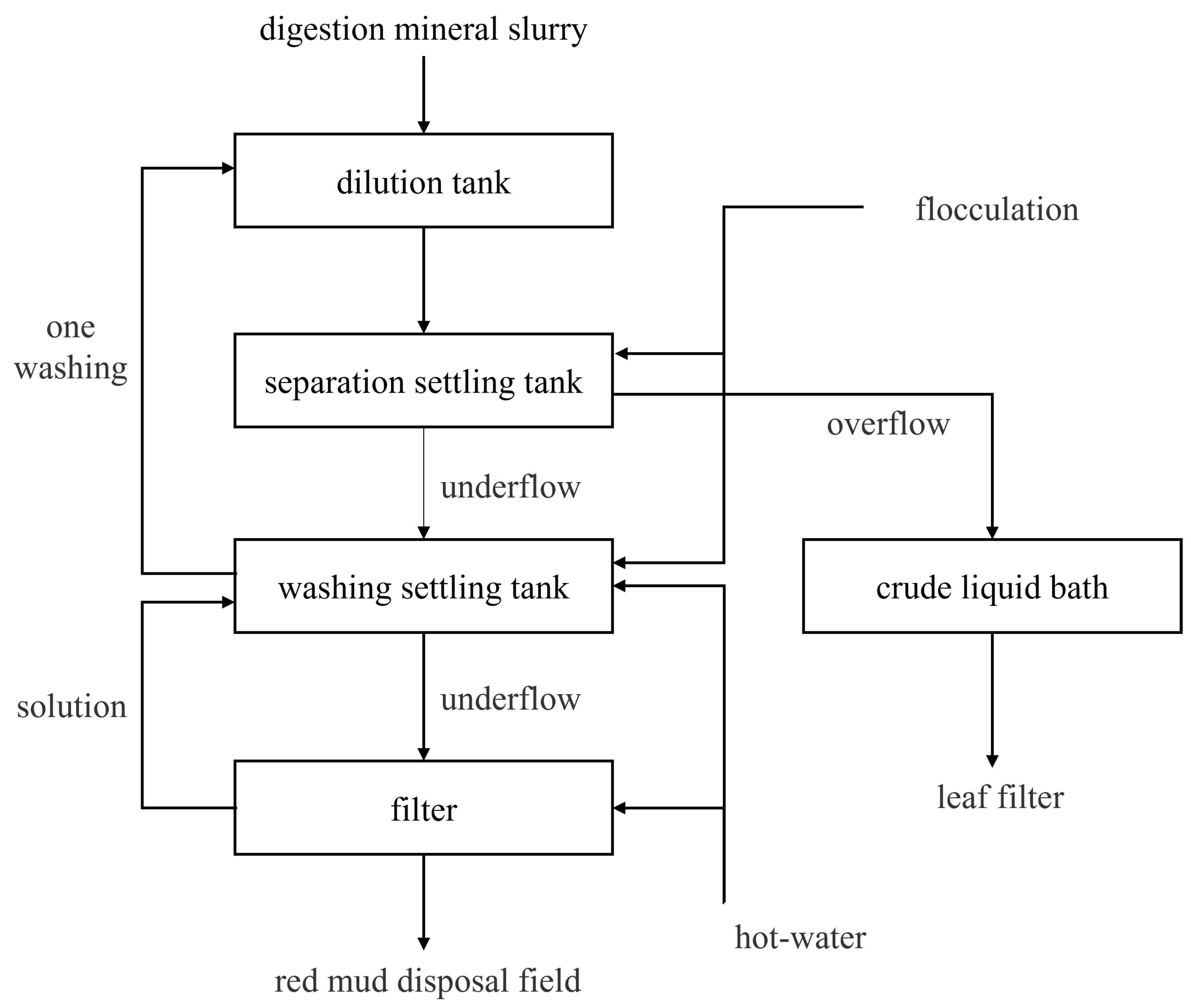
3.1. Data Collection and Determination of Associated Variables

Due to the harsh production environment, it is difficult for sensors and other measuring equipment to achieve the online measurement of key indicators in the dissolution stage of alumina production. All key data are obtained through offline testing and recorded in the ledger. Therefore, the data ledger of the dissolution process can provide a substantial amount of reliable experimental data for the experiment.

Based on the analysis of the collected experimental data, the dissolution stage mechanism of alumina production by the Bayer method is presented, as shown in Figure 3. Several relevant variables that could potentially impact the Al to Si ratio in red mud were screened, including grinding AO, grinding Si, circulating mother liquor flow rate, dissolution temperature, circulating mother liquor Rp value, feed solid content, and dissolution Rp value. The seven parameters were subjected to grey relational degree analysis.

Grey system theory introduces the concept of grey relational degree analysis for each subsystem, with the objective of identifying the quantitative relationship between subsystems (or factors) within the system using specific methods. It primarily focuses on describing the relative changes in magnitude and rate between the dependent variable index and the independent variable index during the continuous evolution of an environmental system. When the two indicators exhibit a similar change trend, the correlation between them is considered high. Conversely, if the change trend differs significantly, the correlation is regarded as low.

Through normalization methods, such as maximum–minimum normalization, the effect of dimensionality in each parameter is eliminated, and the original data are transformed into a dimensionless comparable sequence. Write the parent sequence as the $Y_o(t)$, let $Y_o(t)$ = $\left\{y_o(1),y_o(2),\cdots \cdots y_o(m)\right\}$, write the subsequence as the $Y_g(t)$, and let $Y_g(t)$ = $\left\{y_g(1),y_g(2),\cdots \cdots y_g(m)\right\}$. When $t=h$, the correlation coefficient between the parent sequence $Y_o(t)$ and the subsequence $Y_g(t)$ is ${\xi }_{og}(h)$,

$${\xi }_{og}(h)=\frac{{\Delta }_{\min }+\rho {\Delta }_{\max }}{{\Delta }_{og}(h)+\rho {\Delta }_{\max }}$$

(8)

${\Delta }_{og}(h)$ is the absolute difference of the pairwise comparison sequence of the h group data. ${\Delta }_{\max }$ and ${\Delta }_{\min }$ are the maximum and minimum values of the absolute difference of each comparison sequence in each group of data. And $\rho$ is the resolution coefficient, which is generally 0.1 to 0.5.

$${\gamma }_{og}=\frac{1}{m}{\displaystyle \sum _{h=1}^m{\xi }_{og}(h)}$$

(9)

${\gamma }_{og}$ is the correlation degree between the parent sequence o and subsequence g.

Parameter 0 refers to the grinding AO, parameter 1 refers to the grinding Si, parameter 2 refers to the flow rate of circulating mother liquor, parameter 3 refers to the dissolution temperature, parameter 4 refers to the circulating mother liquor Rp, parameter 5 refers to the feed solid content, parameter 6 refers to the dissolution Rp, and parameter 7 refers to the ratio of aluminum to silicon in red mud. The data set number column serves as the main sequence, while the data set numbers of other parameters are listed as sub-sequences. The correlation between the parameters is calculated based on the aforementioned steps, and the calculation results are shown in Figure 4.

As can be seen from Figure 4, the correlation degree between the above parameters and the Al–Si ratio of red mud exceeds 0.6. Moreover, the difference between the correlation degrees of the other parameters is also small. It is sufficient to prove that there is an obvious correlation between the above parameters and the Al–Si ratio of red mud. Therefore, the above seven parameters are selected as input variables.

The specific model input variable parameters are shown as

Table 1. The model input variable.

Input variables
Number	Variable	Unit	Number	Variable	Unit
1	Grinding AO	t	5	Circulating mother liquor Rp	%
2	Grinding Si	t	6	Feed solid content	$\mathrm{g}/\mathrm{L}$
3	Dissolution temperature	$°\mathrm{C}$	7	Dissolution Rp	%
4	Circulating mother liquor flow rate	${\mathrm{m}}^3/\mathrm{L}$
Target variable
Number	Variable	Unit	Number	Variable	Unit
1	Red mud aluminum–silicon ratio	%

, as follows:

3.2. Outlier Determination and Missing Value Padding

The authenticity and reliability of the source data are critical in developing a soft model for predicting the aluminum–silicon ratio of dissolved red mud in alumina production. The source data is collected through offline laboratory testing, which involves a random sampling process. However, it is important to acknowledge that errors can occur during the laboratory testing phase due to factors such as improper operation or limitations in the measuring equipment. These errors can lead to significant discrepancies between the measured data and the actual data, which can subsequently impact the quality of the database and compromise the accuracy of the red mud aluminum–silicon ratio soft sensor model.

To address these challenges and enhance the quality of the input variables, appropriate data preprocessing methods need to be employed. Outlier removal techniques can help identify and eliminate data points that deviate significantly from the expected range, thereby reducing the influence of erroneous measurements. Additionally, missing value-filling methods can be applied to address any gaps or missing data points in the collected source data. By effectively addressing outliers and missing values, the overall quality of the input variables can be improved, leading to more accurate predictions from the red mud aluminum–silicon ratio soft sensor model.

Common methods for detecting outliers include statistical analysis and $3\sigma$ principles, and box plots. This study adopts the 3σ principle to determine outliers.

The $3\sigma$ principle is that random errors exist in the obtained source data, and the mean $\mu$ and standard deviation $\sigma$ are obtained by processing the source data.

$$\mu =\frac{{\displaystyle \sum _{i=1}^n{x}_i}}{n}$$

(10)

$$\sigma =\sqrt{\frac{{\displaystyle \sum _{i=l}^n{(x_i-\mu )}^2}}{n}}$$

(11)

A normal value interval $(\mu -3\sigma ,\mu +3\sigma )$ is determined according to the probability. When a certain datum in the sample exceeds this interval, it is not a random error but a gross error. The sample datum containing this error should be removed to leave more representative data to optimize the performance of the model.

After eliminating the outliers through the decision strategy, a portion of the sample data will be missing, thereby impacting the integrity of the database. Common preprocessing techniques for handling missing data include mean imputation, median imputation, mode imputation, etc. In this experiment, mean imputation was employed to ensure the authenticity and reliability of the data.

3.3. Data Normalization

In this paper, seven associated variables, namely grinding AO, grinding Si, circulating mother liquor flow rate, dissolution temperature, circulating mother liquor Rp value, feed solid content, and dissolution Rp value, were selected as the input data. However, different variables often have different dimensions and dimensional units, which affect the analysis results of the data. Through data normalization processing, the data are in the same order of magnitude after processing, so that the data indicators are comparable.

The commonly used data normalization methods are Z-Score normalization and min–max normalization, etc. In this paper, min–max normalization is adopted.

Min–max normalization is a linear transformation of the data, mapping the result to [0, 1].

$$x^{*}=\frac{x_i-x_{\min }}{x_{\max }-x_{\min }}$$

(12)

$x_{\max }$ is the maximum value in the sample data, and $x_{\min }$ is the minimum value in the sample data.

The obtained source data were analyzed and collated to determine the main factors affecting the Al–Si ratio of red mud. The sample data set was obtained through data preprocessing methods such as outliers judgment, missing value-filling, and data normalization. An amount of 80% of the sample data set was used as the training set of the red mud Al–Si ratio soft-sensor model, and 20% of the data set was used as the test set to verify the accuracy of the model.

4. Result and Discussion

4.1. The Result of the Model Prediction

According to the experimental results, several regression models are investigated and the test data are compared. The linear regression model, support vector regression model, random forest regression model, and TPRF model were used, respectively. The performance of each model is observed by looking at a graph comparing the true value with the predicted value. Moreover, the application of a recurrent neural network (RNN) is considered. Compared with the LSTM and traditional RNN models, GRU models have memory units similar to LSTM, but the number of parameters is less, and the calculation is more efficient. The GRU model performs relatively better when dealing with long sequences because it is better able to capture long-term dependencies. Therefore, the GRU model is chosen as the comparison model in this engineering problem. The comparison between the real value and the test value is shown in Figure 5, Figure 6, Figure 7, Figure 8 and Figure 9.

4.2. Evaluation of Performance Indication

The performance of the above models was evaluated by the performance index function. The mean absolute percentage error (MAPE), goodness of fit (R²), root-mean-square error (RMSE), mean absolute error (MAE), and relative error (RE) were selected to evaluate the prediction accuracy of the linear regression model, support vector regression model (SVR), recurrent neural network model, and random forest regression model. The values of each error evaluation index are shown in

Table 2. Valuation of model performance indicators.

Model	MAPE/%	RMSE/%	MAE	${\mathit{R}}^2$
Linear	0.0237	0.03455	0.02634	0.0672
SVR	0.0153	0.02201	0.01705	0.6023
GRU	0.0117	0.01664	0.01291	0.7800
RF	0.0036	0.00908	0.00397	0.9344
TPRF	0.0015	0.00378	0.00162	0.9893

.

(1). Mean absolute percentage error

$$MAPE=\frac{1}{n}\ast {\displaystyle \sum _{i=1}^n|}\frac{y_i^{*}-y_i}{y_i}|\ast 100\%$$

(13)

(2). R-square

$$R^2=1-\frac{{\displaystyle \sum _{i=1}^{16}{(y_i^4-y_i)}^2}}{{\displaystyle \sum _{i=1}^{16}{(y_i-\overline{y})}^2}}$$

(14)

(3). Root-mean-square error

$$RMSE=\sqrt{\frac{1}{n}·{\displaystyle \sum _{i=1}^n{(y_i^{*}-y_j)}^2}}$$

(15)

(4). Mean absolute error

$$MAE=\frac{1}{n}\ast {\displaystyle \sum _{i=1}^n|}{y}_i^{*}-y_i|$$

(16)

In the above formula, n is the number of samples in the sample set, $y_i^{*}$ is the predicted value of the model, and $y_i$ is the real value of the model input. The mean of the input values to the model is measured, and $\overline{y}$ is the mean of the input values.

The error evaluation indexes among all models are shown in Figure 10.

4.3. Model Performance Comparison

Through the comparison chart and Table 2 of the above real values and predicted values, it can be seen that the prediction effect of the linear regression model is poor. In most of the sample data, there is a significant discrepancy between the predicted values and the real values. Particularly, when the sample data undergoes changes, the model fails to accurately identify and incorporate these changes, resulting in considerable errors in the prediction results. Figure 3 and Figure 8, and Table 2 clearly demonstrate that the linear model has a low prediction accuracy, with an MAPE (mean absolute percentage error) of 0.0237, RMSE (root-mean-square error) of 0.03455, and MAE (mean absolute error) of 0.02634. These metrics indicate that the linear regression model performs the worst among the five models evaluated. Moreover, the $R^2$ of the tested value and the true value is only 0.0672, resulting in a poor fitting effect.

The prediction performance index of the SVR model was evaluated (MAPE = 0.0153, RMSE = 0.02201, MAE = 0.01705, $R^2$ = 0.6023), which was significantly improved compared with the linear model. Since the linear model is a linear regression model, the polynomial regression processing ability for nonlinear data or the correlation between data features is low. However, in the construction of the red mud Al–Si ratio model, there is a large amount of data, strong nonlinear relationship, multiple input data, each input data is correlated with each other, and the coupling is strong, resulting in the linear model’s weak generalization ability, poor fitting effect, and large prediction error. The SVR model transforms the actual problem to be solved into a low-dimensional characteristic vector through nonlinear mapping, and then projects it into a high-dimensional space to generate an optimal hyperplane meeting the requirements in the high-dimensional region. This property ensures that the model itself has good generalization performance and improves the prediction accuracy of the model.

The evaluation results of the predictive performance indexes of the GRU model are MAPE = 0.0117, RMSE = 0.01664, MAE = 0.01291, and $R^2$ = 0.7800, which has a certain improvement compared with the above two models. The GRU (gated recurrent unit) model simplifies the gate structure. In the GRU model, there are two main gates: the update gate and the reset gate. By using these gates, the GRU model effectively addresses the issues of vanishing gradients and exploding gradients commonly faced in traditional recurrent neural networks. Additionally, the GRU model introduces a linear dependency between the current state and the previous state, which helps in capturing long-term dependencies in the data. This linear dependency provides a balance between maintaining important information from the past and incorporating new information.

The RF model is an important and useful ensemble learning method. In the regression task, multiple regression decision trees are generated and integrated based on the Bagging strategy and Bootstrap sampling method. Finally, the prediction result is obtained. The predictive performance index evaluation results of the RF model were MAPE = 0.0036, RMSE = 0.00908, MAE = 0.00397, and $R^2$ = 0.9344, which were improved by 69%, 45%, 69%, and 20%, respectively, compared with the GRU model.

By combining the TPE model and RF model, the PRF model uses a tree structure to represent the relationship between hyperparameters, maps each parameter to a high-dimensional space, and uses the expected improvement (EI) acquisition strategy to find the optimal hyperparameters of the RF model in the process of optimizing EI values. This model efficiently solves the multi-dimensional optimization problem. Finding the optimal RF model hyperparameters makes the RF model learn the sample data better, ensures the model itself has good generalization performance, and improves the model prediction accuracy. The evaluation results of predictive performance indexes of the TPRF model were MAPE = 0.0015, RMSE = 0.00378, MAE = 0.00162, and $R^2$ = 0.9893.

5. Conclusions

In this paper, a TPE optimization algorithm is combined with a random forest algorithm to predict the Al to Si ratio of red mud in the Bayer process. It has contributed to reducing the cost of testing and helping industrial production realize the real-time monitoring of the aluminum–silicon ratio content in red mud. In this study, a hybrid model (TPRF model) based on the combination of a TPE algorithm and a random forest algorithm is proposed to measure the aluminum–silicon ratio of red mud. The results show that the best performance of the TPRF model is the mean absolute percentage error (MAPE) of 0.0015, the root-mean-square error (RMSE) of 0.00378, the mean absolute error (MAE) of 0.00162, and the goodness of fit ($R^2$) of 0.9893. The goodness of fit improved by 93.2% compared to the linear model, by 39.1% compared to the SVR model, by about 21.2% compared to the GRU model, and by 5.5% compared to the RF model, making this approach better than traditional soft sensors. The results show that the aluminum–silicon ratio of red mud can be accurately predicted by the model through input variables, so as to obtain the dissolution efficiency of aluminum in the production process in real time, allowing producers to adjust production in real time.

References

1. Liu, C.; Wang, K.; Wang, Y.; Yuan, X. Learning Deep Multimanifold Structure Feature Representation for Quality Prediction with an Industrial Application. IEEE Trans. Ind. Inform. 2022, 18, 5849–5858. [Google Scholar] [CrossRef]
2. Yuan, X.; Gu, Y.; Wang, Y.; Yang, C.; Gui, W. A Deep Supervised Learning Framework for Data-Driven Soft Sensor Modeling of Industrial Processes. IEEE Trans. Neural Netw. Learn. Syst. 2020, 31, 4737–4746. [Google Scholar] [CrossRef]
3. Ren, L.; Meng, Z.; Wang, X.; Zhang, L.; Yang, L.T. A Data-Driven Approach of Product Quality Prediction for Complex Production Systems. IEEE Trans. Ind. Inform. 2021, 17, 6457–6465. [Google Scholar] [CrossRef]
4. Perera, Y.S.; Ratnaweera, D.A.A.C.; Dasanayaka, C.H.; Abeykoon, C. The Role of Artificial Intelligence-Driven Soft Sensors in Advanced Sustainable Process Industries: A Critical Review. Eng. Appl. Artif. Intell. 2023, 121, 105988. [Google Scholar] [CrossRef]
5. Curreri, F.; Patanè, L.; Xibilia, M.G. RNN- and LSTM-Based Soft Sensors Transferability for an Industrial Process. Sensors 2021, 21, 823. [Google Scholar] [CrossRef]
6. Zhou, P.; Wang, X.; Chai, T. Multiobjective Operation Optimization of Wastewater Treatment Process Based on Reinforcement Self-Learning and Knowledge Guidance. IEEE Trans. Cybern. 2023, 53, 6896–6909. [Google Scholar] [CrossRef]
7. Sun, Y.-N.; Qin, W.; Hu, J.-H.; Xu, H.-W.; Sun, P.Z.H. A Causal Model-Inspired Automatic Feature-Selection Method for Developing Data-Driven Soft Sensors in Complex Industrial Processes. Engineering 2023, 22, 82–93. [Google Scholar] [CrossRef]
8. Yuan, X.; Li, L.; Shardt, Y.A.W.; Wang, Y.; Yang, C. Deep Learning with Spatiotemporal Attention-Based LSTM for Industrial Soft Sensor Model Development. IEEE Trans. Ind. Electron. 2021, 68, 4404–4414. [Google Scholar] [CrossRef]
9. Ke, W.; Huang, D.; Yang, F.; Jiang, Y. Soft Sensor Development and Applications Based on LSTM in Deep Neural Networks. In Proceedings of the 2017 IEEE Symposium Series on Computational Intelligence (SSCI), Honolulu, HI, USA, 27 November–1 December 2017; IEEE: Piscataway, NJ, USA, 2017; pp. 1–6. [Google Scholar]
10. Pan, H.; Su, T.; Huang, X.; Wang, Z. LSTM-Based Soft Sensor Design for Oxygen Content of Flue Gas in Coal-Fired Power Plant. Trans. Inst. Meas. Control 2021, 43, 78–87. [Google Scholar] [CrossRef]
11. Hua, L.; Zhang, C.; Sun, W.; Li, Y.; Xiong, J.; Nazir, M.S. An Evolutionary Deep Learning Soft Sensor Model Based on Random Forest Feature Selection Technique for Penicillin Fermentation Process. ISA Trans. 2023, 136, 139–151. [Google Scholar] [CrossRef]
12. Miettinen, J.; Tiainen, T.; Viitala, R.; Hiekkanen, K.; Viitala, R. Bidirectional LSTM-Based Soft Sensor for Rotor Displacement Trajectory Estimation. IEEE Access 2021, 9, 167556–167569. [Google Scholar] [CrossRef]
13. Yuan, X.; Li, L.; Wang, Y. Nonlinear Dynamic Soft Sensor Modeling with Supervised Long Short-Term Memory Network. IEEE Trans. Ind. Inform. 2020, 16, 3168–3176. [Google Scholar] [CrossRef]
14. Yan, W.; Tang, D.; Lin, Y. A Data-Driven Soft Sensor Modeling Method Based on Deep Learning and Its Application. IEEE Trans. Ind. Electron. 2017, 64, 4237–4245. [Google Scholar] [CrossRef]
15. Armaghani, D.J.; Koopialipoor, M.; Marto, A.; Yagiz, S. Application of Several Optimization Techniques for Estimating TBM Advance Rate in Granitic Rocks. J. Rock Mech. Geotech. Eng. 2019, 11, 779–789. [Google Scholar] [CrossRef]
16. Liao, Z.; Pan, H.; Fan, X.; Zhang, Y.; Kuang, L. Multiple Wavelet Convolutional Neural Network for Short-Term Load Forecasting. IEEE Internet Things J. 2021, 8, 9730–9739. [Google Scholar] [CrossRef]
17. Wang, X.; Hu, T.; Tang, L. A Multiobjective Evolutionary Nonlinear Ensemble Learning with Evolutionary Feature Selection for Silicon Prediction in Blast Furnace. IEEE Trans. Neural Netw. Learn. Syst. 2022, 33, 2080–2093. [Google Scholar] [CrossRef] [PubMed]
18. Yuan, X.; Huang, B.; Wang, Y.; Yang, C.; Gui, W. Deep Learning-Based Feature Representation and Its Application for Soft Sensor Modeling with Variable-Wise Weighted SAE. IEEE Trans. Ind. Inform. 2018, 14, 3235–3243. [Google Scholar] [CrossRef]
19. Nkulikiyinka, P.; Yan, Y.; Güleç, F.; Manovic, V.; Clough, P.T. Prediction of Sorption Enhanced Steam Methane Reforming Products from Machine Learning Based Soft-Sensor Models. Energy AI 2020, 2, 100037. [Google Scholar] [CrossRef]
20. Arhab, M.; Huang, J. Determination of Optimal Predictors and Sampling Frequency to Develop Nutrient Soft Sensors Using Random Forest. Sensors 2023, 23, 6057. [Google Scholar] [CrossRef]
21. Wan, Y.; Liu, D.; Ren, J.-C. A Modeling Method of Wide Random Forest Multi-Output Soft Sensor with Attention Mechanism for Quality Prediction of Complex Industrial Processes. Adv. Eng. Inform. 2024, 59, 102255. [Google Scholar] [CrossRef]
22. Balakrishnan, R.; Geetha, V.; Kumar, M.R.; Leung, M.-F. Reduction in Residential Electricity Bill and Carbon Dioxide Emission through Renewable Energy Integration Using an Adaptive Feed-Forward Neural Network System and MPPT Technique. Sustainability 2023, 15, 14088. [Google Scholar] [CrossRef]
Figure 1. Random forest model.
Processes 12 00663 g001
Figure 2. TPRF model.
Processes 12 00663 g002
Figure 3. Production process diagram.
Processes 12 00663 g003
Figure 4. Gray Relational Matrix Heatmap.
Processes 12 00663 g004
Figure 5. Prediction Results of Multiple Linear Regression Model.
Processes 12 00663 g005
Figure 6. Prediction Results of SVR Model.
Processes 12 00663 g006
Figure 7. Prediction Results of GRU Model.
Processes 12 00663 g007
Figure 8. Prediction Results of Random Forest Model.
Processes 12 00663 g008
Figure 9. TPRF Model Prediction Results.
Processes 12 00663 g009
Figure 10. Error evaluation index of each model.
Processes 12 00663 g010