Article

On Designing a New Control Chart Using the Generalized Conway–Maxwell–Poisson Distribution to Monitor Count Data

by
Fakhar Mustafa
1,2,*,
Rehan Ahmad Khan Sherwani
1,
Muhammad Ali Raza
3 and
Jumanah Ahmed Darwish
4
1
College of Statistical Sciences, University of the Punjab, Lahore 54590, Pakistan
2
Department of Computer Science, COMSATS University Islamabad, Sahiwal Campus, Sahiwal 57000, Pakistan
3
Department of Statistics, Government College University Faisalabad, Faisalabad 38000, Pakistan
4
Department of Mathematics and Statistics, College of Science, University of Jeddah, Jeddah 21589, Saudi Arabia
*
Author to whom correspondence should be addressed.
Processes 2024, 12(4), 688; https://doi.org/10.3390/pr12040688
Submission received: 7 February 2024 / Revised: 26 March 2024 / Accepted: 26 March 2024 / Published: 28 March 2024
(This article belongs to the Section Process Control and Monitoring)

Abstract

:
Many researchers employed Poisson distribution-based control charts to monitor count data. Nevertheless, these charts can handle count data that deviate from the Poisson assumption of equal mean and variance. This paper suggests a new control chart (CC) that uses the generalized Conway–Maxwell–Poisson (GCOMP) distribution, which can deal with count data that have different levels of dispersion and zero-inflation (ZI). The proposed chart is designed considering the total number of counts. The main advantage of this study is that it pays attention to the tails of the count data when monitoring the process. The performance is measured by the average run length using L control limits at different sample sizes and parametric settings. The findings demonstrate that, for count data with varying tail behaviors, the proposed chart performs better compared to existing CCs. ZI count data can also be monitored with the proposed chart. The proposed chart can be applied in a variety of fields, as verified by the examples provided in this paper.

1. Introduction

Regarding several processes related to engineering, healthcare, and manufacturing fields, researchers have theoretical questions involving count data as a response variable. Count data refers to data that consist of discrete values and shows how often an event happened in a certain period of time. Count data takes on positive or zero value only. Those processes that involve count data as a response variable require particular attention to monitor certain features that are associated with such processes. Usually, monitoring of such processes is conducted using a CC. A CC helps regulate, improve, and enhance the process’s efficiency. Salient features of particular interest relating to count data for researchers are equi-dispersion, under-dispersion (UD), over-dispersion (OD), and ZI. As a standard, Poisson distribution-based CCs are widely used to evaluate and monitor distinctive features of count data. Despite their wide use, these charts are not suitable for monitoring count data that have different levels of dispersion—UD or OD—because they rely on the Poisson distribution, which assumes equi-dispersion [1,2,3].
To overcome the problem associated with Poisson distribution, many researchers proposed different CCs to monitor UD, OD, and ZI in count data by utilizing other probability distributions. For example, Famoye [4] suggested control charts for the total and average number of events based on the shifted-generalized Poisson distribution, which can monitor UD or OD count data. Fang [5] applied the Katz family of distribution to monitor equi-dispersion, UD, and OD in the count data. He et al. [6] designed CCs using a generalized Poisson distribution for OD count data. Xie M [7] examined the usefulness of the zero-inflated Poisson (ZIP) distribution and provided different methods to compare it with the Poisson model. He also recommended using an upper-sided Shewhart chart with probability limits to monitor ZI processes. Chen et al. [8] introduced a new charting method using the generalized ZIP distribution. Sellers [9] proposed a generalized CC using the Conway–Maxwell–Poisson (COMP) distribution for UD and OD count data. Saghir et al. [10] applied probability limits and exact k-sigma limits instead of 3-sigma limits for COMP CCs. Using the COMP distribution, Saghir and Lin [11] proposed three different CUSUM CCs. These CCs have the ability to detect shifts in the dispersion rate or in both parameters of COMP processes. Alevizakos and Koukouvinos [12] introduced a PM chart for the COMP distribution (CMP-PM) to monitor equi-dispersed, UD, and OD count data. Due to its ability and efficiency to model UD and OD count data, many researchers proposed CCs using COMP distribution using a different monitoring scheme, including Refs. [13,14,15,16,17]. Rakitzis and Castagliola [18] investigated the performance of different Shewhart-type CCs to monitor ZIP and ZI binomial processes. Ho et al. [19] explored the applicability of Touchard distribution through a Shewhart chart for monitoring different features of count data, including UD, OD, and ZI. Bourguignon et al. [20] studied the BerG distribution and proposed a CC for the monitoring process mean of count data based on BerG distribution. BerG distribution, a sum of Bernoulli and geometric random variables has been used to model both UD and OD count data. Boaventura et al. [21] used Bell distribution to monitor OD count data. Several studies have been conducted regarding monitoring different features of count data through CC, including Refs. [14,15,22,23,24,25]. However, all these mentioned CCs are based on such distributions in which the behavior of the count data is exponentially bounded (shorter-tailed (ST)).
With the recent developments and use of the latest technology in the fields of engineering, medicine, and manufacturing there are many processes where random outcomes that could be summarized as count data are not exponentially bounded (longer-tailed (LT)). So, it is imperative to propose an efficient CC that could monitor different vital features associated with count data distribution considering its tail behavior. Furthermore, in the field of Statistical Process Control (SPC), no widely accepted general model is available for monitoring LT count data. Motivated by the work of Sellers [9], Mustafa et al. [26], and Mustafa et al. [27], this study proposed a new CC to monitor count data considering the tail behavior using the GCOMP distribution as proposed by Imoto [28]. The GCOMP distribution is a three-parameter extension of conventional COMP distribution and can model the ST and LT behavior in the count data. Moreover, the GCOMP distribution models the ZI data without using the ZI property. In this research, considerable attention has been given to vital features of count data such as UD, OD, and ZI as provided by the GCOMP model.
The organization of this article is as follows: in Section 2 a brief description of the GCOMP distribution and design structures for the proposed CC to monitor the count data is provided. In Section 3, a simulation study to evaluate the performance of the proposed CC is conducted. Moreover, UD, OD, and ZI cases are considered while conducting simulation studies. Section 4 presents numerical and real-life examples that establish the effectiveness of the proposed CC for monitoring count data. Section 5 reviews the main results of the research study.

2. Materials and Methods

2.1. Generalized Conway-Maxwell-Poisson Distribution

It is imperative to model the observed counts using an appropriate distribution in statistical analysis. Reliance on the equi-dispersion assumption restricts the applicability of the Poisson distribution, which is frequently employed in count data modeling. As a result, Poisson distribution underperforms while modeling dispersed count data. Understanding dispersion is helpful in the selection of the pertinent distribution to model count data. When a dataset of counts exhibits more variability than would be predicted by a given statistical model, this is referred to as having OD in count data. The UD in count data refers to a situation in which the observed variability in a dataset of counts is lower than what would be anticipated based on a certain statistical model. The utility of the COMP distribution to model UD and OD count data has also been explored, making it as the preferred choice compared to conventional models [9,10,11,23,29,30]. In many experiential studies, understanding the behavior of the tail of the under-study probability distribution is fundamental. Generally, in distributions ST and LT behaviors are observed due to the short or long infinite decreasing parts of distributions, respectively. One significant deficiency associated with the COMP model is its inefficacy in considering the LT model. Imoto [28] proposed a new GCOMP distribution incorporating the negative binomial (NB) distribution as a distinct case to counter this. The GCOMP distribution became an LT model when the NB distribution was added, in contrast to the COMP distribution. Additionally, the ST behavior in the count data tends to be modeled by the GCOMP distribution. Furthermore, a bimodal distribution with a single mode at zero can be created from the GCOMP distribution.
Assume X to be a random variable and assume its distribution to be the GCOMP distribution, which has the following function and parameters:
P X = x = Γ v + x r μ x x ! C r , v , μ , w h e r e   x = 0,1 , 2,3 , . ,
where v is the control parameter that controls the length of the tail of the distribution, r is a dispersion parameter, μ is a location parameter, and C r , v , μ is the normalizing constant. The distribution is defined for r < 1 ,   ν > 0 and μ > 0 or r = 1 ,   ν > 0 and 0 < μ < 1 .
Also, the normalizing constant can be computed as:
C r , v , μ = z = 0 Γ v + z r z ! μ z ,
and converges at r < 1 or r = 0 and μ < 1 .
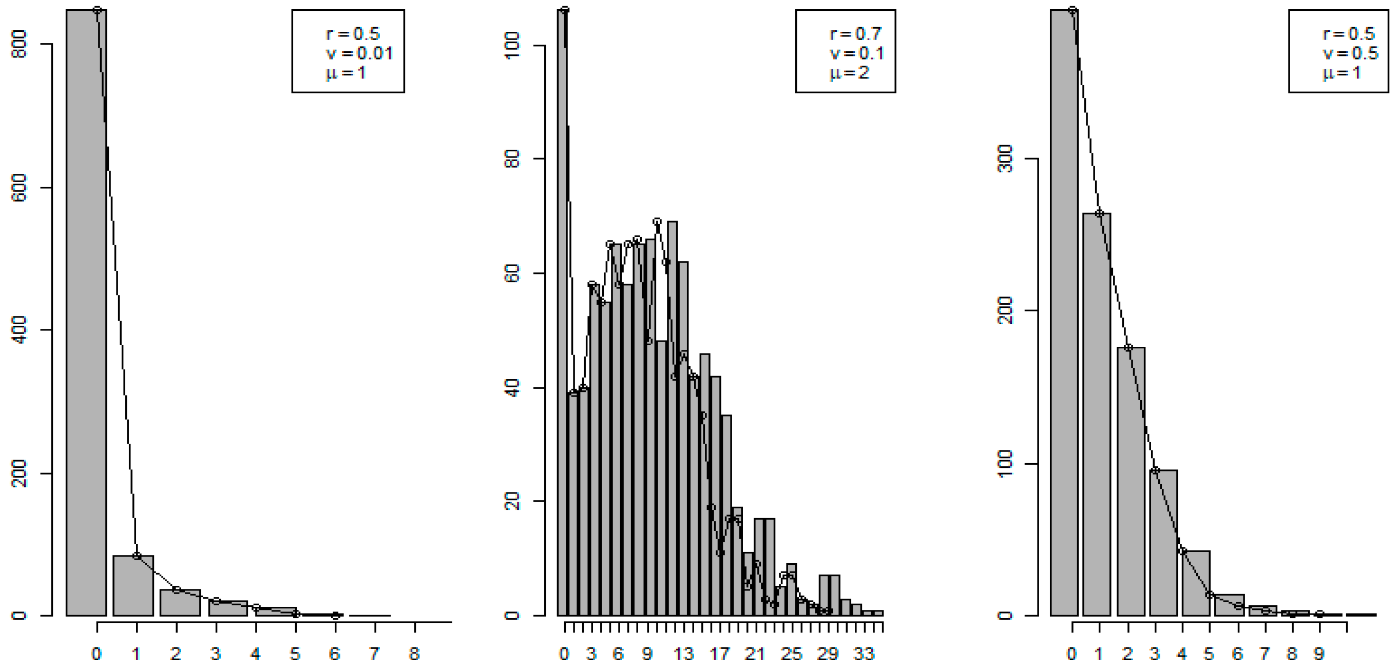
The GCOMP distribution extends the NB distribution when r equals 1. Likewise, when parameters μ ,   1 r , and ν approach 1, the GCOMP distribution simplifies to the COMP distribution, which encompasses Poisson, NB, and geometric distributions as specific cases. The range 0 < r < 1 characterizes OD, while r < 0 indicates UD in count data. Comparatively, for ν greater than 1 and 0 < r < 1 , the GCOMP distribution is more LT than the COMP distribution, whereas for ν greater than 1 and r less than 0, it demonstrates ST behavior. Figure 1 illustrates the GCOMP distribution’s behavior across parametric configurations.
The calculation of the normalizing constant is linked to the moments of the GCOMP distribution. Through the asymptotic approximation of C r , v , μ ,   valid for r < 1 , Imoto [28] has obtained the approximate formula for moments. This process yields expressions for the expected value and variance as follows:
E X = μ l o g C r , ν , μ μ μ 1 1 r + 2 ν 1 r 2 1 r ,
V a r X = μ E X μ μ 1 1 r 1 r .
The maximum likelihood estimation approach can be used to estimate parameters of the GCOMP distribution by utilizing the log likelihood function in the following manner:
l r , v , μ | X = l o g i = 0 n Γ ν + x μ x i x i ! C r , ν , μ ,
where x i   is the observed frequency of the i events. Fisher’s scoring method can be used to solve the expression presented in (5). The numerical computation of log likelihood expression in (5) could be challenging due to statistical complexities such as precision issues with extremely small or large probabilities, high dimensionality, local optima, and numerical integration.
It can be observed that the GCOMP distribution depicts the behavior of unimodal distribution when a space of (2) is set as r < 0 or r < 1 and v > 1 . The GCOMP distribution also becomes a bimodal distribution when 0 < v < 1 ,   0 < r < 1 and μ v r < 1 . One of the modes for bimodal distributions locates at zero. Because of this characteristic, the GCOMP distribution is more suited to simulate ZI count data. The ZI behavior of the GCOMP distribution is shown in Figure 2. Since it represents the ZI count data without using the ZI property, as other traditional ZI models do, the GCOMP distribution is noteworthy. The GCOMP distribution was shown to be more versatile than the COMP distribution due to its adaptability to dispersion, tail length, and significance to ZI.

2.2. Proposed G-Chart to Monitor Count Data

Assume that a univariate process at consecutive time points X 1 , X 2 , X 3 , , X n   originates n independent observations, particularly quality measurements or surveillance characteristics from the GCOMP distribution. Also, assume that these observations have standard in-control GCOMP distribution with the process mean μ 0 l o g C r , ν , μ 0 μ 0 and follow the GCOMP distribution with the shifted process mean μ 1 l o g C r , ν , μ 1 μ 1 when the process becomes out of control. Our focus lies in monitoring the stability of the total number of counts under the GCOMP distribution in this study. For this purpose, L σ control limits are obtained using the established Shewhart’s methodology [31]. Control limits are set considering G = i = 1 n X i for the total number of counts at subgroup size n. Hence, the mean and variance of statistic G are provided as:
    E G = n   μ l o g C r , ν , μ μ ;   V G = n μ E X μ
In Table 1, lower, central, and upper control limits (LCL, CL, UCL) for the proposed control chart are provided.
The control limits of the G-chart provided in Table 1 are approximately equal to the control limits of Q-chart (total number of counts chart) based on the COMP distribution proposed by Sellers [9] at μ ,   1 r and when ν 1 . Moreover, it also encompasses the Poisson distribution-based c-chart at v = 1 , and the geometric distribution-based g-chart at v = 0 and μ < 1 .

3. Findings and Discussion

In this section, the results of a thorough simulation analysis are presented to assess the performance of the proposed chart. The primary goal is to assist practitioners in monitoring UD, OD, and ZI count data by assessing the influence of the CC using the GCOMP model. Average run length (ARL), which is one of the widely used measurements, is utilized to assess the effectiveness of the proposed CC. Before initiating simulations, it is imperative to determine the values of the chart multiplier (L) associated with the control limits of any chart. Usually, practitioners prefer a value of 3 for the chart multiplier. In order to ensure that control limits yield the pre-specified false alarm probability ( α ) for any given sample size, the value of L can be chosen carefully [10]. Therefore, in this study, L control limits are determined to achieve α = 0.0027 through a Monte Carlo simulation using 10,000 iterations in R-language (version 4.1.1). The value of α = 0.0027 is selected to yield a desired observation of in-control ARL (ARL0), which is approximately equal to 370. The procedural flow chart describing the computation of CC multiplier L for the G-chart to achieve A R L 0 370 is presented in Figure 3. Corresponding values of CC multiplier L for the G-chart to obtain A R L 0 370 at different sample sizes and various parametric values are provided in Table 2. This study explored generating control limits and evaluating the performance of the proposed chart at v > 1 , which is relevant to note when examining tail behavior in UD and OD count data. The ZI in the count data is considered following the parametric setting of the GCOMP distribution mentioned in Section 2.

3.1. UD and OD Cases Considering Tail Behavior

The proposed G-chart performance is evaluated using out-of-control ARL (ARL1) profiles at different values of μ ,     r , and v . The efficacy of the proposed chart is assessed on the smaller values of ARL1, which indicate the average number of samples needed to identify out-of-control signals that are well thought out due to the fact that unusual cause μ 0 of the process may shift ( δ ) to μ 1 = μ 0 ± δ . To approximate the ARL1 profile, we again used the Monte Carlo approach and performed 10,000 iterations in R-language using sample sizes of n = { 3,15,50,100,300,1000 } simulated from the GCOMP distribution. Over-dispersed and longer-tailed (OD-LT) ( 0 < r < 1 , &   v > 1 ) as well as under-dispersed and shorter-tailed (UD-ST) ( r < 0 , &   v > 1 ) cases are considered while reporting results [32]. As per the requirement for the shifted process, shifts in the μ 0 are introduced as δ = { 0.1,0.2,0.3,0.5 } for the G-chart. The proposed G-chart is expected to perform better than the Q-chart based on the COMP distribution [10]. Therefore, the performance evaluation of the Q-chart is also conducted for comparison purposes. For a rationale comparison, the maximum likelihood estimated (MLE) values of the parameters ( μ and r) of the COMP distribution are computed for simulated data. Furthermore, the Monte Carlo simulation study is conducted to determine the values of L for the Q-chart to achieve A R L 0 370 , and then the ARL1 profiles are obtained by introducing shifts in μ 0 . In Table 3 and Table 4, the results of the ARL1 profiles for the G and Q charts, along with the values of L and valid MLEs for the Q-chart, are presented.
Table 3 shows that the G-chart performed efficiently in identifying out-of-control signals than the competitive Q-chart when the upward shift in the process is considered at different sample size n for the UD-ST model. However, the G-chart performs comparatively poorly for the downward shift compared to the Q-chart.
Table 4 shows that the G-chart performed efficiently in monitoring out-of-control signals than the Q-chart at different sample sizes n for the OD-LT model at both upward and downward shifts at most of the shifts.
The above discussion indicates that the proposed chart efficiently detects shifts in the processes when the tail behavior of the count data is considered. As expected, it is also observed in Table 3 and Table 4 that with an increase in n , the G-chart becomes more effective and sensitive in detecting out-of-control signals.

3.2. Zero-Inflation Case

Zero-inflation phenomena are observed in manufacturing, health care, and high-yield processes. The concept of zero inflation emerges frequently in the context of count data analysis. It refers to a phenomenon in which the observed data contain more zeros than a conventional count distribution would predict. Many probability distributions such as ZIP and ZINB utilize and embed ZI property to model ZI count data. The GCOMP distribution tends to model the ZI count data. It is essential to mention that the GCOMP distribution did not invoke the ZI property compared to other ZI probability distributions that model ZI data. Additionally, even though they are adept at modeling and observing ZI data, ZI models may not consistently offer a practical solution [33].
We studied the feature of the GCOMP distribution to model the ZI count data through the proposed chart and conducted a comparison with charts based on ZIP, ZINB, and ZICOMP distributions. We have simulated random samples of size n under the excessive zeros generating a parametric setting ( 0 < r < 1 ,   0 < v < 1 ) of the GCOMP distribution. The ARL1 profiles for the G-chart are obtained at n 1 = 100 ,   μ 0 = 1 ,   v = 0.05 ,   r = 0.3 (Data-I) and at n 2 = 100 , μ 0 = 1.5 ,   v = 0.1 ,   r = 0.5 (Data-II) . The ZIP, ZINB, and ZICOMP charts are modified considering the total number of counts (ZIPC, ZINBC, ZICOMPC). It is important to note that the ZIPC chart is based on the ZIP ( μ , p z i ). The ZINBC chart is based on the ZINB ( μ , r , p z i ) . And the ZICOMPC is based on the ZICOMP ( μ , r , p z i ) . The ZI parameter, p z i , in the ZIP, ZINB, and ZICOMP distributions provides the additional probability thrust to the value 0. The ARL1 profiles of the ZIPC, ZINBC, and ZICOMPC charts are computed following the MLE values of the parameters of the ZIP, ZINB, and ZICOMP distribution for Data-I and Data-II. For Data-I and Data-II, the Monte Carlo simulation study is conducted to determine the values of L for the G, ZIPC, ZINBC, and ZICOMPC charts to achieve A R L 0 370 .
Here, upward shifts ( μ 0 + δ ) are monitored in the ZI count process, where δ = { 0.1 , 0.3 , 0.5 , 0.7 , 1 } . The results of all charts for detecting shifts in the ZI count data along with values of L and the estimated parameters for the ZIPC, ZINBC, and ZICOMPC charts are reported in Table 5 and Table 6. It is evident from Table 5 and Table 6 that the GCOMP-based CC is more efficient in detecting out-of-control signals as compared to competitive CCs. Hence, this emphasizes the effectiveness of monitoring ZI data without using ZI property through the chart based on the GCOMP distribution.

4. Illustrative Examples

This section is based on the real-life and numerical applications containing some level of dispersion for the proposed G-chart.

4.1. OD-LT Count Data: Early Detection in COVID-19 Mortality Cases

In public health surveillance and healthcare monitoring, CCs are widely used [34] to help health and public authorities make vital decisions. During the ongoing COVID-19 pandemic, health authorities are keenly observing the trend of cases, mortalities, and recoveries to advise the public authorities in implementing appropriate interventions for the safety of the masses. Understanding the variation and behavior of pandemics can be facilitated by using CCs when the trend of cases and mortalities is shifting. The proposed CC was employed to monitor the counts of total number of deaths in a day due to COVID-19 in El Salvador during 8 June 2020, and 17 May 2021. The data are available on https://covid19.who.int/ (accessed on 1 August 2021) and are provided in Table 7. The data show OD with x ¯ = 6.22 and σ = 11.15 .
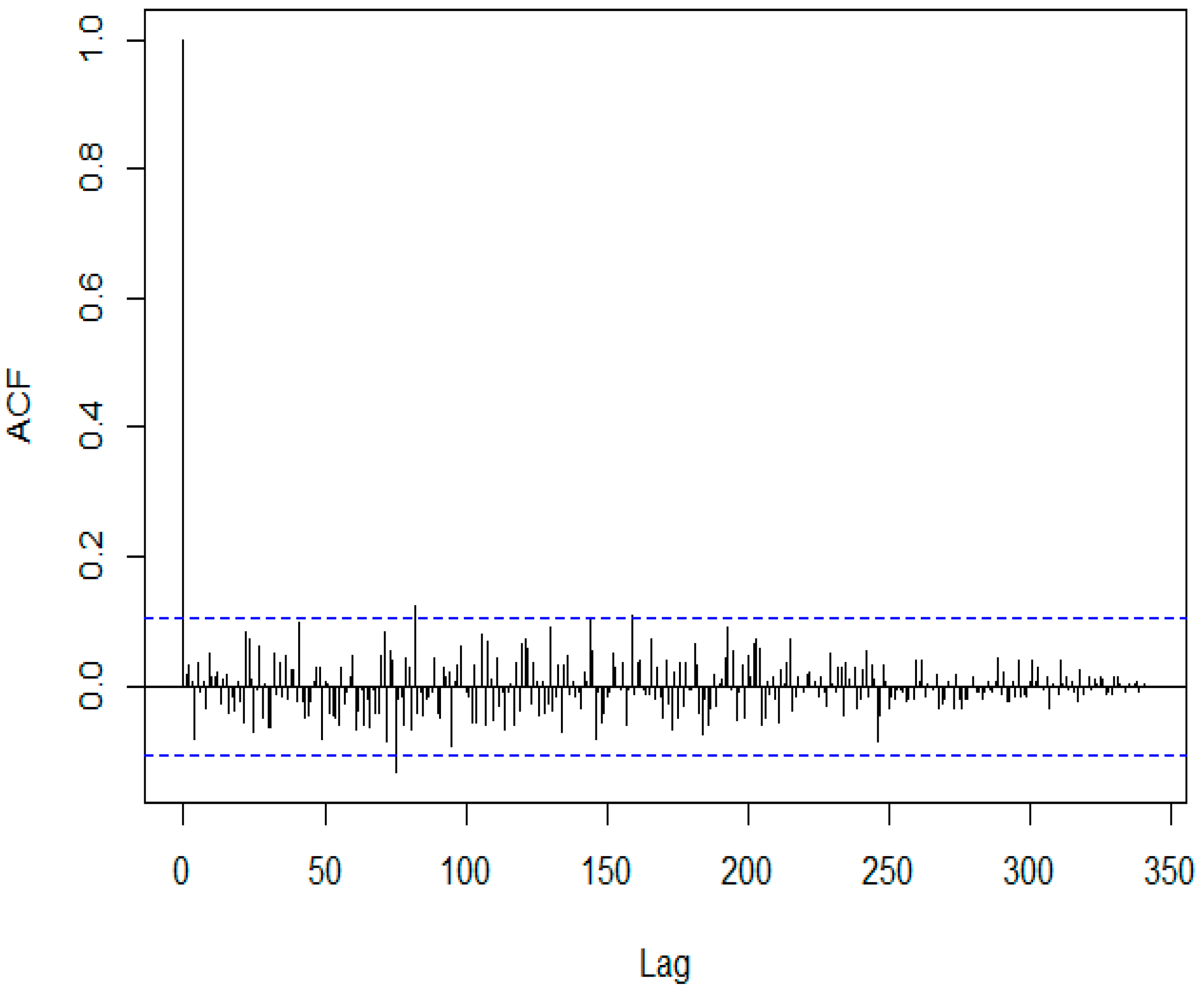
Furthermore, an assessment of serial correlation has been conducted to analyze the dependency among the occurrences of death over a given time span, a factor that is deemed unfavorable for the implementation of our suggested chart scheme. As a result, the autocorrelation function (ACF) in R-language was employed to evaluate the serial correlation of the COVID-19 death count data in El Salvador. Figure 4 presents the ACF values for the dataset with a one-day interval (lag). From the figure, it can be deduced that consecutive observations show negligible correlation, as the ACF values are close to zero, indicating minimal impact of lags.
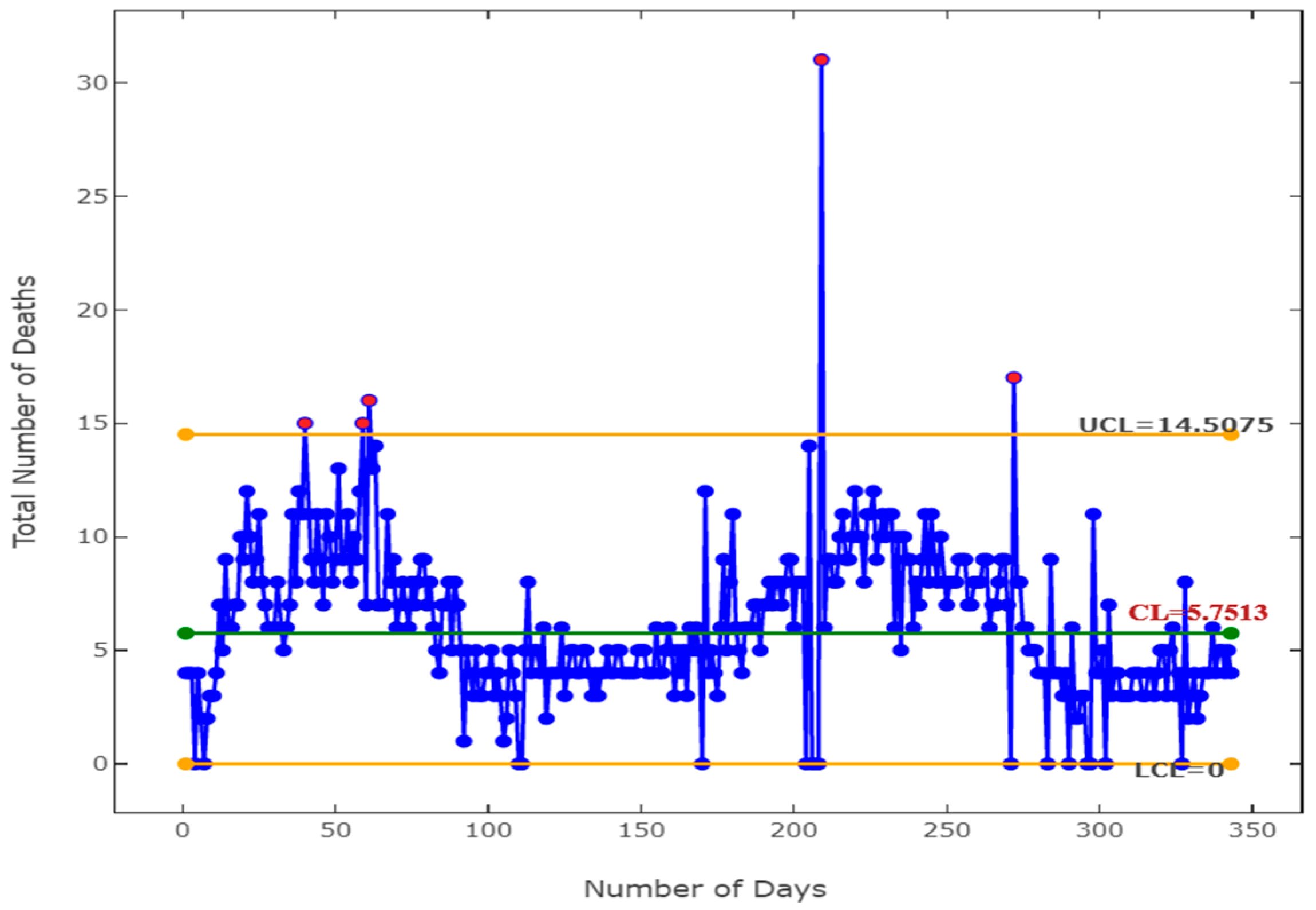
Additionally, monitoring is conducted using the existing Q-chart [10] for comparative purposes. Table 8 provides the MLEs of the model parameters for the GCOMP and COMP distribution for targeted data along with negative log likelihood (LL), Akaike Information Criterion (AIC), and Bayesian Information Criterion (BIC) for fitting and comparison purposes. Table 8 makes it clear that, in comparison to the COMP distribution, the GCOMP distribution offers a better fit for the data based on the all-criterion values. The estimated parametric values of the GCOMP distribution in Table 7 confirm that the data also exhibit longer-tail behavior ( v > 1 ). In Figure 5 and Figure 6, we presented the G-chart and Q-chart for monitoring the total number of daily deaths in El Salvador to achieve A R L 0 370 . In Table 8, the control limits for G-chart and Q-chart are set considering the parametric values mentioned. It is observed that the proposed chart trigger signals (red dots) on the 40th, 59th, 61st, 209th, and 272nd days during the phase while the competitive chart trigger signals only on the 209th and 272nd days. As expected, the proposed chart can identify process variation more quickly than the existing chart when El Salvador’s death toll begins to rise (that could turn the situation out of control). This could help the relevant authorities to take appropriate and quick action, especially during the pandemic. Consequently, it is evident that, in comparison to the existing CC, the proposed chart encourages prompt action when specific cause variation signals a new phase more quickly when the data are OD-LT.

4.2. UD-ST Count Data: A Simulated Data

The GCOMP distribution tends to model the UD count data. It is important to mention that the GCOMP distribution displays ST behavior for the parametric setting, which is calibrated to achieve UD, as discussed in previous sections. In the second application, a simulated dataset is utilized, where the total number of events are generated through the GCOMP distribution. We have simulated n 1 = 100 observations with a parametric setting of μ 0 = 1 ,   v = 1.5 , and r = 0.5 , which will be utilized for Phase-I monitoring, and then simulated n 2 = 50 observations with v = 1.5 , r = 0.5 , and μ 1 = μ 0 , where = μ 0 + 0.5 for Phase-II monitoring. Table 9 displays both of the simulated datasets.
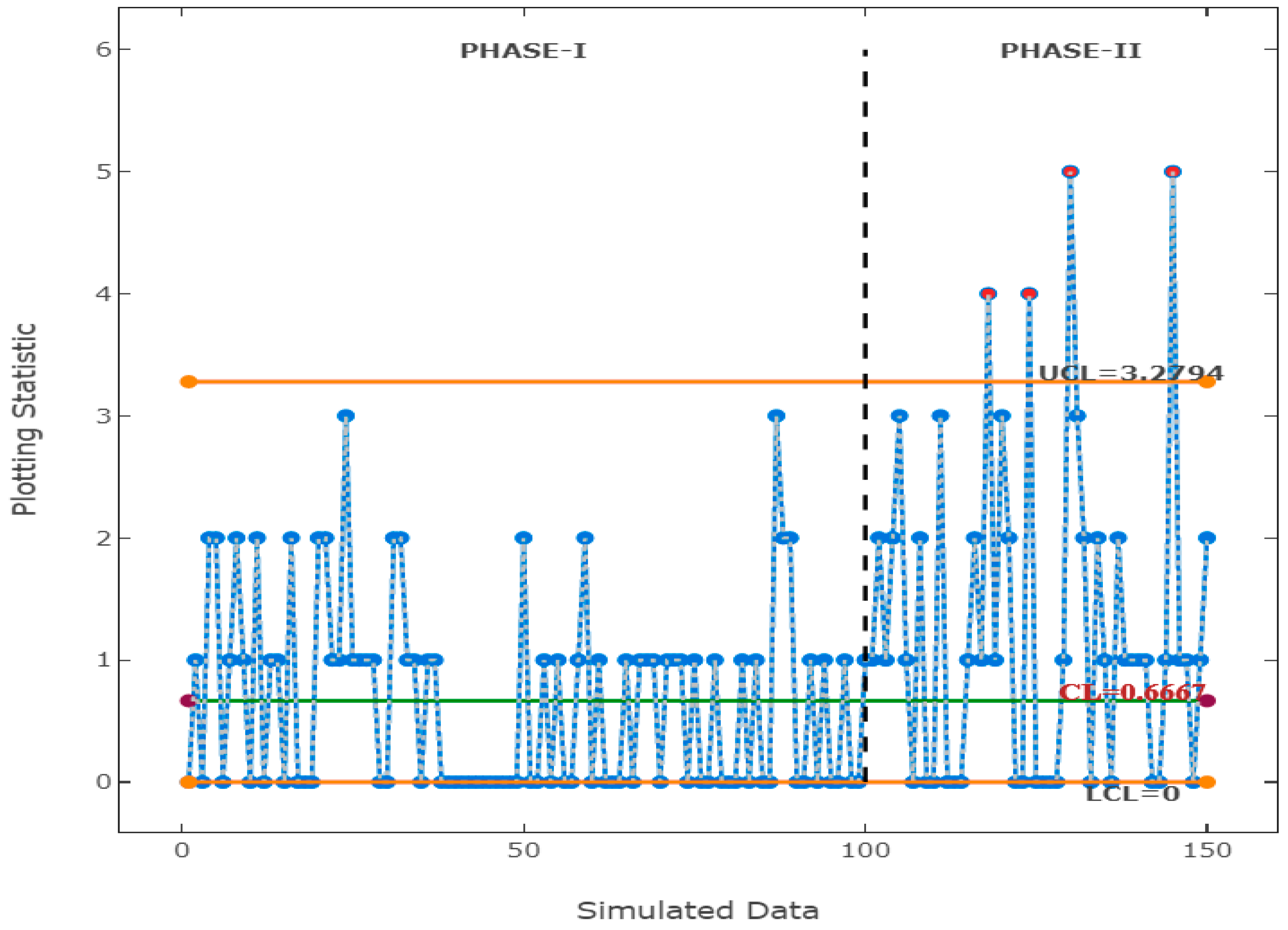
The G-chart is presented in Figure 7 for both Phase-I and Phase-II monitoring of the simulated data set (Phase-I for 1–100 observations and Phase-II for 101–150 observations, separated by dotted lines in the Figure) to yield A R L 0 370 . The control limits for G-chart are set at μ 0 = 1 ,   v = 1.5 , r = 0.5 , and L = 3.200 . When used for Phase-II monitoring, the proposed chart trigger alarms, but not for Phase-I monitoring, as would be expected.

4.3. ZI Count Data: Monitoring Number of Defective LEDs

In the third application, we consider the data set used by He et al. [35] to monitor the zero-inflation in the total number of defectives in LEDs within a batch. The dataset contains 100 observations each for Phase-I and Phase-II monitoring purposes. The datasets are accessible in Table 10. Due to some assignable causes, some values (in bold) are removed [36]. To determine if both datasets follow the GCOMP distribution, the score statistic test is utilized [37]. For this statistic, the null hypothesis yields an asymptotic χ 2 distribution with one degree of freedom. The score statistic used is:
Z = ( n z n i l o ) 2 n i l o 1 l o n i x ¯ ( l o ) 2
where n z is the total number of zero-value observations in the data; n i is the total number of observations, l o = e p ^ , in which p ^ is the estimated Poisson parameter under the null hypothesis; and x ¯ is the average of the observations. For the Phase-I dataset, n i = 96 , n z = 84 , and p ^ = x ¯ = 0.69 ; for the Phase-II dataset,   n i = 100 , n z = 79 , and p ^ = x ¯ = 1.37 . The χ 2 -value for the Phase-I dataset at 1 degree of freedom is 177.16 with a near-zero p-value; for the Phase-II dataset, it is 284.12 at 1 degree of freedom, and also with a near-zero p-value. It can be inferred that the GCOMP distribution is followed by both Phase-I and Phase-II datasets. The valid MLEs of the GCOMP distribution for the LED dataset are μ ^ 0 = 0.4679 ,   v ^ = 0.000045 , and r ^ = 2.2705 . Figure 8 shows the monitoring of the defective LED data through the G-chart to yield A R L 0 370 . The control limits for the G-chart are set at L = 3.00 and at valid MLE values of the GCOMP distribution for the LED dataset. During Phase-I monitoring, it was found that all 96 observations are in control. Our proposed chart detects a few out-of-control batches (red dots) during Phase-II monitoring.

5. Conclusive Remarks

Poisson distribution-based CCs are employed to monitor count data. However, despite their widespread usage, these CCs are not suitable for tracking UD and OD within count data because Poisson distribution relies on an equi-distribution assumption. The tail behavior of count data is also overlooked during its monitoring. In this study, a CC based on the GCOMP distribution is proposed to monitor the total number of UD, OD, and ZI counts. During monitoring, the count data’s tail behavior is taken into consideration. Both longer- and shorter-tail behaviors are anticipated. When compared to the existing CCs for the OD-LT count data, the proposed chart has been shown to be more effective at identifying both upward and downward shifts in the process. It is also noticed that proposed the CCs outperform existing CCs in detecting upward shifts for the UD-ST count data. Compared to conventional ZI models, the GCOMP distribution effectively monitors the ZI count data without utilizing the ZI property. Researchers studying this area may find great value in the GCOMP distribution’s adaptability in monitoring several critical features of the count data. Applying the Shewhart technique, researchers might investigate the GCOMP distribution’s suitability for monitoring dispersed count data while taking tail behavior into consideration for the average number of counts. Considering the variation in the count data-generating process, the feasibility of probability control limits instead of L σ control limits could also be explored for the GCOMP process. Furthermore, to improve the performance of L σ limits, the asymmetrical structure of L σ limits can also be considered in the future.

Author Contributions

Conceptualization, F.M. and R.A.K.S.; methodology, F.M., M.A.R. and R.A.K.S.; software, F.M.; validation, R.A.K.S., M.A.R. and J.A.D.; formal analysis, F.M.; investigation, M.A.R.; resources, J.A.D.; data curation, F.M.; writing—original draft preparation, F.M. and M.A.R.; writing—review and editing, M.A.R. and J.A.D.; visualization, F.M. and M.A.R.; supervision, R.A.K.S. and M.A.R. All authors have read and agreed to the published version of the manuscript.

Funding

This research received no external funding.

Data Availability Statement

The data are provided in this paper.

Conflicts of Interest

The authors declare that they have no conflicts of interest to report regarding this present study.

References

  1. Spiegelhalter, D.J. Handling over-dispersion of performance indicators. Qual. Saf. Health Care 2005, 14, 347–351. [Google Scholar] [CrossRef]
  2. Mohammed, M.A.; Laney, D. Overdispersion in health care performance data: Laney’s approach. Qual. Saf. Health Care 2006, 15, 383–384. [Google Scholar] [CrossRef] [PubMed]
  3. Albers, W. Control charts for health care monitoring under overdispersion. Metrika 2011, 74, 67–83. [Google Scholar] [CrossRef]
  4. Famoye, F. Statistical control charts for shifted generalized poisson distribution. J. Ital. Stat. Soc. 1994, 3, 339–354. [Google Scholar] [CrossRef]
  5. Fang, Y. c-charts, X-charts, and the Katz family of distributions. J. Qual. Technol. 2003, 35, 104–114. [Google Scholar] [CrossRef]
  6. He, B.; Xie, M.; Goh, T.N.; Tsui, K.L. On Control Charts Based on the Generalized Poisson Model. Qual. Technol. Quant. Manag. 2006, 3, 383–400. [Google Scholar] [CrossRef]
  7. Xie, M.; He, B.; Goh, T.N. Zero-inflated poisson model in statistical process control. Comput. Stat. Data Anal. 2001, 38, 191–201. [Google Scholar] [CrossRef]
  8. Chen, N.; Zhou, S.; Chang, T.S.; Huang, H. Attribute control charts using generalized zero-inflated poisson distribution. Qual. Reliab. Eng. Int. 2008, 24, 793–806. [Google Scholar] [CrossRef]
  9. Sellers, K.F. A generalized statistical control chart for over- or under-dispersed data. Qual. Reliab. Eng. Int. 2012, 28, 59–65. [Google Scholar] [CrossRef]
  10. Saghir, A.; Lin, Z.; Abbasi, S.A.; Ahmad, S. The use of probability limits of COM-poisson charts and their applications. Qual. Reliab. Eng. Int. 2013, 29, 759–770. [Google Scholar] [CrossRef]
  11. Saghir, A.; Lin, Z. Cumulative sum charts for monitoring the COM-Poisson processes. Comput. Ind. Eng. 2014, 68, 65–77. [Google Scholar] [CrossRef]
  12. Alevizakos, V.; Koukouvinos, C. A progressive mean control chart for COM-Poisson distribution. Commun. Stat. Part B Simul. Comput. 2020, 51, 849–867. [Google Scholar] [CrossRef]
  13. Chen, J.-H. A Double Generally Weighted Moving Average Chart for Monitoring the COM-Poisson Processes. Symmetry 2020, 12, 1014. [Google Scholar] [CrossRef]
  14. Aslam, M.; Ahmad, L.; Jun, C.H.; Arif, O.H. A Control Chart for COM–Poisson Distribution Using Multiple Dependent State Sampling. Qual. Reliab. Eng. Int. 2016, 32, 2803–2812. [Google Scholar] [CrossRef]
  15. Aslam, M.; Al-Marshadi, A.H. Design of a Control Chart Based on COM-Poisson Distribution for the Uncertainty Environment. Complexity 2019, 2019, 8178067. [Google Scholar] [CrossRef]
  16. Adeoti, O.A.; Malela-Majika, J.C.; Shongwe, S.C.; Aslam, M. A homogeneously weighted moving average control chart for Conway–Maxwell Poisson distribution. J. Appl. Stat. 2022, 49, 3090–3119. [Google Scholar] [CrossRef] [PubMed]
  17. Rao, G.S.; Aslam, M.; Rasheed, U.; Jun, C.-H. Mixed EWMA–CUSUM chart for COM-Poisson distribution. J. Stat. Manag. Syst. 2020, 23, 511–527. [Google Scholar] [CrossRef]
  18. Rakitzis, A.C.; Maravelakis, P.E.; Castagliola, P. CUSUM Control Charts for the Monitoring of Zero-inflated Binomial Processes. Qual. Reliab. Eng. Int. 2016, 32, 465–483. [Google Scholar] [CrossRef]
  19. Ho, L.L.; Andrade, B.; Bourguignon, M.; Fernandes, F.H. Monitoring count data with Shewhart control charts based on the Touchard model. Qual. Reliab. Eng. Int. 2021, 37, 1875–1893. [Google Scholar] [CrossRef]
  20. Bourguignon, M.; Medeiros, R.M.R.; Fernandes, F.H.; Lee Ho, L. Simple and useful statistical control charts for monitoring count data. Qual. Reliab. Eng. Int. 2021, 37, 541–566. [Google Scholar] [CrossRef]
  21. Boaventura, L.L.; Ferreira, P.H.; Fiaccone, R.L. New statistical process control charts for overdispersed count data based on the Bell distribution. An. Acad. Bras. Ciências 2023, 95, e20200246. [Google Scholar] [CrossRef]
  22. Raza, M.A.; Aslam, M. Design of control charts for multivariate Poisson distribution using generalized multiple dependent state sampling. Qual. Technol. Quant. Manag. 2019, 16, 629–650. [Google Scholar] [CrossRef]
  23. Aslam, M.; Saghir, A.; Ahmad, L.; Jun, C.H.; Hussain, J. A control chart for COM-Poisson distribution using a modified EWMA statistic. J. Stat. Comput. Simul. 2017, 87, 3491–3502. [Google Scholar] [CrossRef]
  24. Urbieta, P.; Lee, H.O.L.; Alencar, A. CUSUM and EWMA Control Charts for Negative Binomial Distribution. Qual. Reliab. Eng. Int. 2017, 33, 793–801. [Google Scholar] [CrossRef]
  25. Alevizakos, V.; Koukouvinos, C. Monitoring of zero-inflated binomial processes with a DEWMA control chart. J. Appl. Stat. 2021, 48, 1319–1338. [Google Scholar] [CrossRef] [PubMed]
  26. Mustafa, F.; Sherwani, R.A.K.; Raza, M.A. A new exponentially weighted moving average control chart to monitor count data with applications in healthcare and manufacturing. J. Stat. Comput. Simul. 2023, 93, 3308–3328. [Google Scholar] [CrossRef]
  27. Mustafa, F.; Sherwani, R.A.K.; Raza, M.A. On designing a cumulative sum control chart using generalized Conway-Maxwell-Poisson distribution for monitoring the count data. Eur. J. Ind. Eng. 2024, 18, 637–668. [Google Scholar] [CrossRef]
  28. Imoto, T. A generalized Conway-Maxwell-Poisson distribution which includes the negative binomial distribution. Appl. Math. Comput. 2014, 247, 824–834. [Google Scholar] [CrossRef]
  29. Saghir, A.; Lin, Z. A flexible and generalized exponentially weighted moving average control chart for count data. Qual. Reliab. Eng. Int. 2014, 30, 1427–1443. [Google Scholar] [CrossRef]
  30. Sellers, K.F.; Shmueli, G. A flexible regression model for count data. Ann. Appl. Stat. 2010, 4, 943–961. [Google Scholar] [CrossRef]
  31. Montgomery, D.C. Introduction to Statistical Quality Control; Wiley: Hoboken, NJ, USA, 2013. [Google Scholar]
  32. Mustafa, F.; Khan Sherwani, R.A.; Raza, M.A. A progressive mean control chart for dispersed count data considering tail behavior. Qual. Technol. Quant. Manag. 2023, 1–20. [Google Scholar] [CrossRef]
  33. Campbell, H. The consequences of checking for zero-inflation and overdispersion in the analysis of count data. Methods Ecol. Evol. 2021, 12, 665–680. [Google Scholar] [CrossRef]
  34. Woodall, W.H. The use of control charts in health-care and public-health surveillance. J. Qual. Technol. 2006, 38, 89–104. [Google Scholar] [CrossRef]
  35. He, S.; Huang, W.; Woodall, W.H. CUSUM charts for monitoring a zero-inflated poisson process. Qual. Reliab. Eng. Int. 2012, 28, 181–192. [Google Scholar] [CrossRef]
  36. Alevizakos, V.; Koukouvinos, C. Monitoring of zero-inflated Poisson processes with EWMA and DEWMA control charts. Qual. Reliab. Eng. Int. 2020, 36, 88–111. [Google Scholar] [CrossRef]
  37. Van den Broek, J. A score test for zero inflation in a Poisson distribution. Biometrics 1995, 51, 738–743. [Google Scholar] [CrossRef]
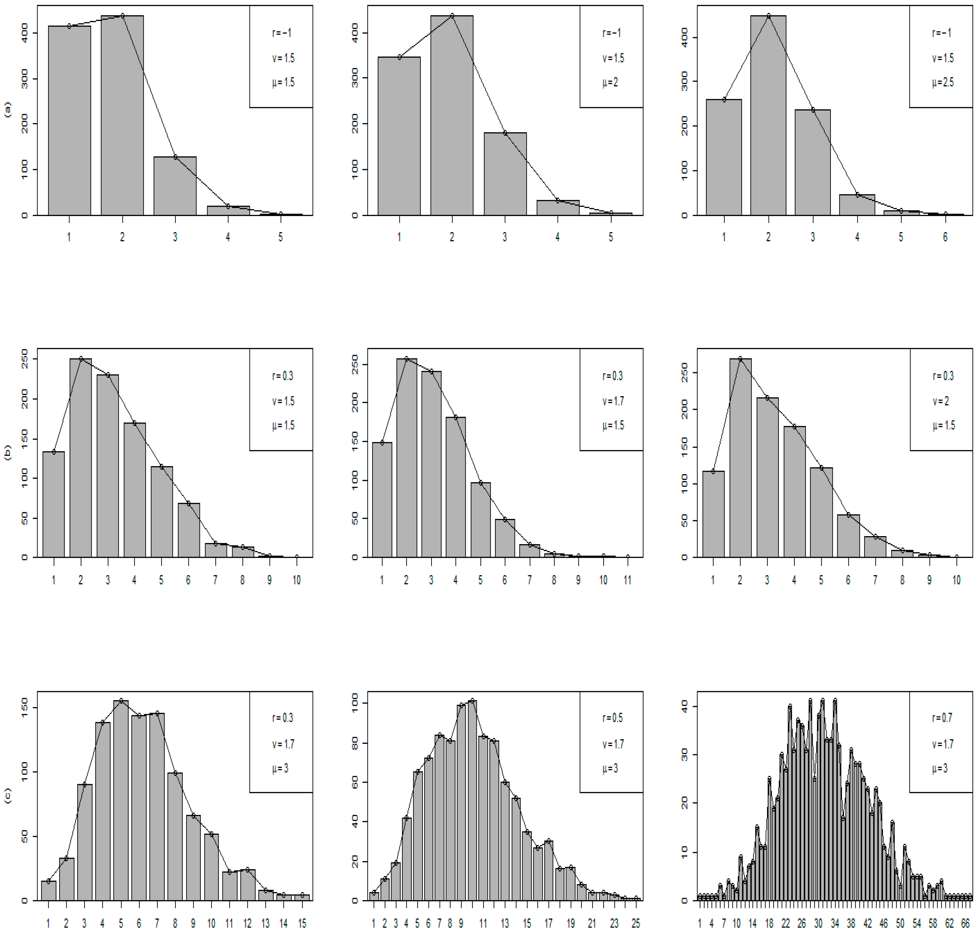
Figure 1. Behavior of GCOMP distribution at different parametric settings. Panel (a) depicts under-dispersed and shorter-tail behavior of the GCOMP distribution at different parametric values, and Panel (b,c) depicts over-dispersed and longer-tail behavior of the GCOMP distribution at different parametric values.
Processes 12 00688 g001
Figure 2. ZI behavior of the GCOMP distribution at different parametric values.
Processes 12 00688 g002
Figure 3. Flow chart for computation of CC multiplier L for G-chart to achieve A R L 0 370 .
Processes 12 00688 g003
Figure 4. ACF plot for El Salvador COVID-19 mortality data.
Processes 12 00688 g004
Figure 5. Monitoring the total number of daily deaths due to COVID-19 in El Salvador through the G-chart.
Processes 12 00688 g005
Figure 6. Monitoring the total number of daily deaths due to COVID-19 in El Salvador through the Q-chart.
Processes 12 00688 g006
Figure 7. Phase-I and Phase-II monitoring of UD-ST count data through the G-chart.
Processes 12 00688 g007
Figure 8. Phase-I and Phase-II monitoring of the total number of defective LEDs produced within a batch through the G-chart.
Processes 12 00688 g008
Table 1. Control limits for G-Chart.
G-Chart
LCL n   μ l o g C r , ν , μ μ L   n μ E X μ
CL n   μ l o g C r , ν , μ μ
UCL n   μ l o g C r , ν , μ μ + L   n μ E X μ
Table 2. L-coefficient values to achieve A R L 0 370 for G-chart.
n
r v μ 315501003001000
−0.51.513.5103.1563.1203.2003.4404.005
−0.5323.2563.6934.465.2617.07310.69
−1.51.512.8002.8613.0633.1443.3033.967
−1223.4013.3713.5214.0024.9036.751
0.322.53.0102.953.0503.1003.3023.708
0.31.513.2453.1243.2483.5514.0905.250
0.51.513.3663.4684.0994.6676.1008.550
0.5222.9653.0673.2513.5534.1055.202
0.7223.1013.0533.1803.3423.7964.622
Table 3. ARL1 profile of G-chart and Q-chart for the total sum of UD-ST count data.
ARL1
n 315501003001000
δ G-Chart
μ = 1
v = 1.5
r = 1.5
L = 2.80
Q-Chart
μ = 0.746
r = 2.100
L = 2.85
G-Chart
μ = 1
v = 1.5
r = 1.5
L = 2.86
Q-Chart
μ = 0.74
r = 2.10
L = 2.87
G-Chart
μ = 1
v = 1.5
r = 1.5
L = 3.06
Q-Chart
μ = 0.74
r = 2.10
L = 3.51
G-Chart
μ = 1
v = 1.5
r = 1.5
L = 3.14
Q-Chart
μ = 0.74
r = 2.10
L = 3.60
G-Chart
μ = 1
v = 1.5
r = 1.5
L = 3.30
Q-Chart
μ = 0.74
r = 2.10
L = 4.38
G-Chart
μ = 1
v = 1.5
r = 1.5
L = 3.96
Q-Chart
μ = 0.74
r = 2.10
L = 5.74
−0.53350.19599.019990.126.4525.91.084.111111
−0.31001.66186.23646848.744234.0191.31.7211.11.201.81
−0.2731.73000.103008.7136.36162013.91617.25.58184.01.9859.41
−0.1481.31250.181209.8344.841389.661.991853.235.764481.89.728021.72.17
0.1213.3374.25219.4256.01101.12601.8964.72201.8923.56789.15.99999
0.2156.2236.1296.5105.3439.7180.3319.1267.234.7520.131.31717.35
0.3117.3162.834754.841846.557.641.231.929.131.05.12
0.571.884.5511.117.685.59.672.351.011.5611.01
Table 4. ARL1 profile of G-chart and Q-chart for the total sum of OD-LT count data.
ARL1
n 315501003001000
δ G-Chart
μ = 1
v = 1.5
r = 0.5
L = 3.36
Q-Chart
μ = 1.41
r = 0.60
L = 3.36
G-Chart
μ = 1
v = 1.5
r = 0.5
L = 3.46
Q-Chart
μ = 1.41
r = 0.60
L = 3.10
G-Chart
μ = 1
v = 1.5
r = 0.5
L = 4.09
Q-Chart
μ = 1.41
r = 0.60
L = 3.14
G-Chart
μ = 1
v = 1.5
r = 0.5
L = 4.66
Q-Chart
μ = 1.41
r = 0.60
L = 3.16
G-Chart
μ = 1
v = 1.5
r = 0.5
L = 6.10
Q-Chart
μ = 1.41
r = 0.60
L = 3.23
G-Chart
μ = 1
v = 1.5
r = 0.5
L = 8.55
Q-Chart
μ = 1.41
r = 0.60
L = 3.56
−0.59900.129653.21.7122.8412.0111.011111
−0.36998.375023.217.64193.081.491.033.6911.0111
−0.24134.812468.2322.24758.313.6539.231.611.231.01211.01
−0.11256.881052.7184.791065.2322.13314.2310.75123.232.2529.11.016.23
0.1155.13220.4198.2388.4337.1135.3619.8920.8756.2323.23
0.268.55112.4432.6327.328.776.763.914.811.011.9911.01
0.333.1559.6910.5512.133.121.091.5211.0111
0.510.3423.232.414.121.071.19111111
Table 5. ARL1 profiles of G, ZIPC, and ZINBC CCs for Data-I.
G-ChartZIPC-ChartZINBC-ChartZICOMPC-Chart
δ μ 0 = 1 ,
v = 0.05 ,
r = 0.3
L = 2.280
μ ^ 0 = 1.39 ,
P z i = 0.71 ,
L = 4.305
μ ^ 0 = 1.17 ,
r ^ = 0.37 ,
P z i = 0.76 ,
L = 5.310
μ ^ 0 = 1.09 ,
r ^ = 0.72 ,
  P z i = 0.41 ,
L = 3.7378
0.13.2150.994.95144.66
0.31.365.452.1756.90
0.512.031.5525.37
0.711.081.0114.35
11117.24
Table 6. ARL1 profiles of G, ZIPC, and ZINBC CCs for Data-II.
G-ChartZIPC-ChartZINBC-ChartZICOMPC-Chart
δ μ 0 = 1.5 ,
v = 0.1 ,
r = 0.5 ,
L = 3.270
μ ^ 0 = 1.91 ,
P z i = 0.63
L = 8.830
μ ^ 0 = 1.67 ,
r ^ = 0.61 ,
P z i = 0.65
L = 6.450
μ ^ 0 = 1.62 ,
r ^ = 0.58 ,
  P z i = 0.35,
L = 3.501
0.123.3324.2129.63194.56
0.31.752.812.0164.91
0.51.011.841.7126.99
0.711.091.0313.50
11116.34
Table 7. Counts of total number of deaths in a day due to COVID-19 in El Salvador from 8 June 2020 to 17 May 2021.
3,4,4,4,0,4,2,0,2,3,3,4,7,5,9,6,6,7,7,10,9,12,10,8,9,11,8,7,6,6,6,8,6,5,6,7,11,8,12,11,15,11,9,8,11,9,7,11,10,8,9,13,9,9,11,8,10,9,12,15,7,16,13,14,7,7,7,11,8,9,6,7,8,7,6,8,7,8,9,9,7,8,6,5,4,7,7,8,5,8,7,5,1,5,4,3,5,3,3,4,4,5,3,4,3,1,2,5,4,3,0,0,5,8,4,5,5,4,6,2,4,4,4,4,6,3,4,5,5,4,4,5,5,4,3,4,3,4,4,5,4,4,5,5,4,4,4,4,4,5,5,5,4,4,4,6,4,4,5,6,5,3,5,4,5,3,6,5,6,5,0,12,4,5,4,3,6,9,5,8,11,6,5,4,6,6,6,7,7,5,7,7,8,7,8,8,7,8,9,9,6,8,8,8,0,14,0,0,0,31,6,9,9,8,8,10,11,9,9,10,12,10,10,8,11,11,12,9,10,11,10,11,11,6,10,5,10,9,9,6,8,7,9,11,8,11,9,8,10,8,7,8,8,8,9,9,9,7,7,8,8,9,9,6,7,7,8,9,9,7,0,17,8,8,6,6,5,5,5,4,4,4,0,9,4,4,4,3,4,0,6,2,2,3,3,0,0,11,4,4,5,0,7,3,4,4,3,3,3,3,4,4,4,3,3,4,4,3,4,5,5,3,5,6,3,4,0,8,2,3,4,2,3,4,4,4,6,4,5,5,4,5,4
Table 8. Estimated values of parameters, χ 2 , LL, AIC, and BIC for the GCOMP and COMP distribution.
ParametersCriterion
Distribution(s) μ ^ r ^ v ^ χ 2 -LLAICBIC
GCOMP2.73630.38951.3528495.43−880.9791767.9591779.472
COMP2.46360.5156 566.65−885.9791774.1891781.865
Table 9. Simulated data under the UD-ST parametric setting of the GCOMP distribution.
Phase-I DataPhase-II Data
0,1,0,2,2,0,1,2,1,0,2,0,1,1,0,2,0,0,0,2,2,1,1,3,1,1,1,1,0,0,2,2,1,1,0,1,1,0,0,0,0,0,0,0,0,0,0,0,0,2,0,0,1,0,1,0,0,1,2,0,1,0,0,0,1,0,1,1,1,0,1,1,1,0,1,0,0,1, 0,0,0,1,0,1,0,0,3,2,2,0,0,1,0,1,0,0,1,0,0,11,0,1,0,0,1,2,0,1,0,0,0,1,0,1,1,1,0,1,2,1,2,3,1,0,2,0,0,3,0,0,0,1,2,1,4,1,3,2,0,0,4,0,0,0,0,1,5,3,2,0,2,1,0,2,1,1,1,1,0,0,1,5,1,1,0,1,2
Table 10. Number of defective LEDs within a batch.
Phase-I DataPhase-II Data
0,0,19,0,0,0,0,5,0,0,0,6,0,2,0,0,0,0,0,0,0,0,0,0,0,0,0,0,0,12,0,9,0,0,0,8,0,0,0,16,0,0,0,6,3,0,0,0,0,0,0,0,0,2,0,0,0,7,0,0,0,0,0,0,0,0,0,0,0,0,0,0,0,0,0,0,0,0,0,0,8,0,0,0,18,9,0,0,0,0,2,0,0,0,0,0,0,0,0,00,0,0,19,0,0,0,0,5,0,0,6,0,2,0,0,0,0,0,0,0,0,0,0,0,0,0,0,0,12,0,10,0,0,0,8,0,0,0,0,0,16,0,6,3,0,0,0,0,0,0,0,0,0,0,0,0,0,0,5,0,2,0,8,4,0,0,0,0,0,0,0,0,0,0,1,4,0,0,6,0,2,0,9,0,0,0,0,0,0,0,0,5,0,0,0,0,4,0,0
Disclaimer/Publisher’s Note: The statements, opinions and data contained in all publications are solely those of the individual author(s) and contributor(s) and not of MDPI and/or the editor(s). MDPI and/or the editor(s) disclaim responsibility for any injury to people or property resulting from any ideas, methods, instructions or products referred to in the content.