Article

Distributed Fiber Optic Vibration Signal Logging Well Production Fluid Profile Interpretation Method Research

1
Key Laboratory of Oil and Gas Resources and Exploration Technology of Ministry of Education, Yangtze University, Wuhan 430100, China
2
PetroChina Qinghai Oilfield Company, Dunhuang 736202, China
3
PetroChina Tarim Oilfield Company, Korla 841000, China
4
Sinopec Shengli Oilfield Company, Dongying 257100, China
*
Author to whom correspondence should be addressed.
Processes 2024, 12(4), 721; https://doi.org/10.3390/pr12040721
Submission received: 17 February 2024 / Revised: 24 March 2024 / Accepted: 28 March 2024 / Published: 2 April 2024
(This article belongs to the Special Issue Application of Chemical Smart Manufacturing in Industry 4.0)

Abstract

:
Traditional logging methods need a lot of data support such as suction profile information, reservoir geological information, and production information of injection and extraction wells to calculate oil and gas production, which is a tedious and complicated process with low interpretation accuracy. Distributed fiber optic vibration signal logging is a technology that uses fiber optics to sense the vibration signals returned from different formations or well walls to analyze the surrounding formation characteristics or downhole events, which has the advantages of strong real-time monitoring results and high reliability of interpretation results. However, the currently distributed fiber optic vibration signal logging also fails to fully utilize the technical advantages to form a systematic production calculation process. Therefore, this paper proposes to use the K-means++ algorithm to divide the vibration signal frequency bands to represent different downhole events and use the amplitude mean curve envelope area of the reservoir-related frequency bands to calculate the relative production of each production formation. The experimental results correspond well with the relative water absorption data interpreted by conventional production logging, and the accuracy of production interpretation is high, which fills the gap of a production calculation method in the field of distributed fiber optic vibration signal logging in China and strongly promotes the development of the intelligent construction of oil and gas fields.

1. Introduction

An important way to monitor the dynamics of oil and gas field development is to measure the fluid flow profiles in oil recovery wells and water injection wells. The purpose of the measurement is to understand the nature and flow rate of the produced or inhaled fluid in the production well section and to make an evaluation of the production status of the well and the production properties of the formation [1,2,3,4,5]. However, in the actual oil and gas field development process, although one can know the total amount of produced oil, gas, and water, it is difficult to determine the contribution of each shot hole section stratification to the output [6]. The study of the contribution of each injection section stratification to the production capacity of the whole well and the clarification of the oil and water production location can facilitate subsequent work, such as dissection and water plugging, and can effectively improve the recovery rate of oil and gas reservoirs.
Distributed fiber optic sensing technology is an important part of the fiber optic sensing field, which can continuously sense the spatial distribution and change information of physical quantities such as temperature, strain, vibration, and so on at each point on the fiber optic transmission path. Distributed fiber optic sensing technology is increasingly used in a variety of industries [7]. For example, Sekip Esat Hayber et al. proposed a highly sensitive fiber optic microphone (FOM) based on a cellulose triacetate diaphragm in 2018. Based on the evaluation of the obtained results, the FOM can be used for medical spectral analysis and imaging applications as well as long-distance listening and speech recognition in military and public safety [8]. Moreover, Serkan Keser et al. developed a metallic hemispherical nozzle sensor based on a Fabry–Perot interferometer for surface roughness identification in 2021 [9]. In 2019, Liu Junrong et al. filtered the noise signals and derived the fractured layer segments by analyzing the area ratio and the area variance of the area bounded by the vibration energy and the minimum vibration energy of the segments in the acoustic waterfall map at a certain moment, the post-fracturing fluid-producing layer segments, and the proppant distribution [10]. In 2023, Arnaldo Leal-Junior et al. introduced a new type of fiber optic sensor system, which utilized the data fusion method of different fiber optic sensors for salinity monitoring [11]. In 2023, Lin Qingjin et al. successfully used distributed fiber optic logging technology to solve the problem of insufficient recording of dynamic monitoring data due to asphaltene precipitation during gas injection and development in the Tarim Donghe Oilfield [12]. In recent years, the software and hardware of distributed fiber optic technology have developed rapidly, but less research has been performed in the field of processing and interpreting the recorded data of distributed fiber optic vibration signals, which needs to be improved urgently.
Distributed fiber optic vibration signal logging is a technique that uses fiber optics to sense vibration signals returned from different formations or well walls throughout the transmission path for formation characterization and downhole event analysis [13,14,15,16]. This technology not only provides real-time continuous downhole information but also allows static testing with less interference to well production, easy access to the well, and is competent for small-size tubular columns. It also has a lower cost. Currently, with its rapid development, distributed fiber optic monitoring technology provides new ideas for determining output formation, accurately obtaining the output profile of oil and gas wells, and estimating fluid production.

2. Principle and Method

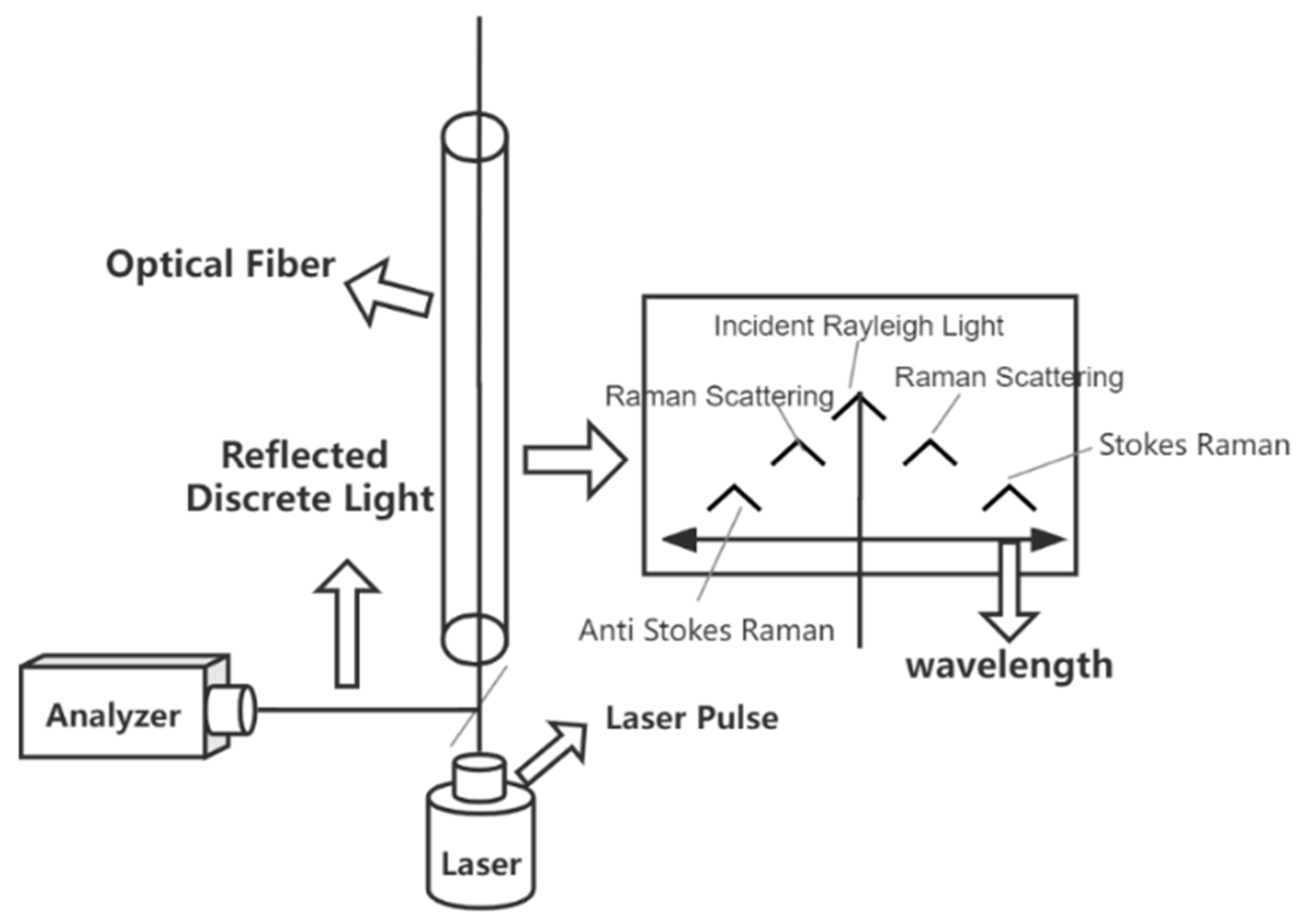
2.1. Principle of Distributed Fiber Optic Vibration Sensing System

The fiber optic sensor is mainly composed of five parts: a light source, an incident fiber, an outgoing fiber, a light modulator, a light detector, and a demodulator [17]. The principle of the distributed fiber optic vibration monitoring system is shown in Figure 1 [18].
At t = 0 , a narrow linewidth single-frequency pulsed light of angular frequency f and pulse width W is incident into the sensing fiber, and the wave function y t of the returned Rayleigh scattered light in the absence of perturbation is [19]
y t = k = 1 N cos 2 π f t τ k a k e α c τ k n k rect t τ k W  
In the above equation, N denotes the number of scattering points, τ k is the optical echo time of the k th scattering point, and a k is the amplitude [20].
rect t τ k W = 1 ,   0 t τ k W 1 0 ,   else
The above equation is the pulse width equation and the distance, Z k , between the k th scattering point and the incident end of the pulse light is [21,22]
z k = c τ k 2 n k
Then, the power of the backward Rayleigh scattered light p(t) is [23,24,25]
p t = y t 2 = p 1 t + p 2 t
p 1 t = i = 1 N a i 2 e 2 α C τ i n i rect t τ i W  
p 2 t = 2 i = 1 N 1 j = i + 1 N a i a j cos ϕ i j e α C ( τ i + τ j ) n i rect t τ i W rect t τ j W  
From Equations (1)–(4), it can be seen that the backward Rayleigh scattered optical power consists of two parts: the backward Rayleigh scattered optical power accumulated by N scattering points, p 1 t , which represents the optical power scattered by the optical signal interacting with the microstructure of the fiber material during the transmission process [26,27], and the other part of the power of different scattering points interfering with each other, p 2 t , which represents the interference effect between the different scattering points of the optical signal during the transmission process [28,29]. ϕ i j is the relative phase difference between the i-th and j-th scattering points, which can be further expressed by combining Equations (1)–(3) as
ϕ i j = 2 π f τ i τ j = 4 n π f z j z i c
From Equations (1)–(6) and (1)–(7), the interference term p 2 t is a function of f, n i and the distance z j z i from the adjacent scattering point. When vibration occurs at any position on the sensing fiber, the length and refractive index, n i , of the fiber at that point will change, causing phase modulation [10,30,31,32,33,34]. This phase modulation effect causes a corresponding change in the intensity of the backward Rayleigh scattered light, so the change in the light intensity can be detected to determine whether the vibration is occurring on the fiber and its location.

2.2. K-Means++ Algorithm

The K-means++ algorithm is a method that optimizes the randomness of the initialized centroid selection of the K-means algorithm [35,36]. Its goal is to divide the samples in the dataset into k clusters, each of which contains some similar samples. The core idea of the algorithm is to select the next center of mass by calculating the distance of the sample points from the selected center of mass so that each center of mass maximizes the distance from the other centers of mass and all the samples in the cluster.
The optimization strategy for the K-means++ initialization of the clustering centers is specified as follows:
  • Select the first cluster center, u 1 , arbitrarily and randomly among the data points as the initial cluster center.
  • For each data point X i that has not yet been selected, calculate the distance between X i and the nearest center that has been selected: D X i = arg min X i u r 2 2 , r = 1,2 , k s e l e c t e d .
  • The similarity between the data points is calculated based on the distance between them and the nearest centroid, and the probability of each data point being a new centroid is assigned proportionally. Then, a new data point is randomly selected as a new centroid from this probability distribution, where the probability of point X i being selected is proportional to D X i .
  • Repeat steps 2 and 3 until k centroids are selected.
  • For the other data points, X i , mark them as the closest classification cluster to the category center, u j .
  • Update the centroid of each category, u j , to the mean of all the samples belonging to that category.

3. Distributed Fiber Optic Vibration Signal Logging Data Processing and Interpretation Method

In the actual distributed fiber optic vibration signal logging fluid-producing profile processing, it is usually assumed that the friction signal within the rock particles and the output fluid is a minimum-phase subwave, and the friction signals generated by different pores change with the radius of the pore roar, i.e., the resulting subwave waveforms (amplitude and bandwidth) are different. On-site DAS injection profile monitoring is recorded multiple times, generally reflecting one DAS time series in five-minute monitoring steps. These data are preprocessed to obtain spectrograms. The spectrogram can be fed back once per monitoring, and the duration of a single monitoring only needs to satisfy the sampling theorem. The data preprocessing includes the time–frequency domain conversion of the distributed fiber vibration signals using the short-time Fourier transform, the thinning of the distributed fiber vibration signal data using the Douglas-Puke algorithm, and the decomposition and reconstruction of the distributed fiber vibration signals using the ARO-VMD-SSA algorithm to achieve denoising [37].

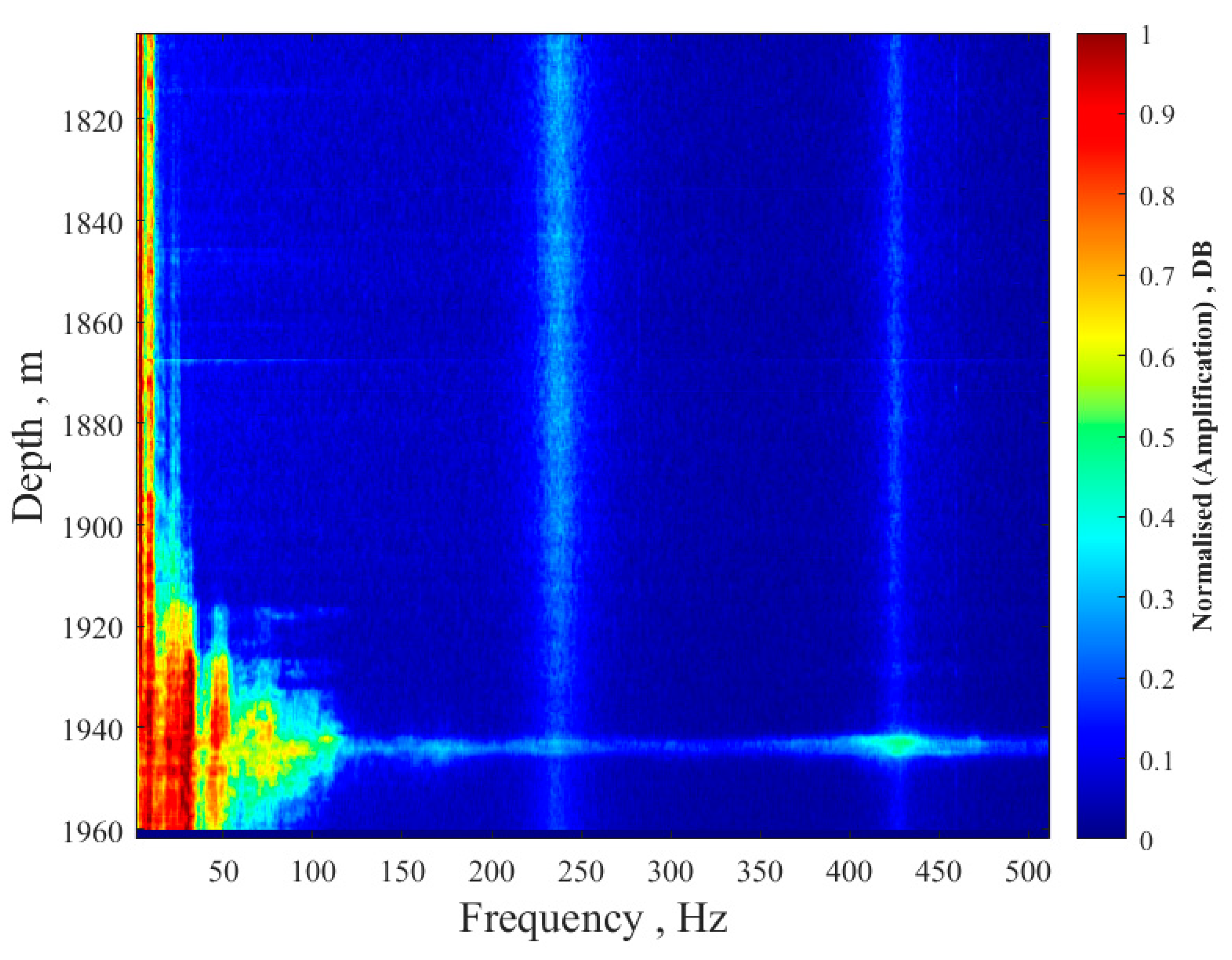
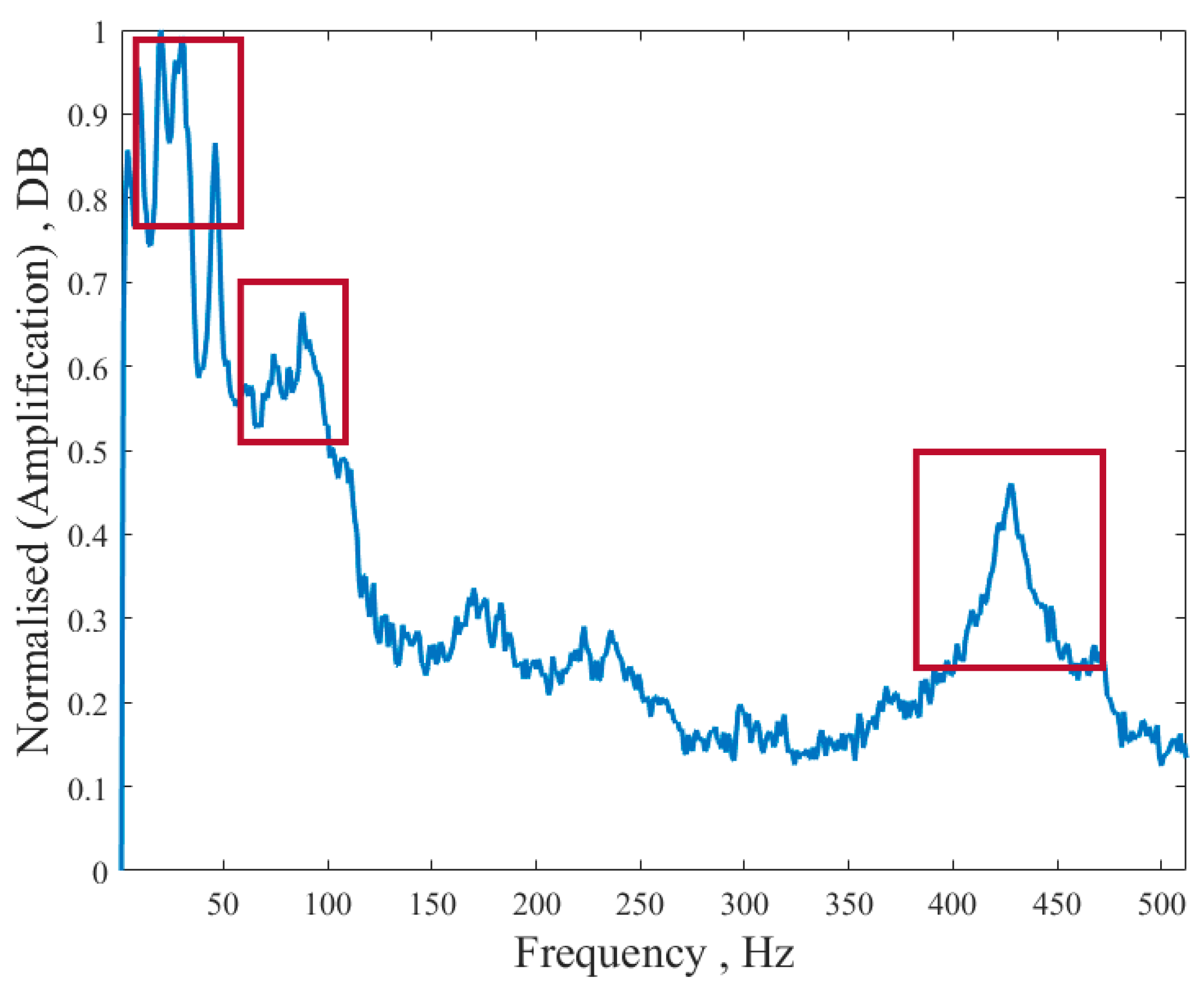
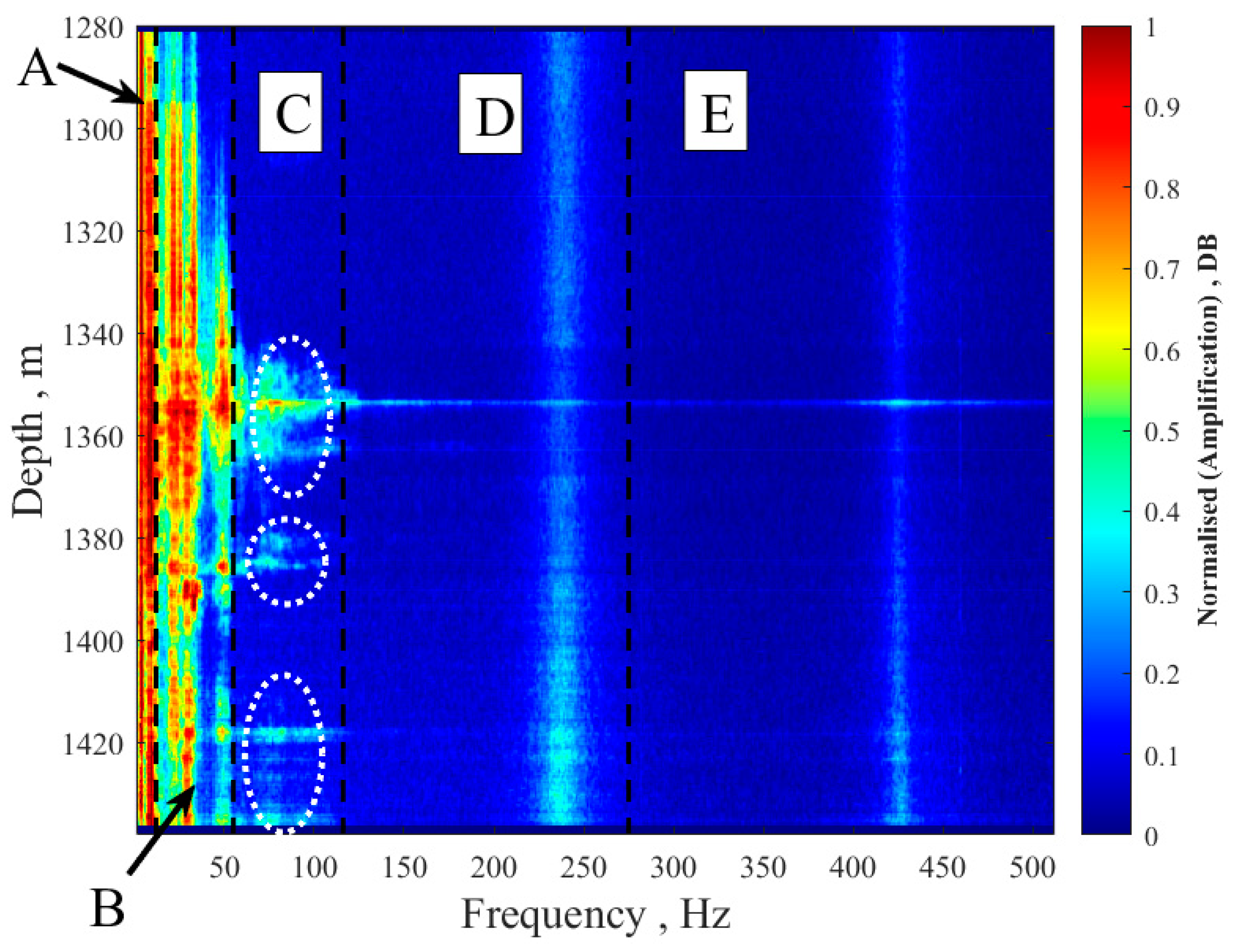
3.1. Spectrogram Analysis

The distributed fiber optic vibration signal data extracted from the fiber optic sensor for injection well A were selected for processing, and the well was logged for the purpose of detecting the extra-tubular tampering channel and the main suction layer level. The drilling depth of well A is 1993 m, the inner diameter of the casing is 139.7 mm, the inner diameter of the tubing is 62 mm, the shot hole sections are all sandstone reservoirs, and the measurement well section is 0–1961.95 m. The measurement time is from 21:23:15 on 10 May 2022 to 20:51:55 on 11 May 2022, and the frequency domain of the measurement is 0–512 Hz. The distributed fiber optic vibration signal into a spectrogram is shown in Figure 2.
The spectrum shows that the high energy points are mainly concentrated in the depth section 1913–1961 m, and there are high energy points from low frequency to high frequency at a depth of 1943 m. Therefore, it is inferred that a depth of 1943 m is the main water absorption level, and there is a situation of extraneous channeling at this location.
The analysis of the vibration signal profile for the distributed fiber at a depth of 1943 m is shown in Figure 3. Due to the large value of the measured amplitude data, we performed normalization operations to facilitate a comparison of amplitude trends. In this vibration signal profile, the energy peaks appear three times in the frequency bands of 0–50 Hz, 80–100 Hz, and 400–500 Hz, respectively. However, it is not possible to directly determine which frequency bands represent the downhole water absorption process and which frequency bands reflect the out-of-tube trenching situation via the spectrogram or the individual formation vibration signal curve. Therefore, this paper proposes an innovative method to cluster distributed fiber optic vibration signals using the K-means++ algorithm to represent the vibration information of various flow types downhole by dividing the frequency bands. Then, the stratification yield is further obtained by calculating the waveform envelope area of the vibration signal curve representing the frequency band of the fluid flow information.

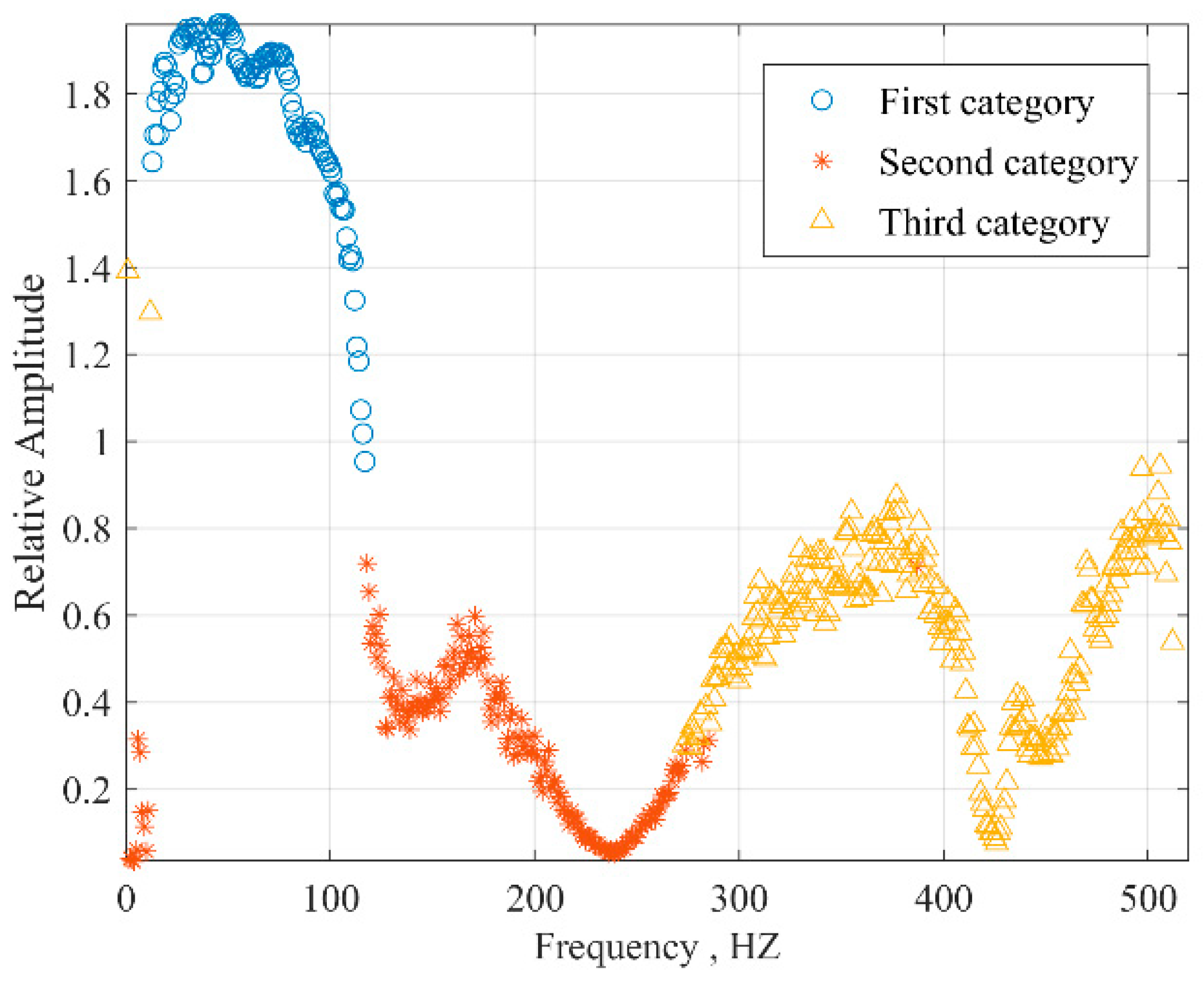
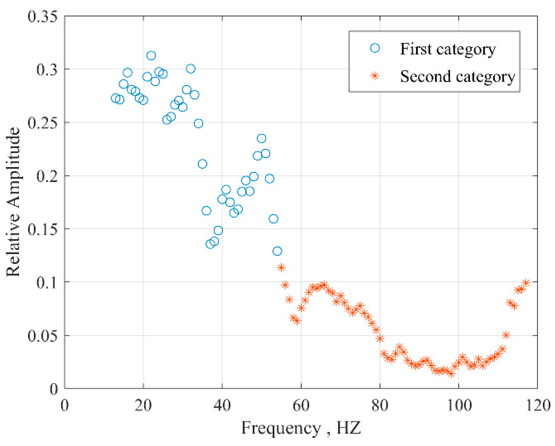
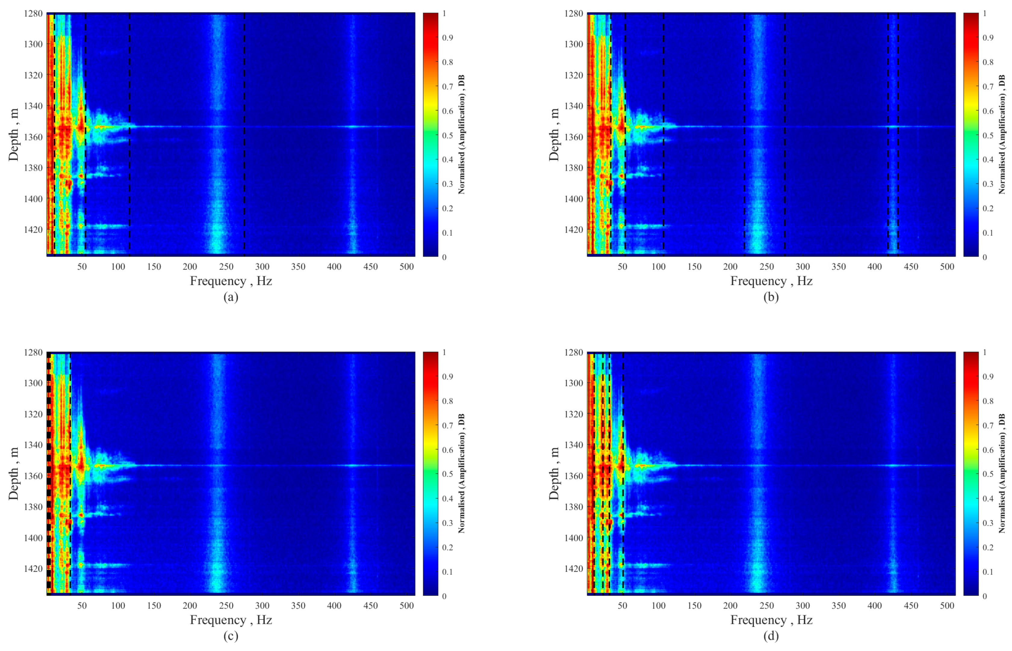
3.2. Vibration Signal Frequency Division Based on K-Means++ Algorithm

Fisher’s discriminant method is a linear discriminant method that can better distinguish individual totals based on the idea of analysis of variance and was proposed by Fisher in 1936. The discriminant method does not require any distribution of the totals. Fisher’s discriminant method is a projection method, which projects the points in the high-dimensional space to the low-dimensional space. It may be difficult to separate the samples in the original coordinate system, and the difference may be obvious after projection. Generally speaking, it is possible to project onto a one-dimensional space (a straight line) first, and if the result is not satisfactory, to project onto another straight line, thus constituting a two-dimensional space, and so on. A discriminant function can be established for each projection.
Fisher’s discriminant method was calculated for the distributed fiber optic vibration signal data from well A. The appropriate number of classifications was obtained as 3 classes. The vibration signal data [ X 1 , X 2 , , X m ] after data preprocessing were subjected to K-means++ clustering to obtain the effect graph shown in Figure 4.
From the clustering results of the distributed fiber optic vibration signals in Figure 4, it can be seen that the K-means++ algorithm roughly divides the frequency domain into 12–116 Hz, 116–275 Hz, and 275–512 Hz segments. The three types of clustered signals are well distinguished between the clusters, the average similarity within the clusters is high, and there are only a few discrete values in the very low frequency (0–12 Hz) signal interval. Therefore, in this paper, the distributed fiber optic vibration signal spectrum of well A is divided into three bands of 12–116 Hz, 116–275 Hz, and 275–512 Hz, which are named vibration signal bands I, II, and III, respectively.
The amplitude reflects the signal strength, and the average value of the amplitude of the vibration signals in the frequency bands I, II, and III was obtained to obtain the vibration signal curves of each of the three frequency bands of the distributed fiber optic vibration signals with the stratum, as shown in Figure 5 below:
As shown in Figure 5 above, the amplitude of the vibration signal in band I increases with depth. The amplitude of the vibration signal increases steeply at 1913 m until it reaches the peak at 1943 m, and then the amplitude decreases. The vibration signal of frequency band II is stronger at the surface. The amplitude increases steeply at 1933 m and then decreases to the normal gradient at 1953 m. The vibration signal of frequency band III is more gentle and is least affected by the depth of the stratum. The same amplitude peak exists in the depth section near 1943 m. Overall, the vibration signals of frequency bands I, II, and III all reach the highest amplitude value at a depth of 1943 m. The vibration signal of frequency band I has the strongest energy fluctuation, so it is presumed that the vibration signal of this band contains information on downhole fluid flow. The vibration signal of frequency band II has a higher amplitude than the vibration signal of frequency band I near the stratum, and the amplitude decreases gradually with an increase in depth and starts to be lower than the vibration signal of frequency band I at a depth of 1893 m, so it is presumed that the vibration signal of frequency band II represents the information of surface noise. The vibration signal of frequency band III is always low in amplitude compared with frequency bands I and II in the whole depth section, which is less influenced by the stratum and is consistent with the characteristics of the high-frequency band vibration signal, so it can be regarded as the base value of such a band vibration signal, i.e., background noise.
From the above data processing, it can only be inferred that the vibration signal of frequency band I contains the downhole fluid flow information, but it has not yet been determined which frequency band represents the downhole water absorption process and which frequency band can reflect the outside of the pipe trenching situation. Therefore, we needed to use the above-mentioned clustering method to perform secondary clustering of the vibration signal in frequency band I. The K-means++ clustering algorithm was set to 2. The clustering results of the two frequency bands of the distributed fiber optic vibration signal were obtained in the same way and named frequency bands 1 and 2, respectively, as shown in Figure 6.
From the above, Figure 6 can be obtained from the secondary clustering of the frequency band I vibration signal and divided into two intervals: 12–55 Hz and 55–116 Hz. The second clustering interval was named as one class of classification points and two classes of classification points, respectively. The vibration signal curves of one or two categories of classification points with the stratum were also obtained in the same way as the mean value of the amplitude, as shown in Figure 7.
In above Figure 7, the vibration curves of frequency bands 1 and 2 were obtained by secondary clustering. The vibration curve of No. 1 is the amplitude mean signal in the frequency band 12–55 Hz. The vibration curve of No. 2 is the amplitude rms signal in the frequency band of 55–116 Hz. It can be seen that the vibration curves of frequency bands 1 and 2 above 1913 m have similar vibration patterns, and the two curves almost overlap. At a depth of 1913 m, the amplitude of the vibration curve of the No. 2 band decreases to the local bottom, while the amplitude of the vibration curve of the No. 1 band starts to increase steeply, and the amplitude of the vibration curve of the No. 1 band is higher than that of the No. 2 band almost all the time after this depth. At a depth of 1943 m, the amplitude of the vibration curve of the No. 2 band reaches the peak and intersects with the vibration curve of the No. 1 band. At a depth of 1952 m and 1955 m, the amplitude of the No. 2 band vibration curve has been decreasing. At this time, the response signal of the vibration curve of the No. 1 band still exists, which is expressed in the form of two local peaks at depths of 1952 m and 1955 m, respectively. Accordingly, it is inferred that there is an extraneous flume in well A from 1913 m to 1955 m, and the vibration signal of the frequency band I contains the information of the downhole flume. The vibration curve of frequency band 2 indicates the reservoir flow signal, and the amplitude reaches the peak at 1943 m, where the main water absorption layer is.
In summary, the vibration signal data from well A are divided into frequency bands (see Table 1 for details), and the corresponding spectrograms can be obtained (see Figure 8). Among them, the ultra-low frequency signal (0–12 Hz) reflects the flow of fluid along the casing in the wellbore, while the low-frequency signal (12–55 Hz) reflects the flow through the injection section, the damaged area of the wellbore casing, and the aperture of the fracture in the cement ring. The medium-frequency signal (55–116 Hz) mainly reflects the flow of the reservoir, while the high-frequency signal (above 116 Hz) mainly represents the surface noise or background noise.
As shown in Figure 8 above, the A zone is in the 0–12 Hz band. The vibration signal in this zone is in the form of a longitudinal strip and is distributed throughout the well section, indicating the flow of fluid in the wellbore. The vibration signal in this zone is also in the longitudinal band and starts to fade to both sides from a depth of 1943 m. The strong vibration signal in this zone indicates the possible existence of cement ring trenching. The vibration signal in this zone has both transverse and longitudinal forms, the amplitude of the vibration signal is strongest at the surface in combination with the whole well, and the energy gradually decreases as the depth increases. In actual production, the well accurately determined the location of the leak point and the reservoir condition by combining the shut-in data and the open hole temperature, which was consistent with the above analysis results. This shows that the results of the K-means++ algorithm, by dividing the frequency bands to represent downhole events, have good correspondence with the actual production situation, and the method has good feasibility.

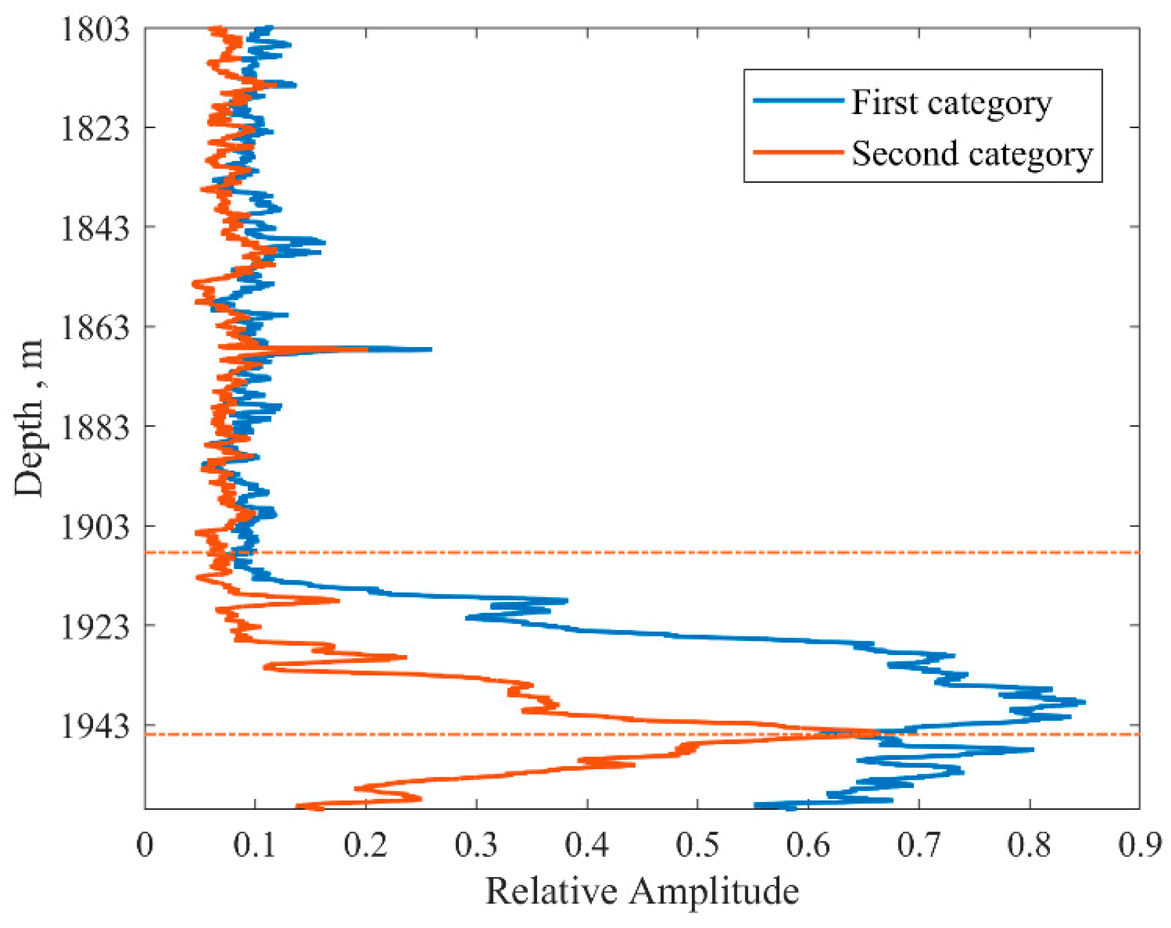
3.3. Production Estimation Analysis

The amplitude of the vibration signal is related to the flow rate, density, and viscosity of the fluid. Therefore, by analyzing the amplitude of the vibration signal, information about the downhole fluid motion can be obtained and, thus, the production of the well can be estimated [38,39].
Taking the actual production well B as an example, the completed drilling depth of well B is 1615 m, the inner diameter of the casing is 139.7 mm, the inner diameter of the tubing is 62 mm, the shot hole segments are all sandstone reservoirs, and the measured well section is 1282–1435 m. The measurement time is from 11:23:15 on 9 July 2022 to 10:51:36 on 10 July 2022, and the measured frequency domain is from 0 to 512 Hz. The distributed fiber vibration signal is converted into a spectrogram, and the vibration signal is divided into frequency bands using the K-means++ algorithm, as shown in Figure 9.
In Figure 9, the distribution of the vibration signals in zone A indicates the flow of fluids in the wellbore. Zone B shows longitudinal stripes at a depth of 1295–1430 m, and the intensity of the vibration signals in the upper part is greater than that in the lower part, which is judged as flow noise outside the tubing and may be a cement ring fugitive groove and mainly upward fugitive flow, with less fugitive flow in the lower part. Zone C shows horizontal stripes at 1354 m, 1381 m, and 1419 m. The vibration signal of the lateral stripes is judged to be the water absorption of the injection layer at 1354 m, the main water absorption at 1354 m, and less water absorption at 1381 m and 1419 m.
For well B, several other different clustering methods were compared. The specific frequency band range is shown in Table 2. Figure 10a demonstrates the K-means clustering used in this article, Figure 10b is K-medoids clustering, Figure 10c is hierarchical clustering, and Figure 10d is spectral clustering. In analyzing the clustering methods, K-means clustering is especially suitable for handling large datasets due to its efficiency and ease of implementation. Regarding the DAS clustering effects and comparing them with the production experience, Figure 10a shows that K-means clustering accurately categorizes the flow within the pipe. It is evident that at frequencies below 12 Hz, the distribution is consistently maintained from start to finish, while the classified leak frequency bands are only at mid-depth. Regarding the aspect of frequency division, Figure 10b’s K-medoids clustering combines the flow within the pipe and leaks; Figure 10c’s hierarchical clustering also only segments part of the flow within the pipe frequencies and combines some of the flow with some leaks; Figure 10d presents satisfactory results for the division of flow within the pipe and a more detailed classification of leaks. However, in actual production, such detailed distinctions of leaks are not created because the impact of different types of leaks at different frequency bands is the same. Notably, Figure 10b accurately classifies the surface noise, but since it is within an ineffective frequency band, these frequencies outside the reservoir fluids are not considered in actual production calculations. Upon comprehensive comparison, the advantages of K-means clustering become distinctly apparent.
It is known that the C-zone frequency band 55–116 Hz represents the reservoir fluid flow (Figure 9), and the corresponding vibration signal curve is obtained by averaging the amplitude for each depth point in this frequency band, as shown in Figure 11 below.
The envelope area of the main water absorption layer positions in the vibration signal curve was integrated and the water absorption was assigned according to the size of the envelope area of each layer, as shown in Table 3.
According to the well logging interpretation results of well B shown in Table 2, the fourth and fifth columns are borehole well interpretation data of porosity and permeability, respectively. By dividing the vibration signals in the frequency domain and calculating the envelope area of the vibration signals in each frequency band, the relative yield of the layer obtained was compared and analyzed with the relative water absorption data interpreted from the original production logging of the well. The results show that the interpreted results between the layers have good correspondence. Therefore, it can be concluded that the method of production interpretation by dividing the frequency bands of the distributed fiber optic vibration signals has high accuracy and can solve the problems in the actual production process. The method provides a quantitative basis for the interpretation of the production distribution among the layers.

4. Discussion

The practicality analysis shows that the method of observing the time–frequency diagram of a vibration signal has guiding significance for practical applications. And, there is a large blind spot in guiding practical applications based on the spectrum diagram alone. Therefore, in order to better guide the practical application, this paper proposes the idea of using the K-means++ algorithm to segment the vibration signals in frequency bands and extract the characteristics of vibration signals in different frequency bands to represent various event types in the well. It was found that the amplitude of the distributed fiber optic vibration signal is related to the flow rate size, while the frequency depends on the channel aperture. The fluid flow along the wellbore casing is represented in the spectrogram as ultra-low frequency (0–12 Hz) signals. Low-frequency (12–55 Hz) signals indicate the flow through the shot hole section, the damaged part of the wellbore casing, and the fracture aperture in the cement ring. Medium-frequency (55–116 Hz) signals contain the reservoir flow information, while high-frequency (above 116 Hz) signals correspond to the surface noise or background noise. A new vibration signal curve is constructed by calculating the average value of the amplitude of the frequency band that represents the fluid flow in the reservoir. Then, the curve is integrated to find the envelope area, and the relative yield of each layer can be obtained. The comparative analysis of experimental data and actual logging data proves that the method has good practicality and accuracy.
Distributed fiber optic vibration signal logging data processing and interpretation methods are based on the actual application environment; the disturbance signal is complex and diverse so only a small number of vibration signal types can be selected and have a characteristic degree of differentiation. In addition, distributed fiber optic vibration signal logging flow interpretation for multiphase fluids, especially oil, gas, and water, results in greater difficulties, so the interpretation method is mainly for single-phase fluids.

5. Conclusions

This paper introduces the basic principle and K-means++ algorithm of a distributed fiber optic vibration sensor. At the same time, to address the problem of blindness when the spectrum map guides the practical application, this paper proposes to segment the vibration signal frequency bands using the K-means++ algorithm and extract the vibration signal characteristics of different frequency bands to indicate various event types in the well. The relative production of each layer is indicated by finding the envelope area of the vibration signal curve indicating the frequency band of reservoir fluid flow, and the method has good practicality and accuracy in comparison with actual logging data.
Since the selected vibration signal types are fewer and have feature differentiation, a richer vibration dataset needs to be established to meet more complex and variable practical application scenarios in subsequent research. At the same time, the pattern recognition algorithm needs to be continuously optimized to improve the recognition accuracy and reliability of the algorithm.

Author Contributions

Y.G., W.Y. and X.D.: Conceptualization, Data curation, Methodology, Investigation, Validation, Writing—original draft. L.Z., Y.Z. and B.Y.: Supervision, Error analysis, Formal analysis, Resources, Writing—original draft and editing. Y.W. and R.D.: Supervision, Formal analysis, Funding acquisition, Resources, Writing—review and editing. All authors have read and agreed to the published version of the manuscript.

Funding

This research received no external funding.

Data Availability Statement

The data that support the findings of this study are available upon request from the corresponding author, R.D.

Conflicts of Interest

Yanan Guo and Xueqiang Dong were employed by the company PetroChina Qinghai Oilfield Company. Wenming Yang, Lei Zhang, Yue Zhang and Bo Yang were employed by the company PetroChina Tarim Oilfield Company. Author Yi Wang was employed by the company Sinopec Shengli Oilfield Company. The remaining authors declare that the research was conducted in the absence of any commercial or financial relationships that could be construed as a potential conflict of interest.

References

  1. Guo, H.-M.; Dai, J.-C.; Chen, K.-G. Principles of Production Logging and Data Interpretation; Petroleum Industry Press: Beijing, China, 2007; pp. 1–342. [Google Scholar]
  2. Soroush, M.; Mohammadtabar, M.; Roostaei, M.; Hosseini, S.A.; Fattahpour, V.; Mahmoudi, M.; Keough, D.; Tywoniuk, M.; Mosavat, N.; Cheng, L.; et al. Downhole Monitoring Using Distributed Acoustic Sensing: Fundamentals and Two Decades Deployment in Oil and Gas Industries. In Proceedings of the SPE Conference at Oman Petroleum & Energy Show, Muscat, Oman, 21–23 March 2022; OnePetro: Richardson, TX, USA, 2022. [Google Scholar]
  3. Horst, J.V.; Panhuis, P.I.; Al-Bulushi, N.; Deitrick, G.; Mustafina, D.; Hemink, G.; Groen, L.; Potters, H.; Mjeni, R.; Awan, K.; et al. Latest developments using fiber optic based well surveillance such as distributed acoustic sensing (DAS) for downhole production and injection profiling. In Proceedings of the SPE Kuwait Oil and Gas Show and Conference, Mishref, Kuwait, 12–15 October 2015; OnePetro: Richardson, TX, USA, 2015. [Google Scholar]
  4. Haavik, K.E. On the Use of Low-Frequency Distributed Acoustic Sensing Data for In-Well Monitoring and Well Integrity: Qualitative Interpretation. SPE J. 2022, 28, 1517–1532. [Google Scholar] [CrossRef]
  5. Parker, T.R.; Shatalin, S.V.; Farhadiroushan, M.; Miller, D. Distributed acoustic sensing: Recent field data and performance validation. In Second EAGE Workshop on Permanent Reservoir Monitoring 2013–Current and Future Trends; EAGE Publications BV: Utrecht, The Netherlands, 2013. [Google Scholar]
  6. Parker, T.; Shatalin, S.; Farhadiroushan, M. Distributed Acoustic Sensing–a new tool for seismic applications. First Break 2014, 32. [Google Scholar] [CrossRef]
  7. Ying, S.; Chang, W. Review of Distributed Optical Fiber Sensing Technology. J. Appl. Sci. 2021, 39, 843–857. [Google Scholar]
  8. Hayber, S.E.; Tabaru, T.E.; Keser, S.; Saracoglu, O.G. A Simple, High Sensitive Fiber Optic Microphone Based on Cellulose Triacetate Diaphragm. J. Light. Technol. 2018, 36, 5650–5655. [Google Scholar] [CrossRef]
  9. Keser, S.; Hayber, S.E. Fiber optic tactile sensor for surface roughness recognition by machine learning algorithms. Sens. Actuators A-Phys. 2021, 332, 113071. [Google Scholar] [CrossRef]
  10. Liu, J.; Lao, W.; Liang, W.; Liu, Q. A Wellbore Production Profile Monitoring Simulation Experiment Device Based on Distributed Fiber Optic Sound and Temperature Monitoring. CN201921116891.1, 16 July 2019. [Google Scholar]
  11. Leal-Junior, A.; Lopes, G.; Lazaro, R.; Duque, W.; Frizera, A.; Marques, C. SPR and FBG sensors system combination for salinity monitoring: A feasibility test. Opt. Fiber Technol. 2023, 78, 103305. [Google Scholar] [CrossRef]
  12. Beijing University. A Distributed Fiber Optic Acoustic Wave Sensing System and Its Sensing Method. CN201910748010.6, 14 August 2019.
  13. Madsen, K.N.; Thompson, M.; Parker, T.; Finfer, D. A VSP field trial using distributed acoustic sensing in a producing well in the North Sea. First Break. 2013, 31. [Google Scholar] [CrossRef]
  14. Barberan, C.; Allanic, C.; Avila, D.; Hy-Billiot, J.; Hartog, A.; Frignet, B.; Lees, G. Multi-Offset Seismic Acquisition Using Optical Fiber behind Tubing. In Proceedings of the 74th EAGE Conference and Exhibition incorporating EUROPEC 2012, Copenhagen, Denmark, 4–7 June 2012; EAGE Publications BV: Utrecht, The Netherlands, 2012. [Google Scholar]
  15. Tabatabaei, M.; Zhu, D. Fracture Stimulation Diagnostics in Horizontal Wells Using DTS. In Proceedings of the Canadian Unconventional Resources Conference, Calgary, Canada, 30 September–2 October 2014; OnePetro: Richardson, TX, USA, 2011. [Google Scholar]
  16. Kalia, N.; Gorgi, S.; Holley, E.; Cullick, A.S.; Jones, T. Wellbore Monitoring in Unconventional Reservoirs: Value of Accurate DTS Interpretation and Risks Involved. In Proceedings of the SPE Unconventional Resources Conference, The Woodlands, TX, USA, 1–3 April 2014; OnePetro: Richardson, TX, USA, 2014. [Google Scholar]
  17. Yu, G.; Sun, Q.; Ai, F.; Yan, Z.; Li, H.; Li, F. Micro-Structured Fiber Distributed Acoustic Sensing System for Borehole Seismic Survey. In Proceedings of the 2018 SEG International Exposition and Annual Meeting, Anaheim, CA, USA, 14–19 October 2018; OnePetro: Richardson, TX, USA, 2018. [Google Scholar]
  18. Wang, Y.; Li, M.; Li, X.; Wang, H.; Tian, L.; Deng, R. Identification and classification of water absorption profile of distributed optical fiber vibration signal based on XGBoost algorithm. SN Appl. Sci. 2022, 4, 289. [Google Scholar] [CrossRef]
  19. Liu, F.; Xie, S.; Gu, L.; He, X.; Yi, D.; Chen, Z.; Zhang, M.; Tao, Q. Common-mode noise suppression technique in interferometric fiber-optic sensors. J. Light. Technol. 2019, 37, 5619–5627. [Google Scholar] [CrossRef]
  20. Li, X.; Liu, X.; Zhang, Y.; Guo, F.; Wang, X.; Feng, Y. Application and progress of oil and gas well engineering monitoring technology based on distributed fiber optic acoustic sensing. Pet. Drill. Process 2022, 44, 309–320. [Google Scholar] [CrossRef]
  21. Anwar, I.; Carey, B.; Johnson, P.; Donahue, C. Detecting and Characterizing Fluid Leakage through Wellbore Flaws Using Fiber-Optic Distributed Acoustic Sensing. In Proceedings of the 56th US Rock Mechanics/Geomechanics Symposium, Santa Fe, NM, USA, 26–29 June 2022; OnePetro: Richardson, TX, USA, 2022. [Google Scholar]
  22. Bukhamsin, A.; Horne, R. Using Distributed Acoustic Sensors to Optimize Production in Intelligent Wells. In Proceedings of the SPE Annual Technical Conference and Exhibition, Amsterdam, The Netherlands, 27–29 October 2014; OnePetro: Richardson, TX, USA, 2014. [Google Scholar]
  23. Molenaar, M.M.; Hill, D.; Webster, P.; Fidan, E.; Birch, B. First downhole application of distributed acoustic sensing for hydraulic-fracturing monitoring and diagnostics. SPE Drill. Complet. 2012, 27, 32–38. [Google Scholar] [CrossRef]
  24. Thiruvenkatanathan, P.; Langnes, T.; Beaumont, P.; White, D.; Webster, M. Downhole Sand Ingress Detection Using Fibre-Optic Distributed Acoustic Sensors. In Proceedings of the Abu Dhabi International Petroleum Exhibition & Conference, Abu Dhabi, United Arab Emirates, 7–10 November 2016; OnePetro: Richardson, TX, USA, 2016. [Google Scholar]
  25. Boone, K.; Ridge, A.; Crickmore, R.; Onen, D. Detecting Leaks in Abandoned Gas Wells with Fibre-Optic Distributed Acoustic Sensing. In Proceedings of the IPTC 2014: International Petroleum Technology Conference, Doha, Qatar, 19–22 January 2014; EAGE Publications BV: Utrecht, The Netherlands, 2014. cp-395-00133. [Google Scholar]
  26. Wang, W. Design and Application of a Distributed Acoustic Sensing System for Logging. Master’s Thesis, University of Electronic Science and Technology, Chengdu, China, 2021. [Google Scholar] [CrossRef]
  27. Chen, T.; Guestrin, C. Xgboost: A Scalable Tree Boosting System; ACM: New York, NY, USA, 2016; pp. 785–794. [Google Scholar]
  28. McKinley, R.M.; Bower, F.M.; Rumble, R.C. The structure and interpretation of noise from flow behind cemented casing. J. Pet. Technol. 1973, 25, 329–338. [Google Scholar] [CrossRef]
  29. Xu, S. Noise logging. Logging Technol. 1980, 3, 18–28. [Google Scholar]
  30. Qiu, J.; Zhang, H.; Lei, G.; Wang, S.; Xie, F.; Gan, C. Application of noise spectrum logging in water injection wells. Logging Technol. 2017, 41, 601–605. [Google Scholar]
  31. Lin, Q.; Shen, K.; Jiang, Y.; Luo, Q.; Yao, J.; Tao, C. Application of continuous tubing distributed fiber optic logging technology in output profiles. Oil Gas Well Test. 2023, 32, 58–62. [Google Scholar]
  32. Cummins, H.Z.; Gammon, R.W. Rayleigh and Brillouin scattering in benzene: Depolarization factors. Appl. Phys. Lett. 1965, 6, 171–173. [Google Scholar] [CrossRef]
  33. Healey, P. Fading in heterodyne OTDR. Electron. Lett. 1984, 1, 30–32. [Google Scholar] [CrossRef]
  34. Koyamada, Y.; Imahama, M.; Kubota, K.; Hogari, K. Fiber-optic distributed strain and temperature sensing with very high measurand resolution over long range using coherent OTDR. J. Light. Technol. 2009, 27, 1142–1146. [Google Scholar] [CrossRef]
  35. Wang, Q.; Wang, C.; Feng, Z.; Ye, J. A review on the research of K-means clustering algorithm. Electron. Des. Eng. 2012, 20, 21–24. [Google Scholar]
  36. Wu, C.; Cheng, Y.; Zheng, Y.; Pan, Y. A review of K-means algorithm research. Mod. Libr. Inf. Technol. 2011, 5, 28–35. [Google Scholar]
  37. Wang, Y. Research on Distributed Fiber Optic Vibration Signal Logging Data Processing Method and Production Prediction. Master’s Thesis, Yangtze University, Jingzhou, China, 2023. [Google Scholar]
  38. Evans, R.P.; Blotter, J.D.; Stephens, A.G. Flow rate measurements using flow-induced pipe vibration. J. Fluids Eng. 2004, 126, 280–285. [Google Scholar] [CrossRef]
  39. Zhang, Y.K. Research on Fiber Optic Distributed Flow Monitoring Technology Based on backward Rayleigh Coherence. Master’s Thesis, Qilu University of Technology, Jinan, China, 2021. [Google Scholar]
Figure 1. Schematic diagram of distributed optical fiber vibration signal monitoring technology.
Processes 12 00721 g001
Figure 2. Well A distributed fiber optic vibration signal spectrogram.
Processes 12 00721 g002
Figure 3. Distributed fiber vibration signal spectrum diagram.
Processes 12 00721 g003
Figure 4. K-means++ algorithm was used to cluster distributed fiber vibration signal data.
Processes 12 00721 g004
Figure 5. Three frequency band vibration signal curves.
Processes 12 00721 g005
Figure 6. Secondary clustering partition.
Processes 12 00721 g006
Figure 7. Quadratic clustering vibration signal curve.
Processes 12 00721 g007
Figure 8. The spectrum diagram of well A divides frequency bands.
Processes 12 00721 g008
Figure 9. The spectrum diagram of well B divides frequency bands.
Processes 12 00721 g009
Figure 10. Comparison of practical application of clustering methods.
Processes 12 00721 g010
Figure 11. Vibration curve of reservoir fluid flow frequency band in well B.
Processes 12 00721 g011
Table 1. Comparison of filtering effects of different denoising algorithms.
NumberVibration SourceVibration Signal PatternFrequency RangeRemarks
1Flow in the tubeLongitudinal stripsLess than 12 HzFull well section distribution.
2Out-of-pipe run-off (cement run-off channel)Longitudinal strips12–55 HzExtends fading to both sides from the shot hole section and can be identified in combination with well temperature.
3Reservoir fluid flowHorizontal strips55–116 HzIt is related to the pore size, fracture angle, and openness and generally has a short extension, which may be divided into reservoir pore flow and reservoir fracture flow.
4Surface noiseNo fixed form116–275 HzThe amplitude is strongest at the surface and extends underground to fade away.
5Background noiseNo fixed formGreater than 275 HzHigh-frequency signals.
Table 2. Division results of different clustering methods.
NumberK-MeansK-MedoidsHierarchical ClusteringSpectral Clustering
1Less than 12 HzLess than 34 HzLess than 2 HzLess than 11 Hz
212–55 Hz34–54 Hz2–4 Hz11–23 Hz
355–116 Hz54–1074–6 Hz23–32 Hz
4116–275 Hz219–257 Hz, 418–432 Hz6–34 Hz32–51
5Greater than 275 Hz107–219 Hz, 257–418 Hz,
Greater than 432 Hz
Greater than 34 HzGreater than 51 Hz
Table 3. Shot hole data interpretation table.
NumberWell Section (m)Thickness (m)Porosity (%)Permeability (mD)Relative Water Absorption
(%)
Layer Relative Yield (%)
11345.6–1348.12.5221283.93.3
21351.7–1353.61.9211034.64.2
31355.4–1361.76.3221169.910.0
41363.4–1365.31.920872.32.2
51377.9–1385.07.121914.85.7
61387.4–1391.23.818452.32.3
71392.2–1394.11.9231590.50.9
81399.0–1404.85.818551.31.4
91415.3–1424.89.520758.98.3
Disclaimer/Publisher’s Note: The statements, opinions and data contained in all publications are solely those of the individual author(s) and contributor(s) and not of MDPI and/or the editor(s). MDPI and/or the editor(s) disclaim responsibility for any injury to people or property resulting from any ideas, methods, instructions or products referred to in the content.

