Fault Diagnosis of Wind Turbine Gearbox Using Vibration Scatter Plot and Visual Geometric Group Network

Abstract

This study aims to develop a fault detection system designed specifically for wind turbine gearboxes. It proposes a hybrid fault diagnosis algorithm that combines scatter plot analysis with the visual geometric group (VGG) technique to identify various fault types, including gear rust, chipping, wear, and aging. To capture vibration signals, a three-axis vibration sensor was integrated with a NI-9234 DAQ card. Digital signal processing techniques were employed to actively filter out noise from the captured signals. Gaussian white noise was incorporated into the training data to enhance the noise resistance of the network model, which was then utilized for scatter plot generation. The VGG technique was subsequently applied to identify faults. The testing data were collected at two different speeds, with 1500 samples taken at each speed, totaling 3000 samples. For both training and testing, 400 samples of each fault type were employed for training, while 200 samples were allocated for testing. The test results demonstrated an overall identification accuracy of 97.7% for both the no-fault gearbox and the four-fault states, underscoring the effectiveness of the proposed methodology.

1. Introduction

Reviewing research on fault detection in wind turbines, the primary components implicated in wind turbine faults encompass the blades [1], gearbox [2,3], bearings [4], and generator [5]. The gearbox, in particular, is a key component responsible for transmitting kinetic energy and increasing the speed of the blade rotor to match the generator’s operating speed. Dao et al. [6] reported that gearbox failures account for 7.5% of terrestrial wind turbine failures and 8.3% of offshore wind turbine failures. However, the downtime associated with gearbox failures constitutes 24.2% for terrestrial wind turbines and 33.3% for offshore wind turbines. Xiong et al. [7] observed that frequent occurrences of strong wind speeds severely impact gearboxes, complicating their dynamic response and leading to fatigue damage and bending fatigue failure. Bechhoefer et al. [8] discussed the measurement of vibration and rotational speed data from wind turbines and the development of an enhanced time synchronous average (TSA) to predict changes in the main rotor speed, thereby addressing issues such as icing or blade pitch errors. Qu et al. [9] compared the effectiveness of acoustic emission (AE) sensors and vibration sensors in diagnosing gear tooth cutting faults in gearboxes. Their findings suggest that AE performance is superior to, or at least equivalent to, vibration analysis. He et al. [10] utilized a large memory storage retrieval neural network (LAMSTAR) to diagnose bearing faults, including inner and outer races, rolling elements, and cage faults. The results indicated that LAMSTAR outperformed convolutional neural networks (CNN) in terms of fault recognition. Bechhoefer et al. [11] compared various condition indicators (CIs) for gear fault detection using a large dataset from three operational gearboxes and one faulty gearbox. The results demonstrated that selecting CIs with high statistical separability enhanced the sensitivity of the health indicator (HI). Peng et al. [12] introduced a health indicator, based on the noise-to-signal ratio (NSR) of current signals, to depict the gearbox’s health status. This method involved measuring the phase current of the generator linked to the gearbox and the root-mean-square value of vibration signals. A recurrent neural network (RNN) was trained using the real-time recurrent learning (RTRL) algorithm to forecast the health index. Subsequently, the predicted health index was compared with a predetermined threshold to assess the gearbox’s degradation. Huang et al. [13] employed three algorithms—support vector machine (SVM), particle swarm optimization (PSO), and decreasing step fruit fly optimization algorithm (DSFOA)—for diagnosing faults in wind turbine gearboxes. Initially, SVM was utilized to extract pivotal parameters from wind turbine fault vibration signals. Following this, DSFOA was employed to optimize SVM, and the combined approach was adopted for gearbox fault identification. The findings revealed that the accuracies of DSFOA-SVM and PSO-SVM were 93.33% and 90%, respectively. Liu et al. [14] introduced a sensitive component selection algorithm (SCSA), which integrates envelope spectral entropy and correlation coefficient to emphasize the fault characteristics of wind turbine gearboxes. Information entropy (IE) and dual-tree complex wavelet transform (DT-CWT) were employed to detect gearbox faults. The outcomes demonstrated the elimination of non-periodic components from signals at high frequencies and the extraction of sensitive components from early faults with subtle characteristics. Zhong et al. [15] proposed the pairwise-coupled sparse Bayesian extreme learning machine (PC-SBELM) for real-time fault diagnosis systems in wind turbine gearboxes. Fault features were derived using modified Hilbert–Huang transforms (HHT) and fed into the PC-SBELM for fault identification. Results illustrated an identification accuracy of 93.92%, with a processing time of 0.14 s. Among the deep learning methods, Amin et al. [16] proposed two approaches: cyclostationary-based CNN and kurtogram-based CNN. These methods proficiently detected low-speed shaft faults and assessed fault severity through simulation-based analyses, achieving 87% and 81.5% accuracy, respectively. Yu et al. [17] introduced the fast deep graph convolutional networks (FDGCNs) technique for adaptively learning fault features from initial graph inputs to diagnose vibration signal faults in wind turbine gearboxes, achieving a test accuracy of 93.09%. Pu et al. [18] proposed a deep enhanced fusion network (DEFN) utilizing vibration data from wind turbine gearboxes. Features were extracted using a sparse autoencoder (SAE) and enhanced via feature enhancement mapping (FEM). These features were then fused into the ensemble of shallow networks (ESN) for fault classification, with an identification accuracy of 79.05%. Qiu et al. [19] proposed a smart diagnosis method, based on deep convolutional neural networks (DCNNs), by conducting gearbox vibration experiments under various operating conditions and determining the gearbox vibration signal with optimal aging. Experimental results revealed an identification accuracy of 94.4% at a rotational speed of 1050 rpm.

VGG was selected for this study due to its capability to utilize smaller convolutional kernels to replace larger ones. This feature enables an increase in network depth and feature extraction capabilities. Additionally, it enhances the network’s nonlinear expression ability, without compromising the output results, even when maintaining the same number of parameters. This study measured vibration signals using an accelerometer to extract gearbox fault features. The proposed approach entails a hybrid algorithm combining a scatter plot and visual geometric group for identifying gearbox fault types, which included no-fault (Type A), rust (Type B), chipped (Type C), gearbox gear worn (Type D), and gearbox aged (Type E). Initially, the accelerometer was installed on the gearbox for signal capture, followed by signal processing to generate a scatter plot [20]. Subsequently, the scatter plot was utilized as a feature map input into VGG 19 for training and fault type identification [21].

2. Research System Architecture and Fault Design

This study focuses on detecting abnormal vibrations resulting from defects in wind turbine gearboxes. To achieve this, an experimental platform specifically for wind turbine gearbox testing was established. Figure 1 depicts the flow chart of the wind turbine gearbox testing experiment designed within this study. The wind turbine gearbox under examination was mounted on the experimental platform and operated at a constant speed. Vibration signals from the gearbox were captured using the KS943B.100 three-axis accelerometer, manufactured by Metra Mess- und Frequenztechnik (MMF) in Germany. Subsequently, a high-speed acquisition card captured the signals transmitted from the accelerometer. The unprocessed vibration signals underwent fast Fourier transform (FFT) and band-pass filtering. Following this, the two axes of the filtered three-axis vibration signals were transformed into the Cartesian coordinate system to generate a scatter plot. This scatter plot served as input for training the neural network. The trained model was then utilized to identify the type of fault present in the gearbox. Detailed specifications of the wind turbine measurement platform equipment are outlined in

Table 1. Wind turbine measurement platform equipment specifications.

Wind Turbine Measurement Platform Specifications
Induction motor	1.5 hp
Gearbox	1:12.25 gear ratio
Three-axis accelerometer (voltage sensitivity)	100 ± 5% (mV/g) sensitivity
NI-9234 DAQ (Manufactured by National Instruments in the U. S.)	51.2 kHz, 32-bit resolution, four synchronous channels

.

2.1. Fault Testing Platform and Gearbox Fault Design

This study developed a testing platform for gearbox faults, depicted in Figure 1. A single-phase motor propelled the platform, simulating the wind energy that propels wind turbine blades. The kinetic energy was then transmitted to the generator via the gearbox, resulting in the generation of electrical energy that is outputted from the generator to the load, facilitating effective energy utilization. A vibration sensor was mounted to the gearbox to capture real-time vibration signals, enabling analysis of the gearbox’s operational state and the detection of potential faults. As the single-phase motor propelled the gearbox to replicate wind energy, the vibration sensor continuously captured vibration signals, including the vibration features generated during gear operation, aiding the understanding of the gearbox’s operating condition. To facilitate precise fault diagnosis and condition monitoring, this study established five models: a no-fault gearbox (Type A) and four-faulty gearboxes (Types B to E), examining gearbox vibrations induced by faults. The specifications of the gearbox fault testing are outlined in

Table 2. Gearbox fault testing specifications.

Gearbox Fault Testing Specifications
Gearbox	Gear ratio 1:12.25
Gearbox fault types in wind turbines
Type A	No-fault
Type B	Rust
Type C	Chipped
Type D	Gear worn
Type E	Gear aged

.

2.1.1. No-Fault (Type A)

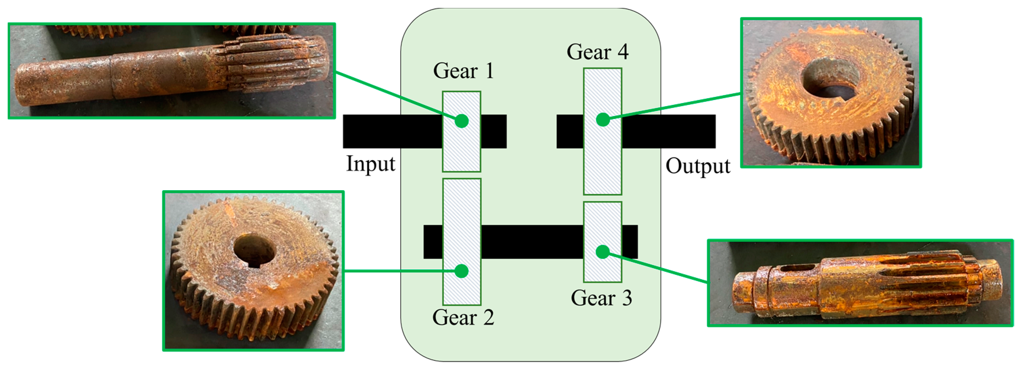
As the transmission equipment of the wind turbine, the gearbox plays a crucial role in power transmission. Wind energy is harnessed by the blades, causing them to rotate. However, wind-generated revolutions are insufficient for power generation. Hence, a gear speed increasing box is necessary to increase the speed until it reaches the rated speed of the generator. This study applied the proposed method to a scaled-down commercial gearbox, featuring a gear ratio of 12.25 and utilizing HD 220 lubricating oil, manufactured by Chinese Petroleum Corp. (CPC) in Taiwan. The physical entity and internal structure of the gearbox are illustrated in Figure 2.

In Figure 2a, $Z_1,Z_2,Z_3,Z_4$ represent the number of teeth of the four gears, while $f_A,f_B,f_C$ denote the rotation frequency. The relationship between rotation speeds of the input and output shaft is expressed as Equation (1).

$$f_A\frac{Z_1}{Z_2}\frac{Z_3}{Z_4}=\frac{Z_3}{Z_4}{f}_B=f_C$$

(1)

2.1.2. Rusty (Type B)

Lubricating oil is crucial in gearbox functionality, serving purposes such as lubrication, protection, cooling, and energy loss reduction. However, prolonged operation of wind turbines in harsh environments may lead to the infiltration of foreign substances like particles and water into the lubricating oil, causing deterioration and gear rusting [22]. Hence, this study developed a fault model specifically for gear rust to simulate the effects of water intrusion into the gearbox’s lubricating oil, as depicted in Figure 3.

2.1.3. Chipped (Type C)

Wind turbines are engineered to maximize efficiency and adeptly handle fluctuating wind directions. However, higher wind speeds can significantly impact the gearbox, especially with prolonged exposure to excessive and frequent wind speeds. Sudden extreme wind speeds can trigger complex dynamic responses within the wind turbine, subjecting the gearbox to considerable stress. The gear may chip or break when the forces exerted on the gear surpass the designed bearable load range. Additionally, prolonged usage or exposure to complex cyclic loads can lead to fatigue failure, resulting in gear chipping. Hence, Gear 1 and Gear 4 were intentionally damaged in this study to simulate gearbox chipping caused by extreme wind speeds, as shown in Figure 4.

2.1.4. Gear Worn (Type D)

When two gears mesh, the curved surfaces of their teeth contact each other and bear the load transmitted through the gear system. Excessive contact stress can result in local deformation and surface damage to the gear tooth surfaces. This manifests as contact spots characterized by high stress and pressure, leading to metal peeling, gear wear, and failure. Under heavy loads, the gears cannot mesh completely, causing the metal to peel off and resulting in gear wear. In this study, Gear 1, Gear 2, Gear 3, and Gear 4 were polished to replicate gear wear commonly observed within the gearbox, as depicted in Figure 5.

2.1.5. Gear Aged (Type E)

The performance and reliability of the gearbox degrades over time. Common damages include wear, material fatigue, and lubrication failure. Due to the challenges associated with repairing wind turbine gearboxes and the high maintenance costs involved, CNS 15176-1 specifies that the design life of a wind turbine gearbox should be a minimum of 20 years [23]. To simulate aging in this study, the gearbox model in Figure 2b was replaced by a gearbox that has been used for more than 20 years, provided by a company as an aging model, as shown in Figure 6.

3. Methodology

3.1. Signal Processing

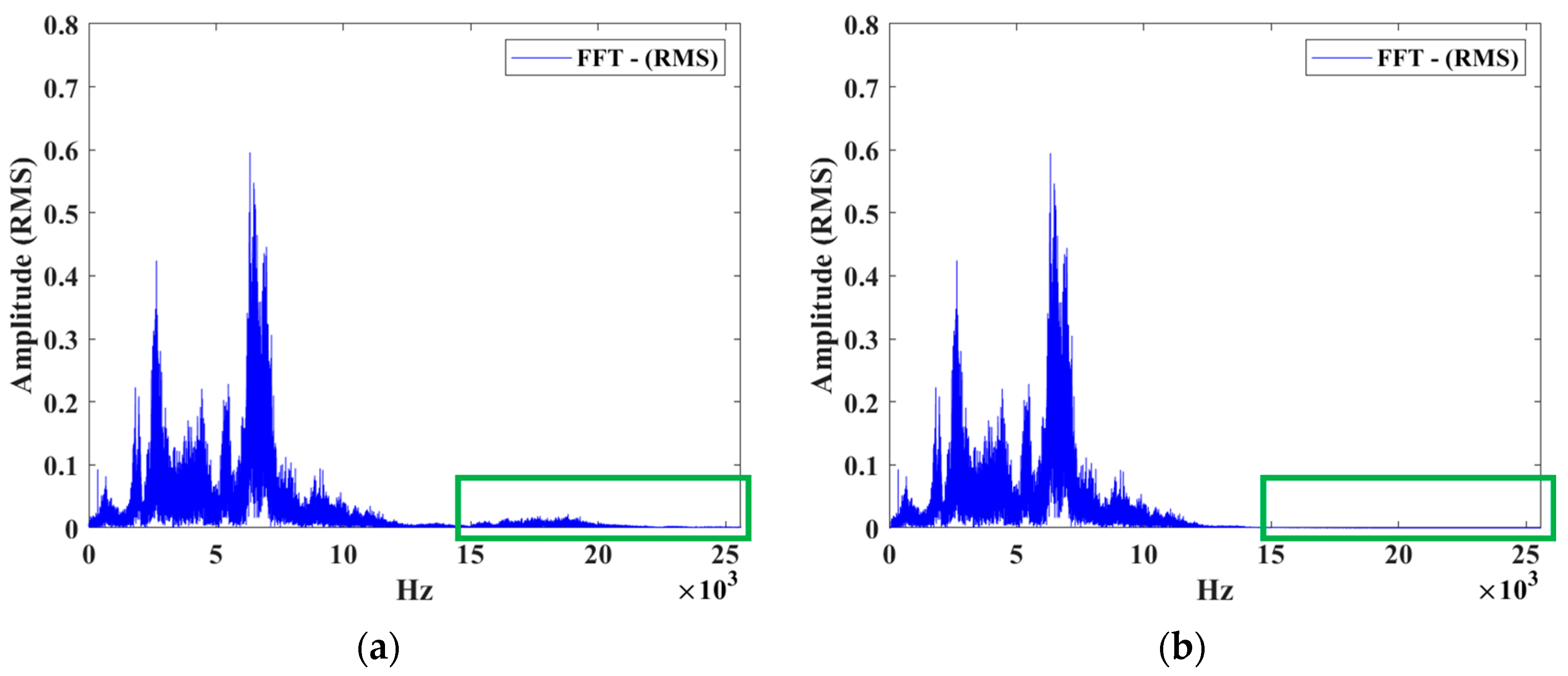
During vibration signal measurement, the ambient environment and electrical equipment introduce disturbances to the wind turbine. To enhance fault detection accuracy, the original signals underwent FFT in this study, converting the time domain signals into frequency domain signals. A band-pass filter was employed to filter the signals, effectively eliminating the power frequency interference below 60 Hz and the slight noise above 15 kHz, as shown in Figure 7. The green frame line in this figure denotes the removal of power-related interference and some unnecessary background noises, retaining only relatively obvious frequency signals between 60 Hz and 15 kHz.

3.2. Gaussian White Noise

Gaussian white noise is a common random signal, characterized by specific attributes in both the time and frequency domains and evenly distributed across the spectrum. Its generation follows the Gaussian distribution, resulting in values that exhibit randomness and continuity. Gaussian white noise maintains equal power density throughout the spectral range, showing no significant preference for specific frequencies. The noise intensity of Gaussian white noise is quantified by the signal-to-noise ratio (SNR), defined as the ratio of signal power to noise power, as expressed in Equation (2):

$$\mathrm{S}\mathrm{N}\mathrm{R}=\frac{{\mathrm{P}}_{\mathrm{s}\mathrm{i}\mathrm{g}\mathrm{n}\mathrm{a}\mathrm{l}}}{{\mathrm{P}}_{\mathrm{n}\mathrm{o}\mathrm{i}\mathrm{s}\mathrm{e}}}=\frac{{\mathrm{A}}_{\mathrm{s}\mathrm{i}\mathrm{g}\mathrm{n}\mathrm{a}\mathrm{l}}^2}{{\mathrm{A}}_{\mathrm{n}\mathrm{o}\mathrm{i}\mathrm{s}\mathrm{e}}^2}$$

(2)

The signal-to-noise ratio is represented by SNR, where ${\mathrm{P}}_{\mathrm{s}\mathrm{i}\mathrm{g}\mathrm{n}\mathrm{a}\mathrm{l}}$ represents the power of the signal, ${\mathrm{P}}_{\mathrm{n}\mathrm{o}\mathrm{i}\mathrm{s}\mathrm{e}}$ represents the power of the noise, ${\mathrm{A}}_{\mathrm{s}\mathrm{i}\mathrm{g}\mathrm{n}\mathrm{a}\mathrm{l}}$ represents the amplitude of the signal, and ${\mathrm{A}}_{\mathrm{n}\mathrm{o}\mathrm{i}\mathrm{s}\mathrm{e}}$ represents the amplitude of the noise. SNR is measured in decibels (dB), with the ratio of signal power to noise power represented by a tenfold logarithm, expressed as Equation (3):

$$\mathrm{S}\mathrm{N}\mathrm{R}\left(\mathrm{d}\mathrm{B}\right)=10{\log }_{10}(\frac{{\mathrm{P}}_{\mathrm{s}\mathrm{i}\mathrm{g}\mathrm{n}\mathrm{a}\mathrm{l}}}{{\mathrm{P}}_{\mathrm{n}\mathrm{o}\mathrm{i}\mathrm{s}\mathrm{e}}})=20{\log }_{10}(\frac{{\mathrm{A}}_{\mathrm{s}\mathrm{i}\mathrm{g}\mathrm{n}\mathrm{a}\mathrm{l}}}{{\mathrm{A}}_{\mathrm{n}\mathrm{o}\mathrm{i}\mathrm{s}\mathrm{e}}})$$

(3)

In this study, the training data were subjected to 5 dB noise, equivalent to approximately 30% of the SNR, while noise-free data were utilized for identification tests.

3.3. Scatter Plot

Scatter plots serve as visualizations of two-dimensional data distribution [24,25]. In a scatter plot, each data point corresponds to a set of observations of two variables, with one variable plotted on the horizontal axis and the other on the vertical axis. The relationship between variables is represented by their positions in a coordinate system. The scatter plot can present the distribution pattern, aggregation degree, and possible trends or correlations of data points. Figure 8 shows the scatter plot depicting the rusty state of the gearbox. This study incorporated this feature map into the convolutional neural network and VGG for training and type identification. Additionally, this study transformed the feature map into the snowflake diagram of the SDP proposed in [26] and imported it into the neural network for identification and comparison with the results of the scatter plot’s performance employed in this study.

3.4. Visual Geometric Group

VGG, a deep CNN architecture, treats image pixels as a group and employs the group theory transition matrix to describe geometric transformations. A transition matrix can be found for any geometric transformation, so that the transformed image is mapped onto the original group.

The VGG network architecture proposes the use of smaller 3 × 3 convolutional kernels to replace larger ones. This strategy can increase network depth and feature extraction capabilities, while enhancing the network’s nonlinear representation capacity under the same parameter count, thereby enhancing classification performance without affecting output results. Moreover, smaller convolutional kernels reduce the number of parameters in the network model, decreasing the computational load and accelerating the network training speed.

The VGG neural network introduces several convolutional layers, paired with a pooling layer in deep CNNs. This structure forms a convolution block that effectively extends the network’s depth and width, enhances the feature extraction capability, and improves the network’s classification performance. A VGG neural network’s convolution block typically contains 1–5 convolutional layers and one pooling layer, all using the same kernel size and stride to simplify the network model structure. The fully connected block usually comprises 1–3 fully connected layers, with the last layer being a softmax layer for classification.

3.4.1. VGG 19

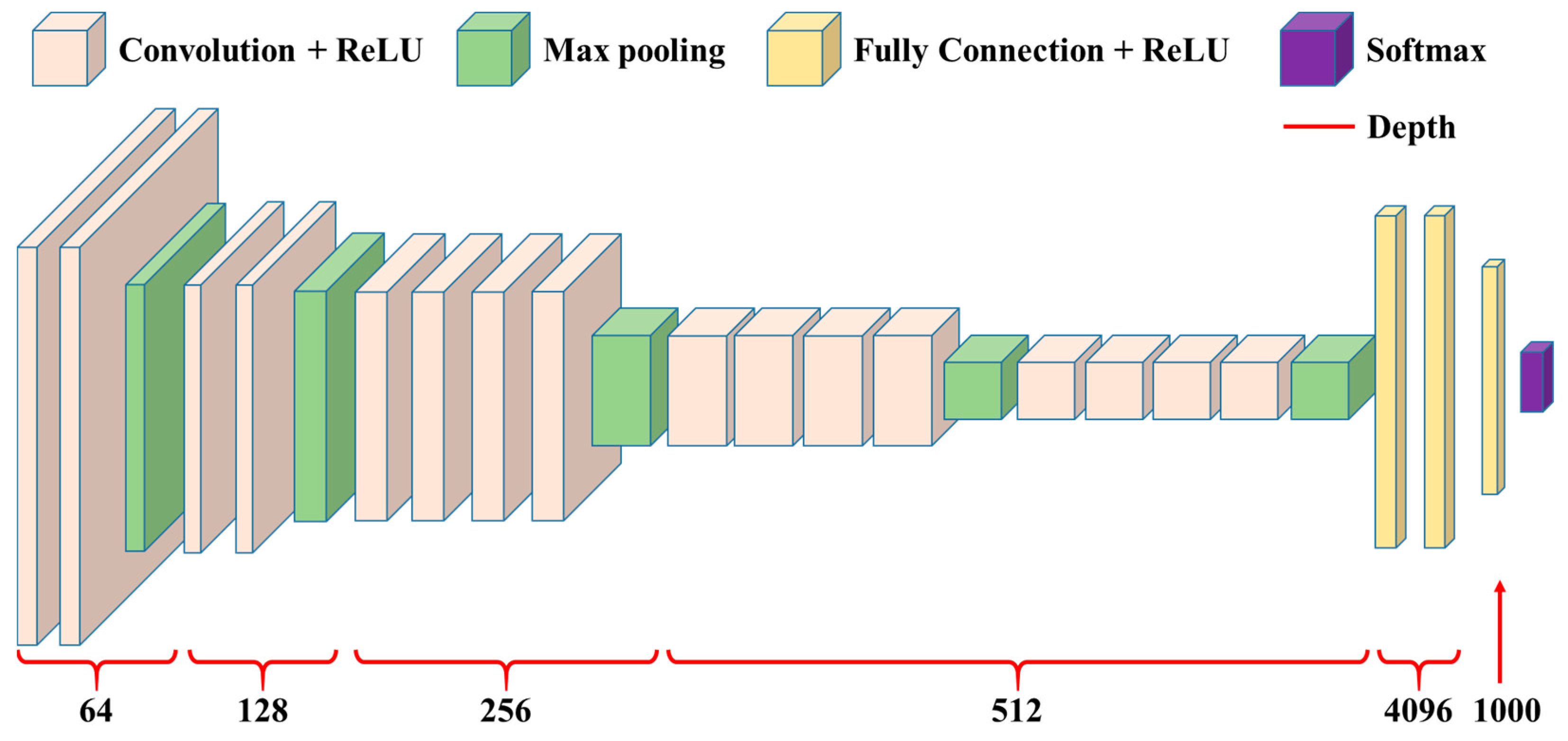
The network architecture of VGG 16 is relatively simple and intuitive, comprising 13 convolutional layers, three fully connected layers, and five max-pooling layers. The “16” signifies the combination of 13 convolutional layers and three fully connected layers. Similarly, VGG 19 consists of 16 convolutional layers, three fully connected layers, and five max-pooling layers. The network structure of VGG 19 is similar to that of VGG 16, comprising multiple convolutional and pooling layers stacked alternately. The image classification task is executed through several fully connected layers. Unlike VGG 16, VGG 19 comprises two sets of two convolutional layers and one max pooling layer, with three sets of four convolutional layers and one max pooling layer. The network depth of these convolution layers increases layer by layer. Small-sized convolutional kernels are used to enhance the nonlinear capability of the network model and increase its depth. Figure 9 illustrates the network architecture diagram of VGG 19. The network depth of the first and second convolutions is 64, while that of the third and fourth convolutions is 128. From the second to eighth convolutions, the network depth is 256, while that of the ninth to sixteenth convolutions is 256. Compared to VGG 16 (13 convolutional layers and three fully connected layers), VGG includes three more convolution layers, with a depth of 512, allowing for the extraction of numerous features from the input image.

3.4.2. Convolutional Kernel and Convolution Layer

In the VGG network model, the convolutional kernel is crucial to each convolution layer. The VGG network architecture comprises multiple convolution layers, with each employing a 3 × 3 convolutional kernel and utilizing the ReLU activation function, to enhance the network’s nonlinear properties. Increasing the network depth extracts more image features. The convolution layers in the VGG network model utilize the same padding convolution mode. This ensures that when the center of the convolutional kernel aligns with the corner of the input feature map, the convolution operation initiates, resulting in an output feature map size identical to the input feature map size. For instance, when conducting a convolution operation with a 3 × 3 kernel on a 4 × 4 image with a step size of 1, the depth corresponds to the network’s depth. The operation is then performed in groups, with corresponding grids multiplied in each operation. After scanning and calculating all target image pixels, the feature map is generated.

$${FM}_{out}=\frac{{FM}_{in}-f+2P}{Stride}+1$$

(4)

The calculation of the feature map size after the convolution operation is expressed as Equation (4), where ${FM}_{out}$ represents the output feature map size, ${FM}_{in}$ represents the input feature map size, $f$ represents the convolutional kernel size, $Stride$ represents the convolutional kernel movement step of each convolution, and $P$ represents the padding value of zero fill.

3.4.3. Pooling Layer

Pooling layers in the VGG network model reduce the size of the feature map, while retaining important feature information without changing the network depth. Max pooling is employed as the pooling method, effectively reducing the spatial size of the feature map while retaining significant feature information. By stacking convolution layers and pooling layers, the VGG network model extracts higher-level abstract feature representations, with convolution layers capturing local features and pooling layers reducing the size of the feature map, while retaining essential features.

3.4.4. Fully Connected Layer

The fully connected layer in the VGG network model architecture is located between the convolution block and the softmax function. It is responsible for the final classification or prediction of the features extracted from the convolution layer. VGG uses two fully connected layers, with 4096 neurons each, followed by one fully connected layer with 1000 neurons. The structure of the fully connected layer is shown in Figure 10. The softmax function calculates the probability distribution in the output layer.

Softmax is a mathematical function that can convert a K-dimensional vector into a K-dimensional probability distribution, ensuring each component falls between 0 and 1 and the sum equals 1. Commonly employed in multi-class classification problems, softmax converts the model’s output into a probability distribution. Its mathematical formula is presented in Equation (5), where $z$ denotes the vector,$z_i$ represents the $i$^th term of vector $z$, and $n$ denotes the number in the vector $z$. $Softmax\left(z_i\right)$ denotes the output probability distribution of the softmax function.

$$Softmax\left(z_i\right)=\frac{exp\left(z_i\right)}{{\sum }_{i=0}^{n}exp\left(z_i\right)}wherei=0,\dots ,n$$

(5)

4. Experimental Results

This study measured a one normal gearbox and four gearboxes with different faults. The gearbox operated at an input of 200 rpm, and vibration signals were captured along the X-axis and Y-axis, resulting in 300 vibration data points for each axis, totaling 600 vibration data points for both axes. With five gearbox types, a total of 3000 vibration signals were generated. Additionally, the gearbox operated at an input of 300 rpm, with the same data source as the 200-rpm condition. Therefore, in the mixed-speed gearbox, a total of 6000 vibration signals were generated. Subsequently, the two sets of vibration signals from the mixed-speed gearbox’s X-axis and Y-axis were used to create scatter plots, resulting in a total of 3000 scatter plots. Each gearbox type had 600 scatter plots. The total number of training samples was 400 scatter plots (200 for 200 rpm and 200 for 300 rpm), while the total number of testing samples was 200 scatter plots (100 for 200 rpm and 100 for 300 rpm).

4.1. Scatter Plot

This study captured time–domain vibration signals from five wind turbine gearbox models in operational states, using a high-speed data acquisition card. Subsequently, the noise was filtered out through back-end signal processing. The signal data from the X-axis and Y-axis were then mapped into a coordinate system, with the former serving as the independent and the latter as the dependent variables. These data were then used to create XY-axis scatter plots. Figure 11 illustrates the scatter plot of gearbox speeds at 200 rpm and 300 rpm. Notably, the scatter plot exhibits distinct changes when converting the signal from a rusty gearbox. Scatter plots depicting the no-fault gearbox and four types of faulty gearboxes offer ample visual differentiation for observing image disparities.

4.2. VGG 19

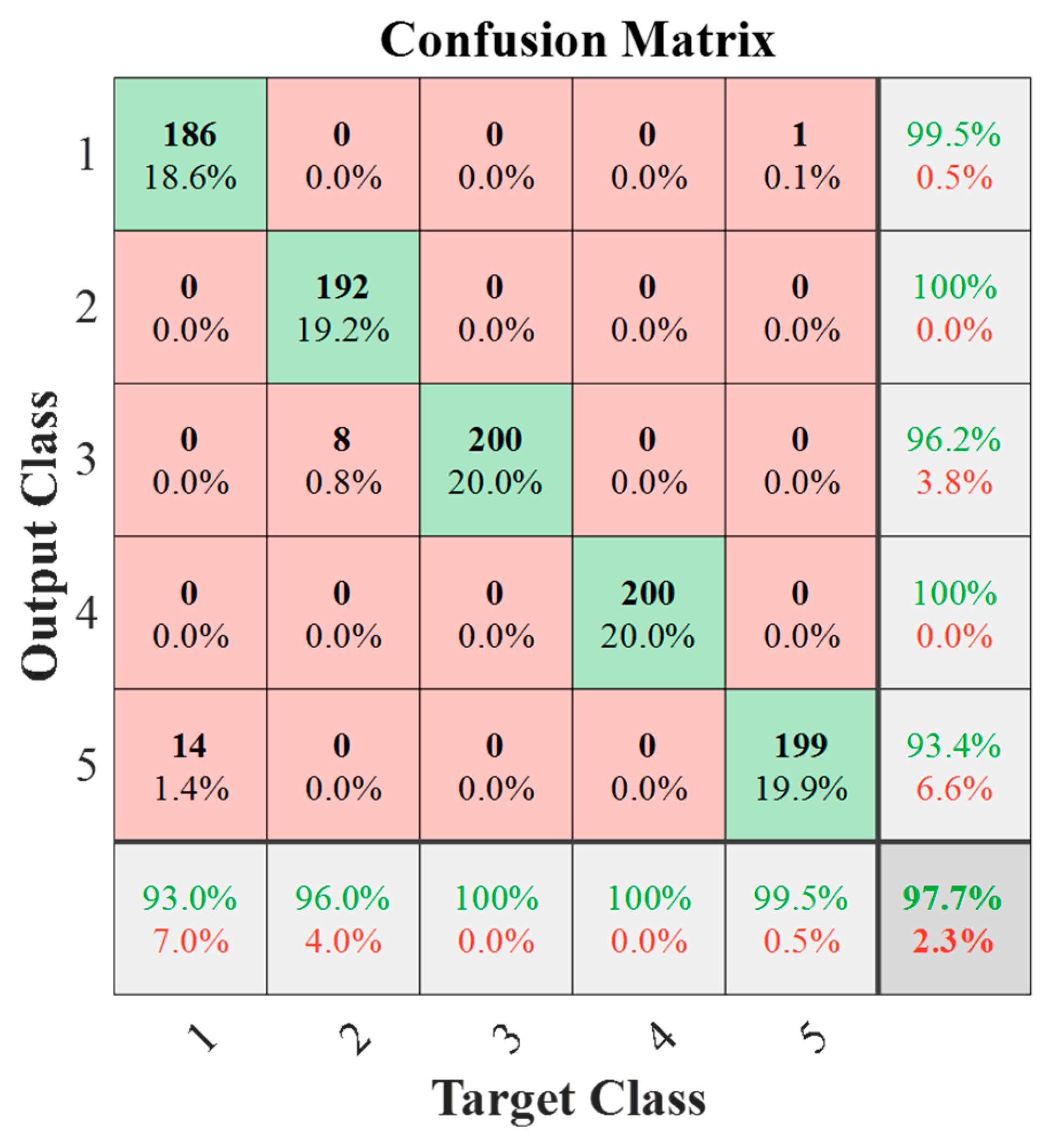
In this study, the vibration signals from the gearbox were converted into scatter plots to improve noise resistance in the trained neural network model. To simulate real-world conditions, 5 dB of noise was added to the training data, resulting in an SNR of approximately 30%. These noisy vibration signals were then converted into scatter plots and utilized as training samples for learning and training the VGG. On the other hand, the vibration signals without noise were also converted into scatter plots and fed into the trained VGG for identification purposes. Subsequently, the scatter plots were inputted into VGG 19 for learning and classification of the fault types. The identification results are summarized in a confusion matrix, as presented in

Table 3. Results of wind turbine gearbox fault identification based on VGG 19.

Fault Types	Training Pattern	Testing Pattern	Accuracy (%)
Type A	200	186	97.7
Type B	200	192
Type C	200	200
Type D	200	200
Type E	200	199

. Figure 12 displays the confusion matrix corresponding to the 5 dB noise level. For each fault type, the recognition rates were calculated based on the number of correctly identified samples out of the total test data samples. Specifically, Type A was correctly identified in 186 out of 200 test data samples, yielding a recognition rate of 93.0%. Similarly, the recognition accuracy rates for Type B, Type C, Type D, and Type E were 96.0%, 100%, 100%, and 99.5%, respectively. Ultimately, the total recognition accuracy of the system was determined to be 97.7%.

Table 4. Wind turbine gearbox fault identification performance comparison.

Algorithm	Training Time (s)	Testing Time (s)	Epoch	Accuracy (%)
				Non-Noise	5 dB
Scatter plot + VGG 19	95.2	0.0049	50	99.6	97.7
Scatter plot + VGG 19	228.4	0.0050	100	97.7	96.6
Scatter plot + VGG 19	344.0	0.0050	150	97.1	95.4
Scatter plot + VGG 16	93.2	0.0053	50	98.2	96.8
Scatter plot + VGG 16	156.5	0.0048	100	97.1	95.8
Scatter plot + VGG 16	223.5	0.0051	150	97.0	93.9
SDP + VGG 16	81.3	0.0049	50	92.1	85.5
SDP + VGG 19	100.1	0.0132	50	91.0	84.6
Scatter plot + CNN	85.1	0.0008	50	93.3	88.4
Scatter plot + HOG + SVM	4.2	0.19		87.3	79.2

presents the recognition results of the network model in this study. The epochs for the proposed method were set at 50, 100, and 150, to observe the experimental outcomes. At 100 epochs, the VGG 19 model achieved a recognition accuracy of 96.6% with 5 dB noise, requiring a training time of 228.4 s. Setting the epochs to 150 resulted in a recognition accuracy of 95.4% for VGG 19 with 5 dB noise, with a training duration of 344 s. In this case, setting the epochs to 50 yielded the best results, with a noise-free recognition accuracy of 99.6% and a recognition accuracy of 97.7% with 5 dB noise. Similarly, this study implemented scatter plots along with the VGG 16 recognition system, setting epochs at 50, 100, and 150, achieving recognition accuracies of 96.8%, 95.8%, and 93.9% with 5 dB noise, respectively.

The recognition accuracies with 5 dB noise for SDP, combined with VGG 16 and VGG 19, are 85.5% and 84.6%, respectively. These results indicate that the accuracy of scatter plots across different neural networks is consistently higher than that of SDP alone. Additionally, scatter plots were also inputted into a CNN for recognition, achieving a noise-free accuracy of 93.3% and a recognition accuracy of 88.4% with 5 dB noise. However, the highest recognition accuracy when using scatter plots combined with the traditional HOG + SVM was only 87.3%. From these results, it can be concluded that VGG 19 outperforms the others.

In terms of training time in deep learning methods, under the condition where epochs are set to 50, the SDP combined with the VGG 19 recognition system took about 100 s to complete training, making it the most time-consuming method among all recognition systems. Combining SDP with VGG 16 took 81.3 s, the shortest training time among all systems. Finally, the recognition time spent by all systems was less than one second, demonstrating that using different feature maps and neural networks for recognition does not significantly impact the testing time.

To evaluate the performance of different algorithms’ models, various indicators were used to calculate the model’s evaluation scores [27]. Four classification indicators can be obtained from the confusion matrix: true positives (TPs), false positives (FPs), false negatives (FNs), and true negatives (TNs). TPs represent cases where the actual samples are positive and predicted as positive. FPs denote cases where the actual samples are negative but misjudged as positive. FNs refer to cases where the actual samples are positive but misjudged as negative. TNs indicate cases where the actual samples are negative and predicted as negative. Calculating these four classification indicators yields evaluation metrics such as precision, recall, F1-score, and kappa, as shown in Equations (6)–(9).

Precision represents the proportion of correctly predicted positive samples among all those predicted as positive. Recall indicates the proportion of actual positives that were correctly predicted. The F1-score represents the harmonic mean of precision and recall, serving as a standard measure of test accuracy. Meanwhile, kappa is a statistical measurement used to determine the consistency between model predictions and actual classification outcomes. In Equation (9), ${\mathrm{p}}_{\mathrm{o}}$ represents the overall accuracy of the model while ${\mathrm{p}}_{\mathrm{e}}$ represents the level of consistency between the model’s predictions and actual class values, calculated as the sum of the product of the actual counts of each class and their predicted counts, divided by the square of the total number of all classes.

In this study, the accuracy with 5 dB noise was used to calculate the model evaluation metrics for different algorithms, and the results are summarized in

Table 5. Model evaluation metrics for different algorithms.

Algorithm	Accuracy (%)	Precision	Recall	F1-Score	Kappa
Scatter plot + VGG 19	97.7	0.9947	0.930	0.9612	0.971
Scatter plot + VGG 19	96.6	0.9946	0.920	0.9558	0.958
Scatter plot + VGG 19	95.4	0.9891	0.910	0.9479	0.943
Scatter plot + VGG 16	96.8	0.9946	0.915	0.9531	0.960
Scatter plot + VGG 16	95.8	0.9943	0.870	0.9280	0.948
Scatter plot + VGG 16	93.9	0.9836	0.900	0.9399	0.924
SDP + VGG 16	85.5	0.8458	0.850	0.8479	0.819
SDP + VGG 19	84.6	0.8458	0.850	0.8479	0.808
Scatter plot + CNN	88.4	0.6491	0.925	0.7629	0.855
Scatter plot + HOG + SVM	79.2	0.5217	0.900	0.6606	0.740

. Taking Figure 12 as an example, the problem focuses on the presence or absence of faults, constituting a binary classification. In the no-fault category, TP, FP, FN, and TN values are 186, 1, 14, and 799, respectively. Therefore, the precision is 0.9947, recall is 0.93, F1-score is 0.9612, and kappa is calculated as 0.971, where ${\mathrm{p}}_{\mathrm{o}}$ is 0.977 and ${\mathrm{p}}_{\mathrm{e}}$ is 0.2.

$$\mathrm{P}\mathrm{r}\mathrm{e}\mathrm{c}\mathrm{i}\mathrm{s}\mathrm{i}\mathrm{o}\mathrm{n}=\frac{\mathrm{T}\mathrm{P}}{\mathrm{T}\mathrm{P}+\mathrm{F}\mathrm{P}}$$

(6)

$$\mathrm{R}\mathrm{e}\mathrm{c}\mathrm{a}\mathrm{l}\mathrm{l}=\frac{\mathrm{T}\mathrm{P}}{\mathrm{T}\mathrm{P}+\mathrm{F}\mathrm{N}}$$

(7)

$$\mathrm{F}1-\mathrm{s}\mathrm{c}\mathrm{o}\mathrm{r}\mathrm{e}=2\times \frac{\mathrm{P}\mathrm{r}\mathrm{e}\mathrm{c}\mathrm{i}\mathrm{s}\mathrm{i}\mathrm{o}\mathrm{n}\times \mathrm{R}\mathrm{e}\mathrm{c}\mathrm{a}\mathrm{l}\mathrm{l}}{\mathrm{P}\mathrm{r}\mathrm{e}\mathrm{c}\mathrm{i}\mathrm{s}\mathrm{i}\mathrm{o}\mathrm{n}+\mathrm{R}\mathrm{e}\mathrm{c}\mathrm{a}\mathrm{l}\mathrm{l}}$$

(8)

$$\mathrm{K}\mathrm{a}\mathrm{p}\mathrm{p}\mathrm{a}=\frac{{\mathrm{p}}_{\mathrm{o}}-{\mathrm{p}}_{\mathrm{e}}}{1-{\mathrm{p}}_{\mathrm{e}}}$$

(9)

5. Conclusions

This study proposes a fault diagnosis method for wind turbine gearboxes by integrating scatter plots and VGG 19. The system diagnoses gearbox faults by extracting fault features from vibration signals. Five gearbox fault states were considered: no-fault, rust, chipping, wear, and aging. Gaussian white noise was added to the training data to enhance the network’s noise resistance. Fault identification was conducted using VGG 19, with test results showing an accuracy of 97.7% in identifying the no-fault and four fault states of the gearbox, confirming the method’s effectiveness. The study also examined model performance under different epoch settings, revealing optimal results with 50 epochs. Additionally, comparison with VGG 16 demonstrated the superior performance of VGG 19, effectively extracting gearbox fault features and improving diagnostic accuracy. This technology holds potential for application in fault diagnostics of other components in the future.

References

1. Liu, Z.; Wang, X.; Zhang, L. Fault Diagnosis of Industrial Wind Turbine Blade Bearing Using Acoustic Emission Analysis. IEEE Trans. Instrum. Meas. 2020, 69, 6630–6639. [Google Scholar] [CrossRef]
2. He, Q.; Zhao, J.; Jiang, G.; Xie, P. An Unsupervised Multiview Sparse Filtering Approach for Current-Based Wind Turbine Gearbox Fault Diagnosis. IEEE Trans. Instrum. Meas. 2020, 69, 5569–5578. [Google Scholar] [CrossRef]
3. Assoumane, A.; Ravier, P.; Capdessus, C.; Sekko, E. H∞ estimator for gearbox diagnosis in variable speed conditions. In Proceedings of the 2017 25th European Signal Processing Conference (EUSIPCO), Kos, Greece, 28 August–2 September 2017. [Google Scholar]
4. Huang, N.; Chen, Q.; Cai, G.; Xu, D.; Zhang, L.; Zhao, W. Fault Diagnosis of Bearing in Wind Turbine Gearbox Under Actual Operating Conditions Driven by Limited Data with Noise Labels. IEEE Trans. Instrum. Meas. 2021, 70, 3502510. [Google Scholar] [CrossRef]
5. Artigao, E.; Honrubia-Escribano, A.; Gómez-Lázaro, E. In-Service Wind Turbine DFIG Diagnosis Using Current Signature Analysis. IEEE Trans. Ind. Electron. 2020, 67, 2262–2271. [Google Scholar] [CrossRef]
6. Dao, C.; Kazemtabrizi, B.; Crabtree, C. Wind turbine reliability data review and impacts on levelised cost of energy. Wind Energy 2019, 22, 1848–1871. [Google Scholar] [CrossRef]
7. Xiong, Z.; Qiu, Y.; Feng, Y.; Chen, L. Fatigue Damage of Wind Turbine Gearbox Under Extreme Wind Conditions. In Proceedings of the 2018 Prognostics and System Health Management Conference (PHM-Chongqing), Chongqing, China, 26–28 October 2018. [Google Scholar]
8. Bechhoefer, E.; Wadham-Gagnon, M.; Boucher, B. Initial Condition Monitoring Experience on a Wind Turbine. Annu. Conf. PHM Soc. 2012, 4, 63–70. [Google Scholar] [CrossRef]
9. Qu, Y.; He, D.; Yoon, J.; Van Hecke, B.; Bechhoefer, E.; Zhu, J. Gearbox Tooth Cut Fault Diagnostics Using Acoustic Emission and Vibration Sensors—A Comparative Study. Sensors 2014, 14, 1372–1393. [Google Scholar] [CrossRef]
10. He, M.; He, D.; Bechhoefer, E. Using Deep Learning Based Approaches for Bearing Fault Diagnosis with AE Sensors. Annu. Conf. PHM Soc. 2016, 8, 282–291. [Google Scholar] [CrossRef]
11. Bechhoefer, E.; Butterworth, B. A Comprehensive Analysis of the Performance of Gear Fault Detection Algorithms. Annu. Conf. PHM Soc. 2019, 11, 1–11. [Google Scholar] [CrossRef]
12. Peng, Y.; Cheng, F.; Qiao, W.; Qu, L. Fault prognosis of drivetrain gearbox based on a recurrent neural network. In Proceedings of the 2017 IEEE International Conference on Electro Information Technology (EIT), Lincoln, NE, USA, 14–17 May 2017. [Google Scholar]
13. Huang, C.; Li, Y.; Zhang, T.; Hou, G.; Zhang, J. Fault diagnosis of wind turbine gearbox by diminishing step fruit fly algorithm optimized SVM. In Proceedings of the 2017 Chinese Automation Congress (CAC), Jinan, China, 20–22 October 2017. [Google Scholar]
14. Liu, Q.; Yang, J. Fault Diagnosis of Wind Turbine Gearbox Based on Dual-tree Complex Wavelet and Information Entropy. In Proceedings of the 2018 Prognostics and System Health Management Conference (PHM-Chongqing), Chongqing, China, 26–28 October 2018. [Google Scholar]
15. Zhong, J.H.; Zhang, J.; Liang, J.; Wang, H. Multi-Fault Rapid Diagnosis for Wind Turbine Gearbox Using Sparse Bayesian Extreme Learning Machine. IEEE Access 2019, 7, 773–781. [Google Scholar] [CrossRef]
16. Amin, A.; Bibo, A.; Panyam, M.; Tallapragada, P. Vibration-based Condition Monitoring in Wind Turbine Gearbox Using Convolutional Neural Network. In Proceedings of the 2022 American Control Conference (ACC), Atlanta, GA, USA, 8–10 June 2022. [Google Scholar]
17. Yu, X.; Tang, B.; Zhang, K. Fault Diagnosis of Wind Turbine Gearbox Using a Novel Method of Fast Deep Graph Convolutional Networks. IEEE Trans. Instrum. Meas. 2021, 70, 6502714. [Google Scholar] [CrossRef]
18. Pu, Z.; Li, C.; Zhang, S.; Bai, Y. Fault Diagnosis for Wind Turbine Gearboxes by Using Deep Enhanced Fusion Network. IEEE Trans. Instrum. Meas. 2021, 70, 2501811. [Google Scholar] [CrossRef]
19. Qiu, G.; Gu, Y.; Cai, Q. A deep convolutional neural networks model for intelligent fault diagnosis of a gearbox under different operational conditions. Measurement 2019, 145, 94–107. [Google Scholar] [CrossRef]
20. Rapp, T.; Peters, C.; Dachsbacher, C. Visual Analysis of Large Multivariate Scattered Data using Clustering and Probabilistic Summaries. IEEE Trans. Visual Comput. Graphics. 2021, 27, 1580–1590. [Google Scholar] [CrossRef] [PubMed]
21. Pangilinan, J.R.; Legaspi, J.; Linsangan, N. InceptionV3, ResNet50, and VGG19 Performance Comparison on Tomato Ripeness Classification. In Proceedings of the 2022 5th International Seminar on Research of Information Technology and Intelligent Systems (ISRITI), Yogyakarta, Indonesia, 8–9 December 2022. [Google Scholar]
22. Singh, D.K.; Kurien, J.; Villayamore, A. Study and analysis of wind turbine gearbox lubrication failure and its mitigation process. Mater. Proc. 2021, 44, 3976–3983. [Google Scholar] [CrossRef]
23. CNS15176-1: Wind Turbines—Part 1: Design Requirements. Available online: https://www.cnsonline.com.tw/?node=detail&generalno=15176-1&locale=en_US (accessed on 11 May 2024).
24. Wang, X.; Yang, C.; Zhang, Z.; Du, Y. DCT-Based Deep Learning of Polarimetric Scattering from a Dielectric Cylinder. IEEE Geosci. Remote Sens. Lett. 2022, 19, 4021905. [Google Scholar] [CrossRef]
25. Pang, X.Y.; Tong, Y.; Zhang, B.W.; Wei, J.G. NSP-CNN Rolling Bearing Fault Diagnosis Method. In Proceedings of the 2021 Global Reliability and Prognostics and Health Management (PHM-Nanjing), Nanjing, China, 15–17 October 2021. [Google Scholar]
26. Zhu, X.; Zhao, J.; Hou, D.; Han, Z. An SDP characteristic information fusion-based CNN vibration fault diagnosis method. Shock Vib. 2019, 2019, 3926963. [Google Scholar] [CrossRef]
27. Ahmad, S.; Choudhury, P.K. On the Performance of Deep Transfer Learning Networks for Brain Tumor Detection Using MR Images. IEEE Access 2022, 10, 59099–59114. [Google Scholar] [CrossRef]
Figure 1. Gearbox testing platform and experiment flow chart.
Processes 12 00985 g001
Figure 2. No-fault gearbox model: (a) schematic diagram of the gearbox; (b) stereogram of the gearbox.
Processes 12 00985 g002
Figure 3. Schematic diagram of the rusty gear model.
Processes 12 00985 g003
Figure 4. Schematic diagram of the chipped gear model.
Processes 12 00985 g004
Figure 5. Schematic diagram of gear worn model.
Processes 12 00985 g005
Figure 6. Aged gearbox model.
Processes 12 00985 g006
Figure 7. Analysis of the spectrum of 300 rpm vibration signals from a gearbox experiencing rust. (a) Unfiltered spectrum; (b) filtered spectrum.
Processes 12 00985 g007
Figure 8. Scatter plot of the rusty state of the wind turbine gearbox.
Processes 12 00985 g008
Figure 9. VGG 19 architecture.
Processes 12 00985 g009
Figure 10. The architecture of the VGG fully connected layer.
Processes 12 00985 g010
Figure 11. Scatter plot of the gearbox fault model. (a) Scatter plot of the no-fault gearbox at 200 rpm; (b) scatter plot of the rusty gearbox at 200 rpm; (c) scatter plot of the chipped gearbox at 200 rpm; (d) scatter plot of the gear worn gearbox at 200 rpm; (e) scatter plot of the gear aged gearbox at 200 rpm; (f) scatter plot of the no-fault gearbox at 300 rpm; (g) scatter plot of the rusty gearbox at 300 rpm; (h) scatter plot of the chipped gearbox at 300 rpm; (i) scatter plot of the gear worn gearbox at 300 rpm; (j) scatter plot of the gear aged gearbox at 300 rpm.
Processes 12 00985 g011aProcesses 12 00985 g011b
Figure 12. The confusion matrix with 5 dB noise.
Processes 12 00985 g012