Static Characteristics and Energy Consumption of the Pressure-Compensated Pump

Abstract

The motivation of this research was to assess the possibility of speed control for the selected pressure-compensated pump. Measured static characteristics of an axial piston pump with pressure compensation are presented in the paper. Based on these characteristics, the pump efficiencies are determined. The characteristics and efficiencies are determined for the different pump outlet pressures, pump speeds, relative displacements and for the different pressures set at the pressure compensator. In addition, the different methods of pump control were compared. These are displacement control, speed control and both controls. The efficiency of each control method was compared based on the determined mechanical input power at the pump drive shaft. By comparing these control methods, it was found that the combination of both control methods can achieve up to 93% savings of mechanical power in the controlled state (stand-by state). Also, the adverse effects resulting from each control method that reduces pump efficiency were defined.

1. Introduction

Axial piston pressure-compensated pumps are used in hydraulic systems with higher powers. Their design allows to change the displacement. When there is no demand for fluid flow (stand-by state), a decrease in displacement leads to a decrease in flow at constant pump speed and constant pressure. This achieves a reduction in pump power loss. Pump speed control is another way to decrease the flow rate. Decreasing the pump speed will decrease the flow rate at constant displacement and constant pressure. For this control method, an electric motor controlled by a frequency converter, a pressure sensor at the pump outlet and an electronic controller are required. In the case of displacement control, the control is provided by a hydraulic–mechanical pressure compensator.

During the control process, the pump parameters change, whether it is the pump displacement or the pump speed. These changes affect the pump efficiency, which varies depending on the current boundary conditions [1,2,3]. In order to compare the different types of control, it is necessary to determine the pump characteristics and efficiencies for the different operating conditions that may occur during and after pump control [4].

The authors of the article [1] discuss the possibility of speed control and displacement control. In their results, it is summarized that after the displacement control from the maximum value to the minimum value and the subsequent speed control from 1800 min⁻¹ to 300 min⁻¹, it is possible to save 83% of the original input power. Displacement control and speed control are also addressed in the study in [2]. Their results show that by reducing the speed from 1500 min⁻¹ to 300 min⁻¹, they saved 3 kW of input power in their case. The authors of the study [3] are focused on speed control (VSPM), displacement control (VDPM) and combination of both controls (VSDPM). From their results, it can be seen that in the VDPM stand-by state, the system power is 1.493 kW and in the VSDPM stand-by state, the system power is 0.046 kW. It is also described that VSPDM achieves better efficiency for lower speeds and low loads than VPDM. The authors of the paper [4] show in their study that the power consumption when the pump does not supply flow is a system power of 2.67 kW when only displacement control is implemented. When both controls are implemented, the system power reaches 0.62 kW.

Furthermore, the results of the study in [5] show that the mechanical pressure efficiency increases with increasing pump outlet pressure and that the mechanical pressure efficiency decreases with increasing pump speed. In contrast, the flow efficiency decreases with increasing pressure and increases with increasing speed. These facts are also the conclusion of the studies in articles [6,7,8,9,10]. Similar conclusions for other pump designs were reached by the authors in articles [11,12,13,14,15,16]. The volumetric efficiency depends on the leakage flow, i.e., the flow rate losses. The leakage of axial piston pumps is mentioned by the authors in the article [17]. They conclude that up to 94% of all leakage is produced between the slipper and swash plate or between the barrel and port plate. The volumetric efficiency was also investigated by the authors in the paper [18] and from their results, it can be seen that the volumetric efficiency increases with increasing pump speed. Volumetric efficiency also depends on the contamination of the fluid [19].

An important part of a pressure-compensated pump is the pressure compensator and therefore a few studies dealing with pressure compensators are presented in this paper. Characteristics of the pressure compensator are investigated by the authors in the paper [20], and from the results, it can be seen that the pressure increase can take values of p_i = 5 bar. In the paper [21], the characteristics and optimization of the power control valve are investigated. It is concluded that the optimum combination of control valve design parameters results in a control time of 0.22 s and an overshoot not exceeding 21%.

The aim of this article is to describe in detail the static characteristics of a pressure-compensated pump. Subsequently, an analysis of the energy saving of the different control methods is made on the basis of the measured characteristics. The results of this study will be followed by the determination of dynamic properties and the definition of a mathematical model of a pressure-compensated pump. The results can also be used to design energy-efficient hydraulic power units with displacement control and speed control.

In Section 2, the theoretical background to the problem under study is presented, and the individual components of a pressure-compensated pump, the constant pressure control and the mathematical description of steady state are described. In Section 3, the experimental circuit to measure the static characteristics and the measurement procedure are described. Section 4 presents the measurement results; first, the static characteristics are presented and then Section 4 continues with the energy saving at the different control states. The conclusions are drawn in Section 5.

2. Theoretical Background

For the clarity of the determined results, the individual control states of the pressure-compensated pump. The determination of the pump displacement and other variables needed to determine the individual dependencies are also presented.

2.1. Pressure-Compensated Pump

Pressure-compensated pumps consist of two main components: the pump and the pressure compensator (see Figure 1a).

The design of the pump, which is the subject of this study, is an axial piston pump with a swash plate. Figure 1 shows a typical example of the axial piston pump with swash plate.

Figure 1b shows the control mechanism of the swash plate. The spring under the counter piston keeps the swash plate at the maximum swash angle. The displacement of the pump is maximum, and the pump delivers maximum flow rate. When the pump outlet pressure rises the value set at the pressure compensator, the control piston begins to tilt the swash plate to the minimum angle. This has the effect of decreasing the pump displacement to the minimum value and the pump begins to deliver the minimum flow rate. When the pump outlet pressure drops below the value set on the pressure compensator, the spring under the counter piston will again tilt the swash plate to the maximum swash angle. Using the adjustment screw, it is possible to adjust the maximum swash angle and thus adjust the maximum displacement.

The axial piston pump has frontal fluid distribution through the lens plate. The lens plate has an inlet groove, which is connected to the inlet channel, and an outlet groove, which is connected to the outlet channel. The pistons are placed in the barrel and the barrel is connected to the drive shaft by a spline. The working space below the pistons is connected to the inlet groove during one half rotation, and, in this case, the piston pulled out of the barrel. During the second half rotation, the piston’s working space is connected to the outlet groove, and, in this case, the piston is pushed into the barrel. This connection between the piston working space and the individual grooves is broken between the grooves. The suction stroke in this case is forced by the connection of the pistons with the slippers, guided in the retainer plate, as shown in Figure 1c.

Figure 1d shows the individual parts of the pressure compensator. The spool of the pressure compensator connects the fluid paths between ports P and A and ports A and T, respectively. Port P is connected to the pump outlet, port A is connected to the control piston and port T is led out to the pump body, from which the fluid is subsequently discharged through the leakage port to the tank. The initial compression of the springs can be set using a setting screw. The higher initial compression of the springs leads to a higher pressure that must be exerted to reposition the spool to connect the fluid path between the P and A ports.

If the pump outlet pressure reaches the value set on the pressure compensator, the pump displacement will be reduced. This is carried out in this pump by changing the angle of the swash plate. This will reduce the delivered flow to the minimum value needed to cover flow rate losses. In general, the flow characteristic of a pressure-compensated pump can be divided into three basic states defined by points X, Y and Z (see Figure 2a). Point Y is determined by the intersection of the tangents of the linear regions of the flow characteristic. The non-linearity in the point Y region (see details in Figure 2a) is due to the delay in the control piston (ClP) response. The delay is due to the compressibility of the fluid, where after P–A ports in the pressure compensator (PC), the pressure on the control piston (ClP) increases (Figure 2c).

The first state is the zone defined by points X and Y, where the pump displacement is at a maximum (Figure 2b). The pump outlet pressure is set using a proportional relief valve (PRV). The pump outlet pressure, which belongs to the zone defined by points X and Y, does not affect the change in the pump displacement. The spool of the pressure compensator (PC) connects ports A–T. The spring of the counter piston (CrP) tilts the swash plate to the maximum swash angle and the pump displacement is at a maximum. The decrease in flow with increasing pressure is due to flow rate losses in the pump.

The second state is the zone between points Y and Z. At point Y, the pump outlet pressure is reached at which the spool of the pressure compensator (PC) starts to open the flow path between ports P and A (see Figure 2c). At the control piston (ClP), the control pressure increases, and this results in a reduction of the pump displacement. The regulation range of the pump (zone Y–Z) depends on the stiffness of the springs in the pressure compensator (PC) and in the counter piston (CrP).

The third state of control corresponds to point Z when the maximum constant pump outlet pressure is reached. In this case, the spool of the pressure compensator is fully open and connects ports P–A (see Figure 2d). By reaching the maximum control pressure on the control piston (ClP), the swash plate is tilted to the minimum swash angle and to the minimum pump displacement, respectively. At the minimum pump displacement, a flow is achieved that corresponds to the flow rate losses of the pump of the entire boundary conditions.

2.2. Determination of the Pump Displacement

An important parameter of the pump is the displacement. The displacement value specified by the manufacturer is often rounded to an integer value. Knowing the exact value of the displacement is important in research. This value of the pump displacement was determined based on the measured flow characteristic Q = f(n) (see Figure 3) without pressure load for the pump outlet.

Pump displacement V_gmax is defined by Equation (1):

$$V_{gmax}=\frac{\mathsf{\Delta }Q}{\mathsf{\Delta }n}=\frac{Q_n-Q_{n-1}}{n_n-n_{n-1}},$$

(1)

where ΔQ is the change in flow delivered by the pump and Δn is the change in pump speed. Characteristics of the pump were also determined for the relative displacement β, which is defined by Equation (2):

$$\beta =\frac{V_{gset}}{V_{gmax}},$$

(2)

where V_gset is the actual set pump displacement, V_gmax is the maximum pump displacement. The pump displacement is adjusted using an adjustment screw. This is integrated into the control piston and limits the maximum value of the swash plate angle. The minimum value of the swash plate angle is set automatically by the pressure compensator, depending on the boundary conditions.

The maximum pump displacement V_gmax = 18.3 cm³ was determined by the measured flow characteristic Q = f(n), as shown in Figure 3 and Equation (1).

For each relative displacement β, the set displacement V_gset is shown in

Table 1. The values of the relative displacements and their set displacements.

Relative Displacement β (–)	Set Displacement Vgset (cm3)
1.00	18.30
0.75	13.73
0.50	9.15
0.25	4.58

. The relative displacement is the expression of the actual set displacements V_gset to the maximum displacement V_gmax.

2.3. Determination of the Pump Efficiencies

Hydraulic pumps generally operate with a certain efficiency. This efficiency is defined by the pump losses. The losses can be divided into flow rate, mechanical and pressure. Together, they determine the total efficiency. The volumetric efficiency η_V, the mechanical pressure efficiency η_mp and total efficiency η_tot of the pump are evaluated.

Total efficiency η_tot is defined according to Equation (3):

$${\eta }_{tot}=\frac{P_h}{P_m }=\frac{Q·\mathsf{\Delta }p}{T·2·\pi ·n},$$

(3)

where P_m is the mechanical power input of the pump, P_h is the hydraulic power output of the pump, Q is the pump flow rate, Δp is the pressure drop, T is the torque on the pump shaft and n is the pump speed.

Pressure drop Δp on the pump is defined according to Equation (4):

$$\mathsf{\Delta }p=p-p_0,$$

(4)

where p₀ is the pump inlet pressure and p is the pump outlet pressure.

The flow rate losses are due to the clearances between the sliding pairs that separate the rotating part of the pump from the static part. The leakage is described by flow rate losses [22]. These are the clearances between the barrel and the lens plate Q_l1 and the clearances between the swash plate and the slippers Q_l2. Further flow rate losses occur in the clearances between the barrel and the individual pistons Q_l3 and between pistons and slippers Q_l4 (see Figure 4). These facts are described by the authors of the study in [17].

The flow rate losses must also include the fluid flow Into the hydraulic capacity of the working space of the individual pistons. The hydraulic capacity of the piston working space is defined by the geometric volume of the piston working space and the bulk modulus of the fluid [23]. Piston working space consists of the working volume and dead volume. At the end of the displacement cycle, the oil is under high pressure in the dead volume. When connected to the suction channel, the oil contained in the dead volume expands. This causes backflow into the suction channel and the pump sucks in less oil, resulting in a decrease in volumetric efficiency. With higher pump outlet pressure, the hydraulic capacity of the piston working space increases and the volumetric efficiency decreases as indicated in [24].

In the pressure compensator, flow rate losses occur between the spool and the body of the pressure compensator. Due to the increasing pressure drop for the above-mentioned clearances, the flow rate losses increase.

The volumetric efficiency η_V is defined according to Equation (5):

$${\eta }_V=\frac{Q}{Q_T }=\frac{Q}{V_g·n},$$

(5)

where Q is the pump flow rate, Q_T is the theoretical pump flow rate, V_g is the pump displacement and n is the pump speed.

Determining mechanical and pressure losses separately is difficult and therefore these losses are included together. Mechanical–pressure losses are caused by friction between interacting moving parts (lens plate and barrel, swash plate and slippers, etc.), friction in shaft bearings and pressure losses in fluid flow. In the case of speed control, mechanical losses are particularly problematic. As the pump speed decreases, the friction between the sliding pairs increases as indicated by [25,26]. Another aspect is the change in the swash angle of the swash plate. If the swash angle increases, the radial force exerted by the individual pistons on the barrel increases. This results in uneven loading and increased friction as indicated by [27]. Increased friction at low pump speed and maximum swash angle results in increased shaft torque.

Mechanical pressure efficiency η_mp is defined according to Equation (6):

$${\eta }_{mp}=\frac{{\eta }_{tot}}{{\eta }_V},$$

(6)

where η_V is the volumetric efficiency and η_tot is the total efficiency.

2.4. Determination of the Pump Mechanical Power Input

The energy saving in this case is evaluated by comparing the mechanical input power of the pump in the working state and stand-by state. The stand-by state is divided into three parts. In the first case, the displacement is regulated, in the second case, the pump speed is regulated and in the third case, the displacement and the speed are regulated.

The mechanical input power of the pump P_m is defined according to Equation (7):

$$P_m=T·\omega =T·2·\pi ·n=\frac{V_g·n·\mathsf{\Delta }p}{{\eta }_{tot}},$$

(7)

where T is the torque on the pump shaft, ω is the angular velocity on the pump shaft, n is the pump speed, V_g is the pump displacement, Δp is the pressure drop and η_tot is the total efficiency.

3. Experimental Device and Methods

For the measurement of the variables necessary for the determination of the static characteristics of the pressure-compensated pump, an experimental device was designed and assembled (see Figure 5). The main part of the experimental device is the pressure-compensated pump (HP). The source of mechanical energy is the electric motor (M). The electric motor speed is controlled by a frequency converter (FC). The hydraulic circuit is protected against overload by the relief valve (RV) connected in parallel. The load of the pump is realized using the proportional relief valve (PRV). In addition, the filter (F) is located in the circuit to ensure the purity of the oil. Maintaining a constant oil viscosity is important for characteristic measurements, so a cooler (C) is placed in the circuit to maintain the oil temperature at 53 °C ± 1 °C. A pressure sensor (PS 1) is located at the pump inlet, and it measures the pump inlet pressure p₀. A pressure sensor (PS 2) is located at the pump outlet and it measures the pump outlet pressure p. The flow rate sensor (FS) measures the flow rate Q. The temperature of oil t is measured by the temperature sensor (TeS). The measurement of the mechanical variables is provided by the torque sensor (TS) and the speed sensor (SS) on the shaft between the electric motor (M) and the pump (HP). Tank (T) serves as a reservoir for the oil. The type of oil is mineral oil HV ISO VG 46. The specification of used parts is shown in

Table 2. Specification of used parts.

Symbol	Name and Type	Parameters
HP + PC	Pressure-compensated pump A10VSO 18 DR/31R	Displacement Vg = 18 cm3.
RV	Relief valve SR1A-B2/H355-B1	Maximum operating pressure pmax = 420 bar.
PRV	Proportional relief valve SR4P2-B2/H21-24E1-A	Maximum operating pressure pmax = 350 bar.
FS	Flow rate sensor QG 100	Measuring range: (0.2–30) dm3·min−1, measuring accuracy: 0.5%.
TeS	Temperature sensor Te 300	Measuring range: (−50–200) °C, measuring accuracy: 0.2%.
PS 1	Pressure sensor PR 300	Measuring range: (−1–6) bar, measuring accuracy: 0.5%.
PS 2	Pressure sensor PR 400	Measuring range: (0–250) bar, measuring accuracy: 0.25%.
TS	Torque sensor Burster 8661-5200-v0202	Measuring range: (−200–200) N·m, measuring accuracy: 0.05%.
SS	Speed sensor HySense RS 100	Pulsing frequency: 500 Hz.
F	Filter MPF100 2AG2P01	Particle size: 25 μm.
C	Cooler HY024.1-01A	Power: QC = (6.7–10.5) kW.
T	Tank	Volume: VN = 125 dm3.
M	Electric motor 1LE1002-1CB2	Power of electric motor: PEM = 7.5 kW.
FC	Frequency converter VECTOR V350	Power: 7.5 kW.
MS 5070	Multisystem MS 5070

.

When measuring variables to determine individual characteristics, the relief valve (RV) was first fully opened. The proportional relief valve (PRV) and the pressure compensator (PC) of the pressure-compensated pump (HP) were set to the highest pressure. Subsequently, the speed of the electric motor (M) was set to n = 1500 min⁻¹ using the frequency converter (FC). Furthermore, the pressure at the relief valve was set to p_RV = 200 bar. Next, the pressure at the pressure compensator (PC) was set to p_PC = 150 bar. It was then possible to control the pump outlet pressure from the minimum value to the pressure at the pressure compensator (PC) using a proportional relief valve (PRV). For each setting of the proportional relief valve (PRV), the pump inlet pressure p₀, the temperature of oil t, the pump outlet pressure p and the pump flow rate Q are measured. Furthermore, the torque T and pump speed n were measured. Time recording of the variables was performed with a time of 5 s and a sampling rate of 0.001 s. The average values of the individual variables were evaluated from this record. In this way, each point was measured to determine its characteristics. This process was also repeated for the different pump speeds n = (1250; 1000; 750; 500; 350) min⁻¹ and pressures p_PC = (125; 100; 75; 50) bar set at the pressure compensator. Subsequently, the relative displacement was gradually set to β = (0.75; 0.50; 0.25) using the adjustment screw, and the whole measurement was performed again.

The boundary conditions were selected with respect to the considered working range of the pump.

4. Results and Discussion

The individual dependencies listed in this section were determined from the measured values. The basic flow and torque characteristics of the pump are described. Furthermore, the dependence of the pressure increases during displacement control for the different boundary conditions. Subsequently, the volumetric, mechanical pressure and total efficiencies of the pump were determined. Finally, the effect of displacement control and speed control of the pump on the mechanical input power for the different boundary conditions was evaluated. The different initial points of the characteristics are caused by the change in the pressure drop of the experimental hydraulic circuit, at the minimum value set on the proportional relief valve (PRV).

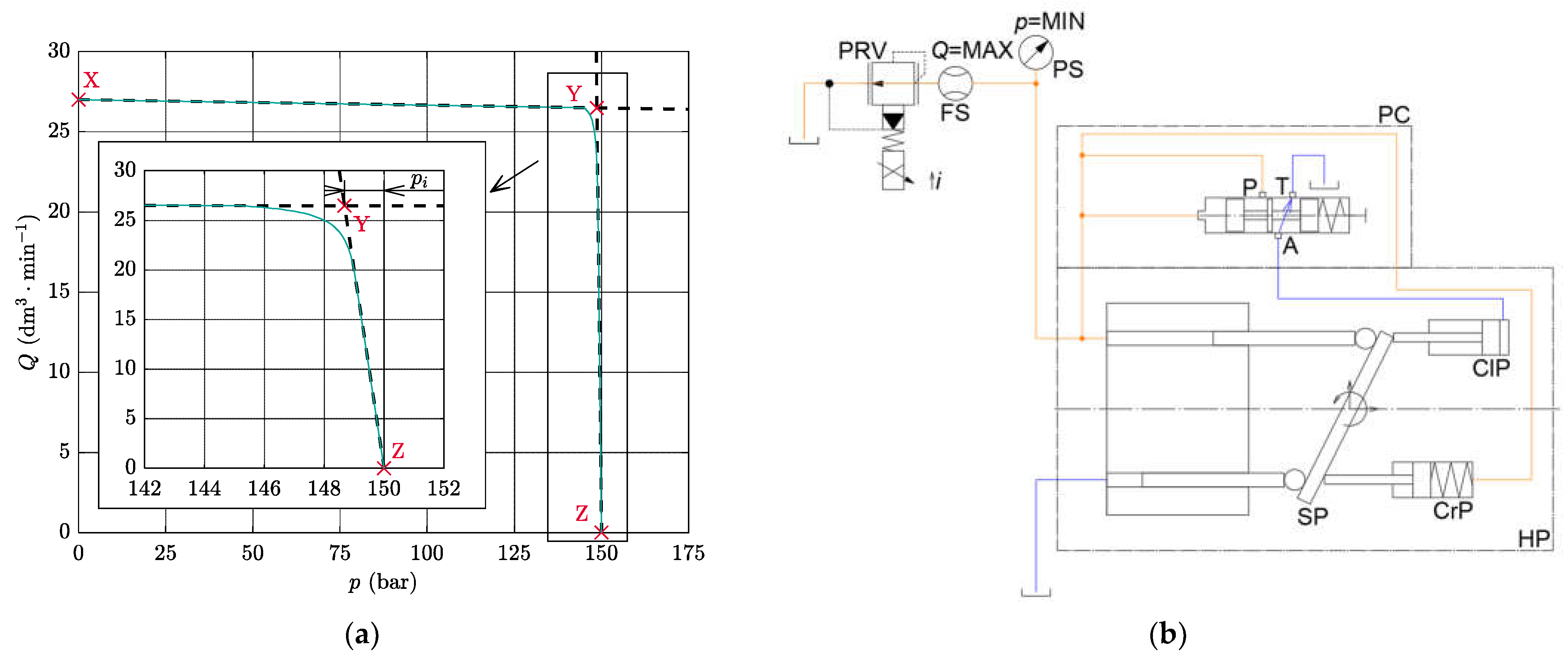
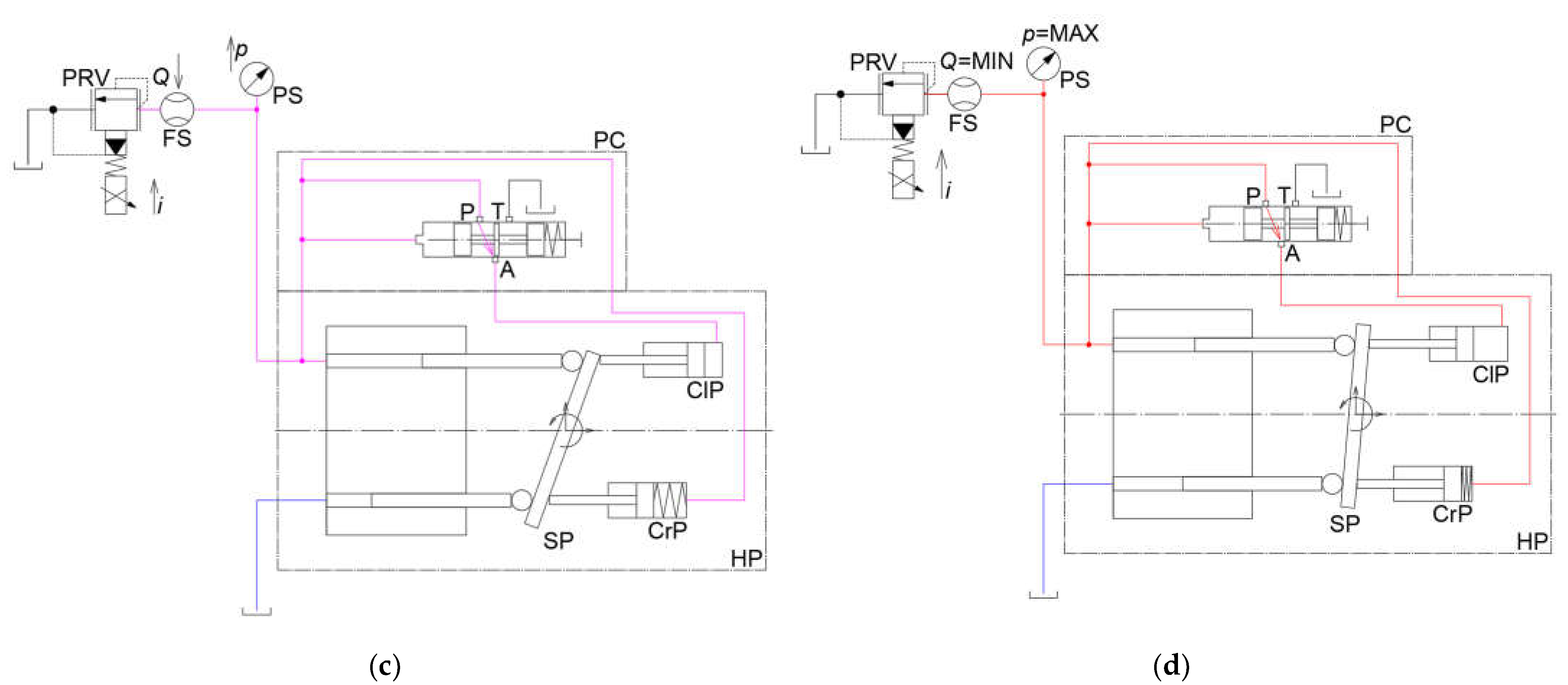
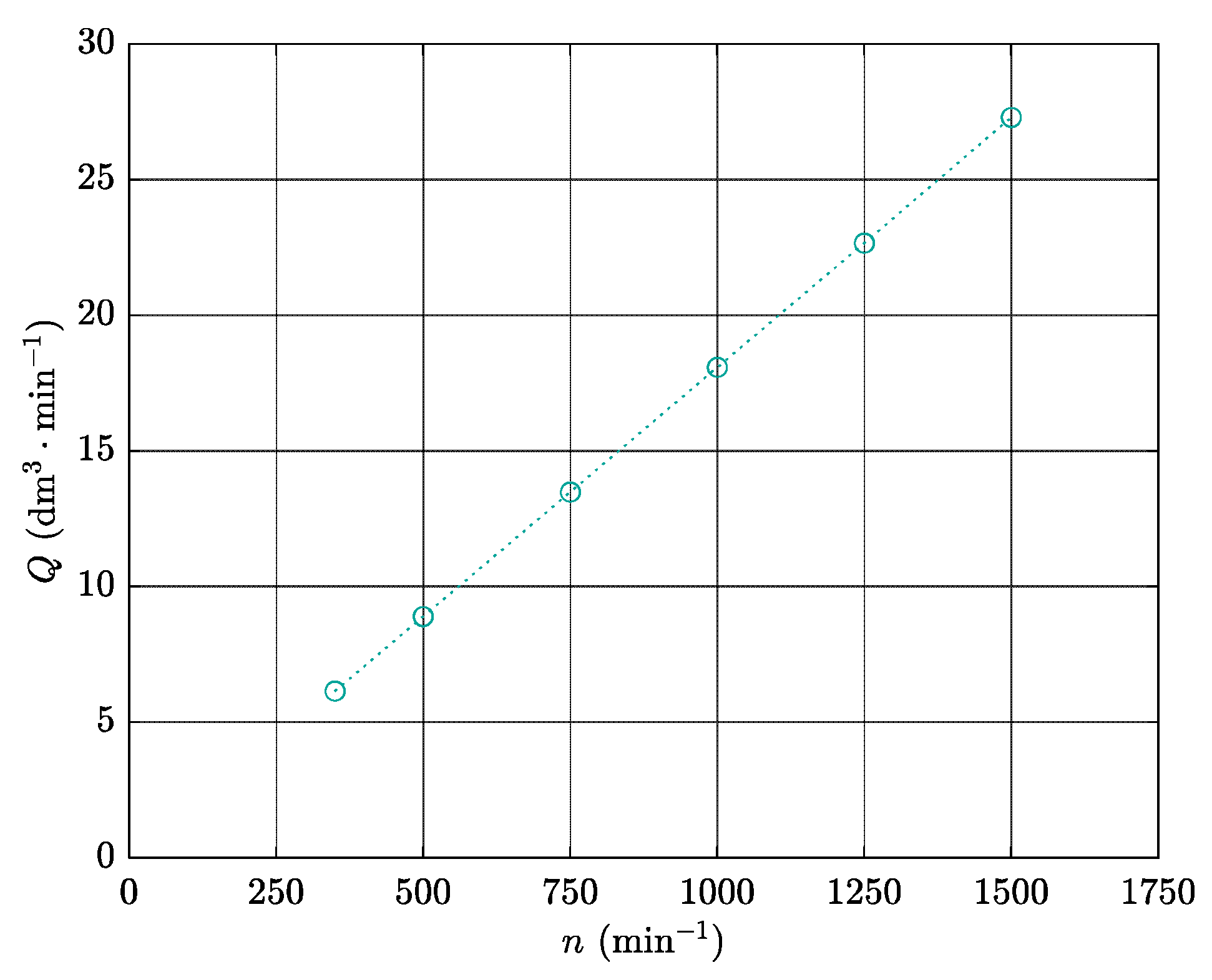
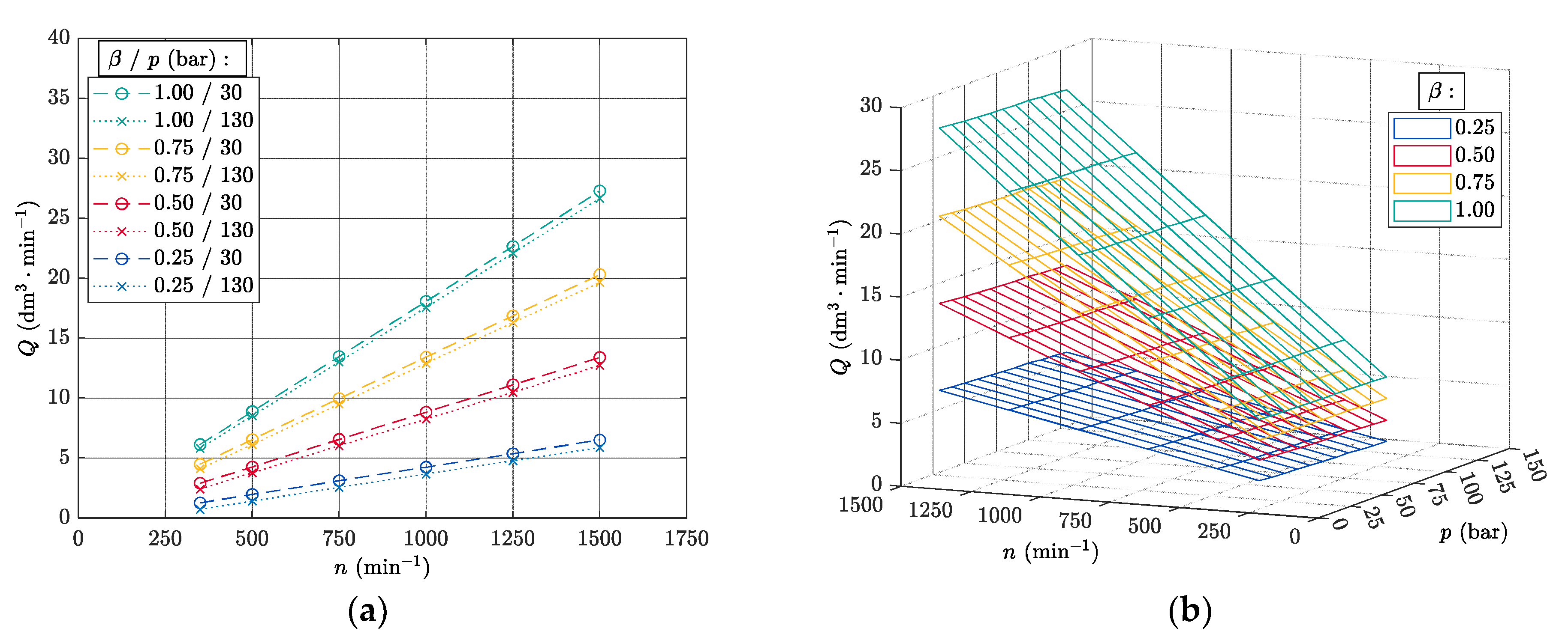
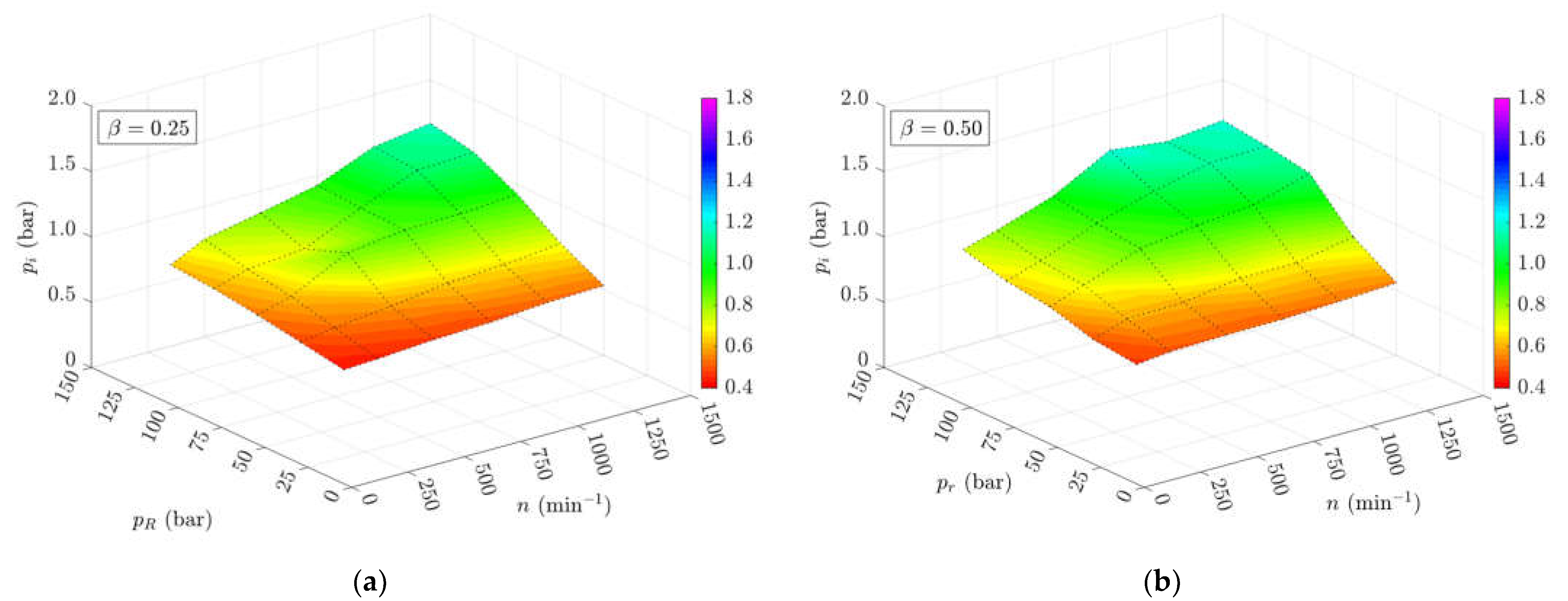
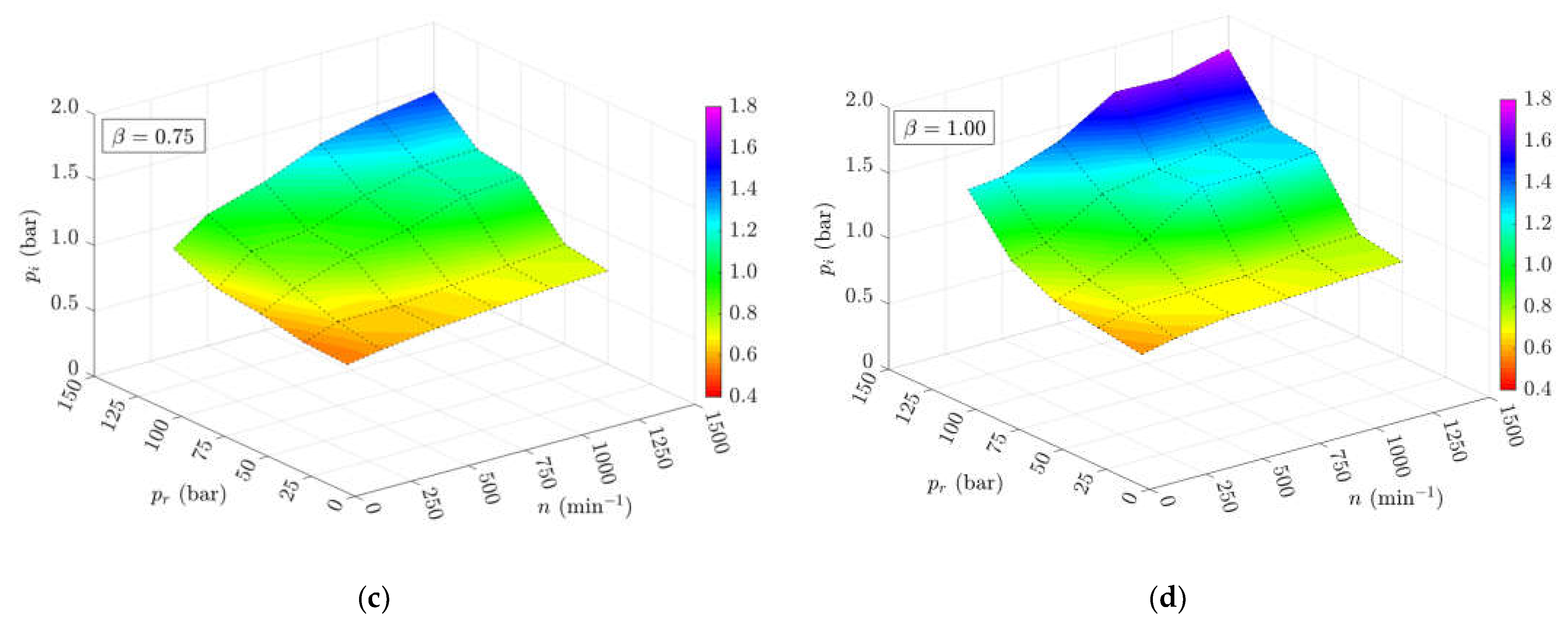
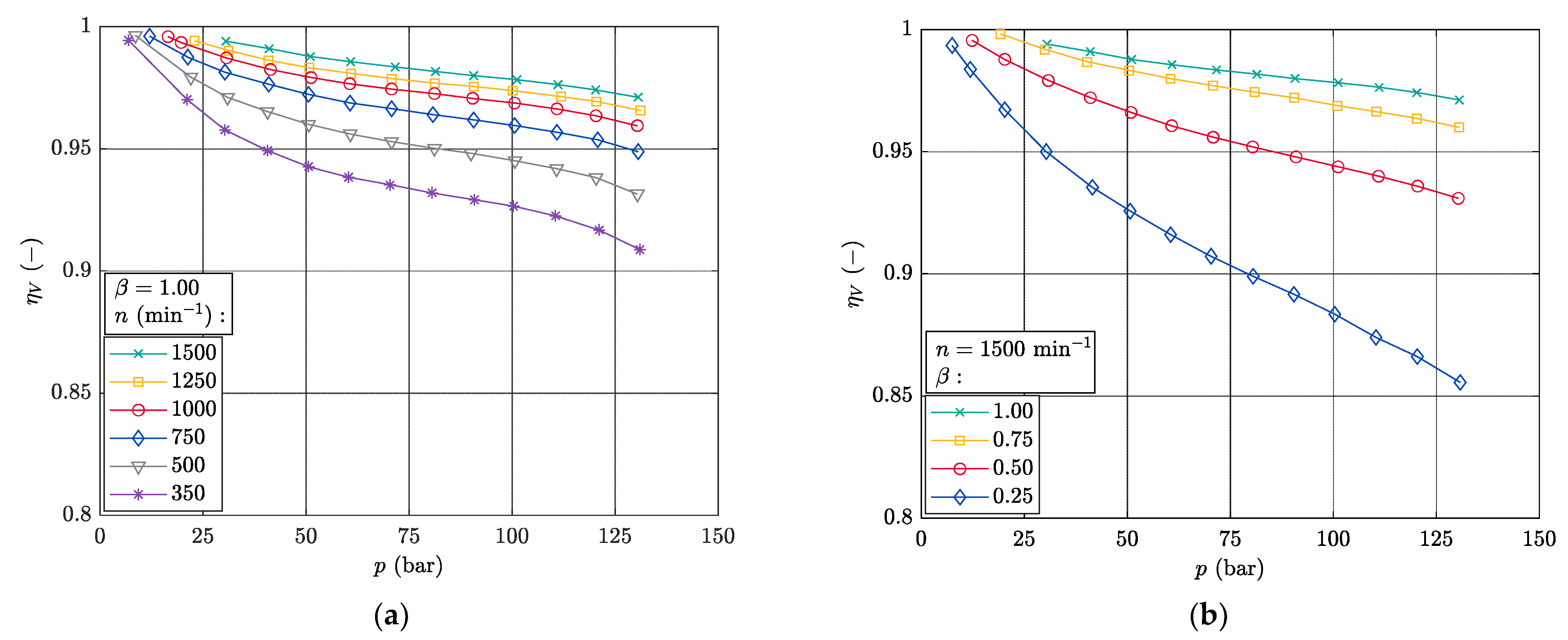
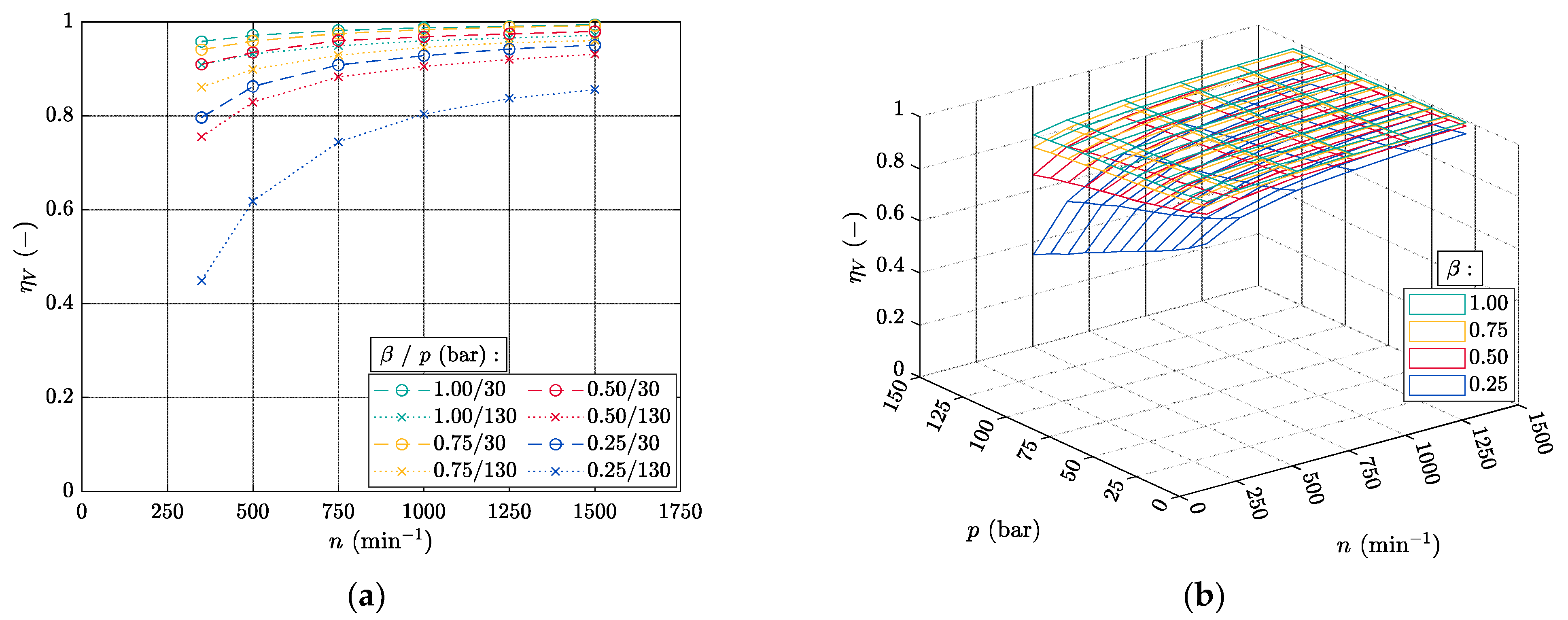
4.1. Flow Characteristics of the Pressure-Compensated Pump

The flow characteristic Q = f(p), as shown in Figure 6, represents the dependence of the pump flow rate Q on the pump outlet pressure p. These dependencies are determined for the different pump speeds n, different pressures p_PC set on the pressure compensator and different relative displacements β. These characteristics are mainly influenced by flow rate losses and pressure compensators.

Figure 6a shows that the pump flow rate Q decreases slightly with increasing pump outlet pressure p. This phenomenon is due to the loss of flow through the leakage of the pump. The leakage flow increases with increasing pressure. If the pump outlet pressure p approaches the pressure p_PC set at the pressure compensator, the pump displacement V_g decreases and so does the pump flow rate Q. It is also clear that as the pump speed n increases, the pump flow rate Q increases. In Figure 6b, it can be seen that the pump flow rate Q is regulated when the pump outlet pressure p approaches the pressure p_PC set at the pressure compensator. Subsequently, it can be seen, according to Figure 6c, that the flow Q increases with increasing relative displacement β.

Figure 6d shows that for a relative displacement β = 0.25 and pump speed n = (350; 500) min⁻¹, the pressure p_PC set at the pressure compensator is not achieved.

The flow characteristic Q = f(n), as shown in Figure 7a, represents the dependence of the pump flow rate Q on the pump speed n. These dependencies are determined for the relative displacements β = (1.00; 0.75; 0.50; 0.25) and the pump outlet pressures p = (30; 130) bar were chosen as the minimum and maximum pump outlet pressures achieved for all combinations of boundary conditions and are not biased by the displacement control. Figure 7b shows the complex flow characteristics for the different relative displacements β = (1.00; 0.75; 0.50; 0.25).

It is clear from these dependencies, as shown in Figure 7, that the interdependence of all the variables being compared is linear. The pump flow rate Q increases with increasing pump speed n and with increasing relative displacement β. Conversely, the pump flow rate Q decreases with increasing pump outlet pressure p.

From each flow characteristic curve Q = f(p), it is possible to define the pressure increase p_i. Pressure increase p_i indicates the regulation range of the pressure-compensated pump, as is explained in Figure 2a. The values of pressure increase p_i for each boundary condition are shown in

Table 3. Values of the pressure increase p_i for the different boundary conditions.

		β = 1.00						β = 0.75
	n (min−1)	350	500	750	1000	1250	1500	350	500	750	1000	1250	1500
pPC (bar)
50		0.56	0.62	0.67	0.69	0.71	0.73	0.54	0.58	0.63	0.67	0.70	0.71
75		0.61	0.69	0.70	0.70	0.78	0.79	0.55	0.64	0.64	0.69	0.72	0.77
100		0.66	0.76	0.94	1.23	1.23	1.27	0.62	0.74	0.88	0.96	1.10	1.14
125		0.82	0.89	1.14	1.21	1.27	1.31	0.66	0.88	0.92	1.06	1.17	1.18
150		1.21	1.24	1.39	1.65	1.64	1.75	0.81	1.00	1.13	1.31	1.41	1.47
		β = 0.50						β = 0.25
50		0.47	0.50	0.51	0.51	0.53	0.56	0.43	0.44	0.47	0.49	0.52	0.53
75		0.51	0.60	0.61	0.67	0.67	0.76	0.49	0.53	0.58	0.64	0.66	0.70
100		0.61	0.70	0.86	0.93	0.96	1.09	0.54	0.61	0.83	0.89	0.90	0.93
125		0.65	0.74	0.91	1.03	1.13	1.15	0.59	0.67	0.71	0.91	1.08	1.10
150		0.74	0.82	0.96	1.20	1.14	1.19	0.62	0.75	0.83	0.93	1.10	1.17

.

Figure 8 shows the pressure increase p_i according to the pressure p_PC set at the pressure compensator and the pump speed n for the relative displacements β. It can be seen from Figure 8 that the value of the pressure increase p_i increases with increasing pump speed n, the pressure increase p_i increases with increasing pressure p_PC set at the pressure compensator and also the pressure increase p_i increases with increasing relative displacement β.

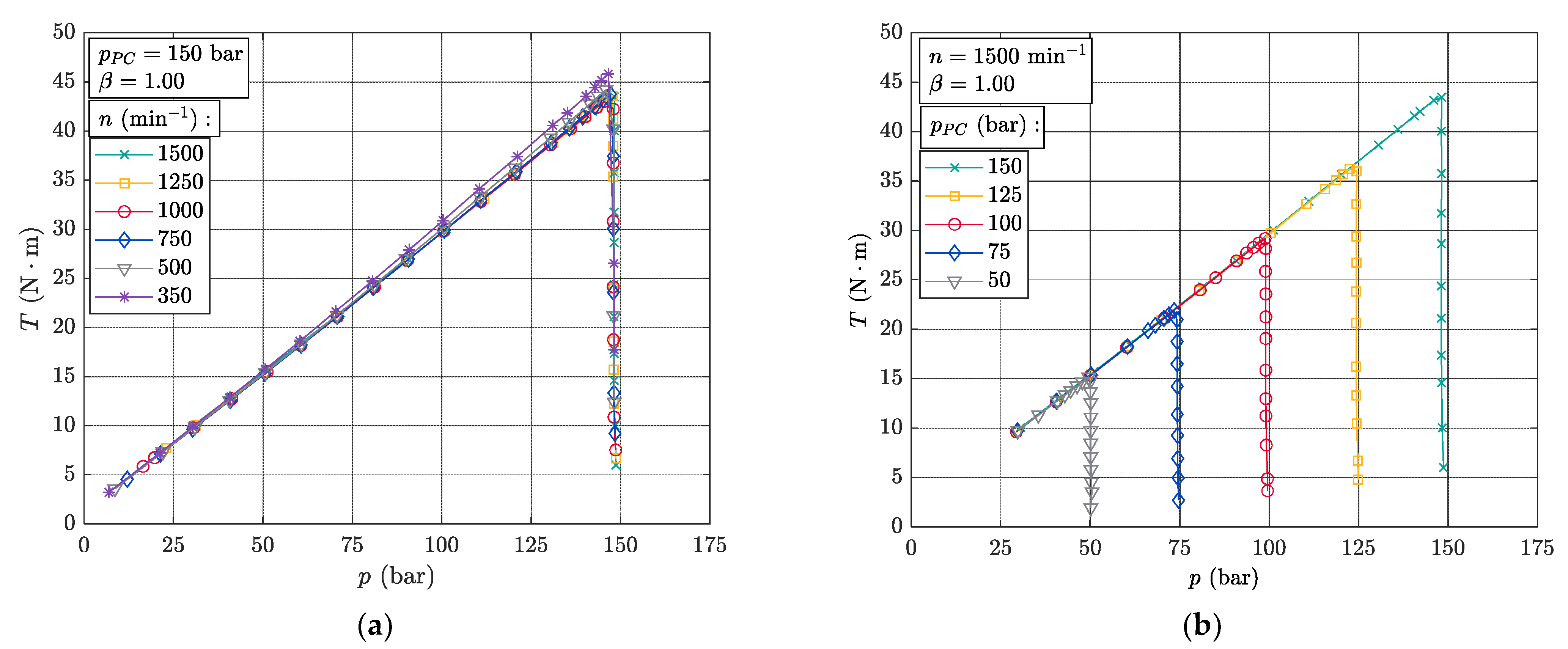
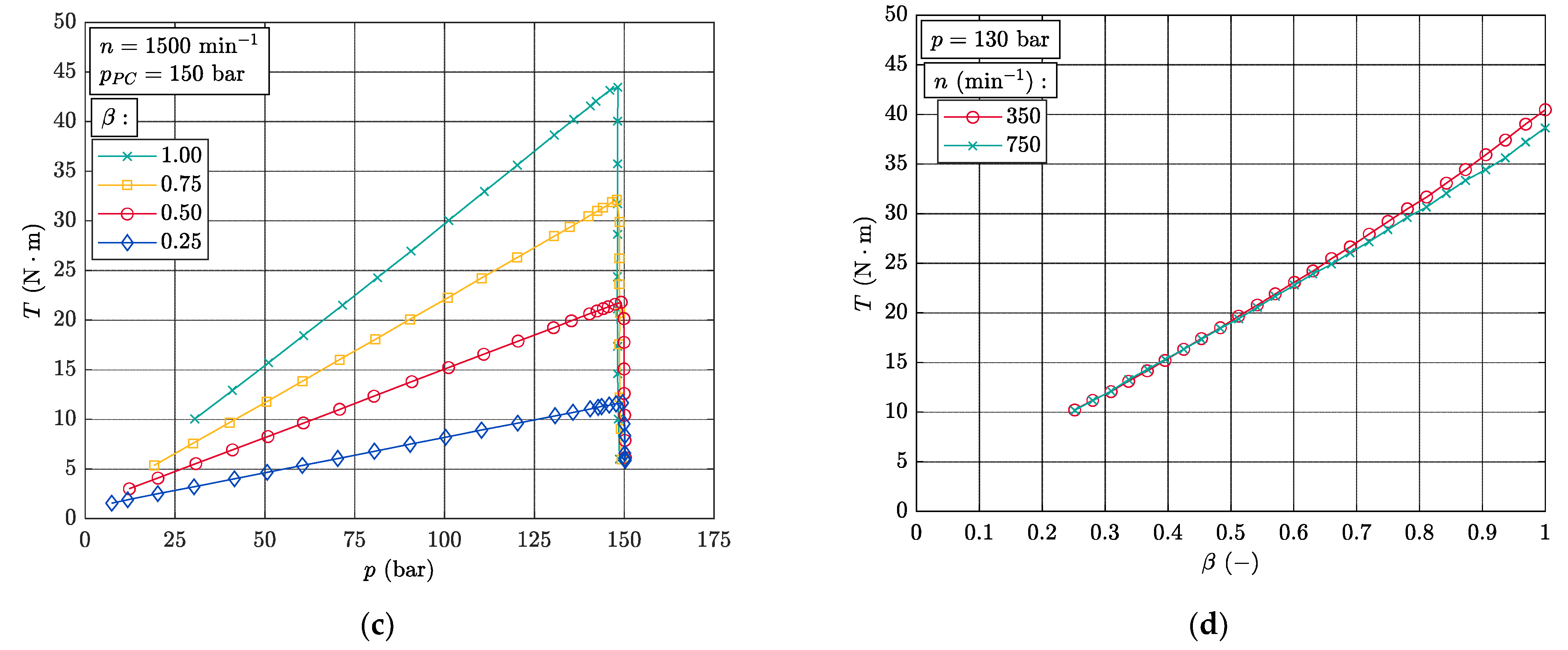
4.2. Torque Characteristic of the Pressure-Compensated Pump

The torque characteristic T = f(p), as shown in Figure 9a–c, represents the dependence of the torque T on the pump outlet pressure p. These dependencies are determined for the different pump speeds n, for the different pressures p_PC set at the pressure compensator and for the different relative displacements β. Figure 9d shows the dependence of the torque T on the relative displacement β for the pump speed n = (350; 750) min⁻¹.

Figure 9 shows that the torque T increases with increasing pump outlet pressure p to the point given by the pressure p_PC set at the pressure compensator. Consequently, the torque T decreases together with the decreasing pump displacement V_g. In Figure 9a, it can be noticed that in the zone outside the displacement control, the torque is independent of the pump speed n for the speed range n = (1500; 1250; 1000; 750) min⁻¹. In the case of speed n = (500; 350) min⁻¹, there is a deviation from the trend with increasing pump outlet pressure p. This is due to the increase in the passive resistances for low speed n. In Figure 9b, it can be seen that the torque T starts to decrease along with the decrease in the pump displacements V_g when the pressure p_PC set at the pressure compensator is reached. Figure 9c shows that for constant pump outlet pressure p, the torque T increases with increasing relative displacement β. In Figure 9d, it can be seen that the deviation from the trend occurs only for higher relative displacements β for lower pump speeds n. As the relative displacement β decreases, both trends merge. Based on this dependence, it can be concluded that in the case of pure speed control, passive resistances increase and mechanical pressure efficiency decreases for pump speeds lower than n = 500 min⁻¹. If speed control and displacement control are used simultaneously, the increase in the passive resistances for lower pump speed n does not occur. As the pump speed decreases, the lubrication between the Individual parts of the pump deteriorates and this results In increasing friction between these parts [25,26].

Figure 10a shows the dependence of the torque T on the pump speed n for the relative displacements β = (1.00; 0.75; 0.50; 0.25) and for the pump outlet pressures p = (30; 130) bar. Figure 10b shows the complex dependence of the torque T on the pump speed n and the pump outlet pressure p for the relative displacements β = (1.00; 0.75; 0.50; 0.25).

In Figure 10, it can be seen that the torque T is almost independent of the pump speed n in the measured range. In the case of the relative displacement β = (1.00; 0.75), it can be seen that for lower speed n < 500 min⁻¹, there is an increase in torque T. This increase is due to the higher passive resistances for the low pump speeds n and the higher relative displacements β. At low pump speeds, there is inadequate lubrication of the individual pump parts, which increases friction between these parts. The increase in torque T is more noticeable for the higher pump outlet pressure p when higher forces are applied to the bearings. It can also be noticed that the torque T increases with increasing relative displacement β and increasing pump outlet pressure p. Figure 10b shows that there can be a higher torque increase in the low pump speed range due to increased friction caused by insufficient lubrication between individual pump parts. It can also be seen that torque increases with increasing pump outlet pressure.

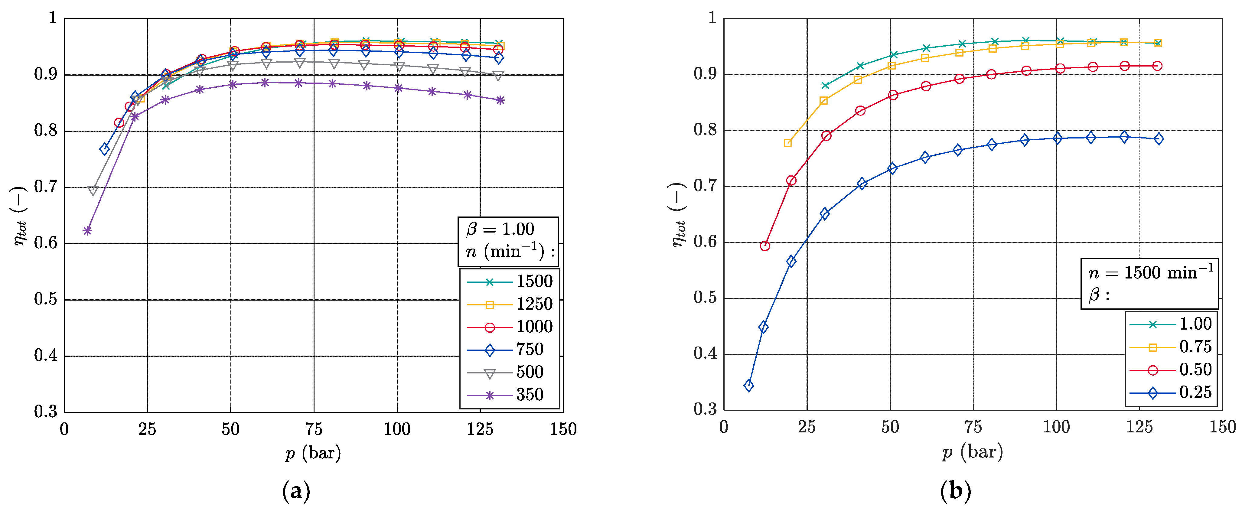
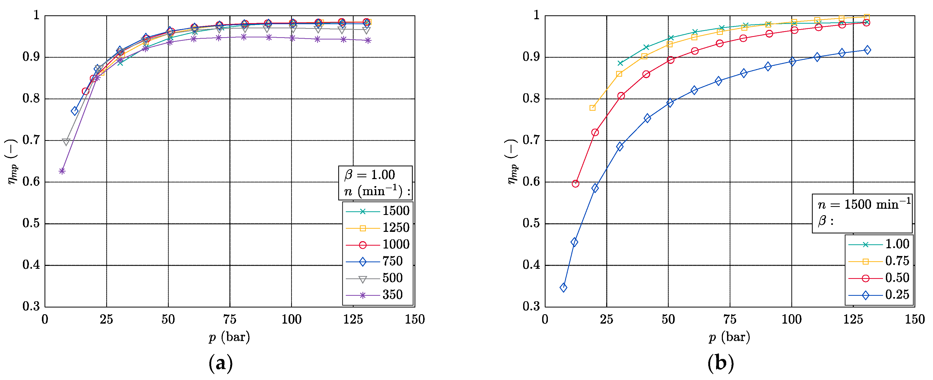
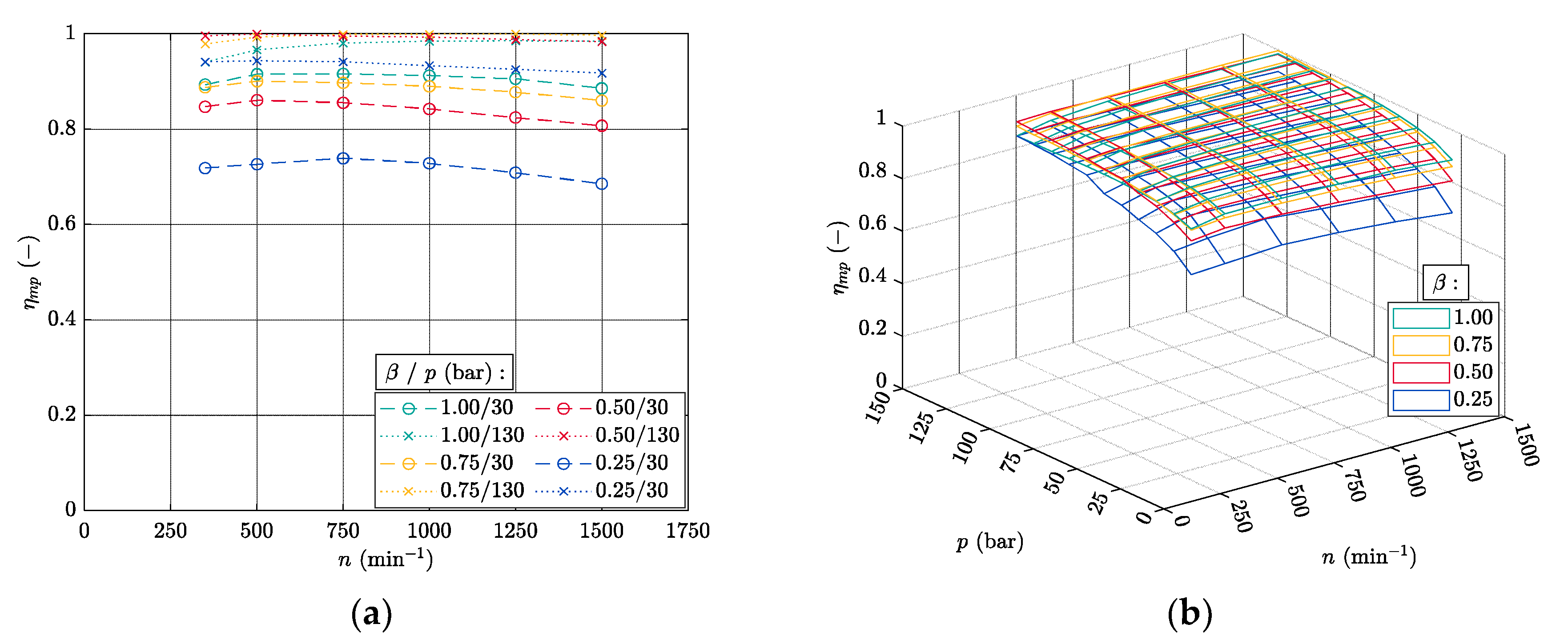
4.3. Efficiency of the Pressure-Compensated Pump

From the measurements taken, the total efficiency η_tot, the volumetric efficiency η_V and mechanical pressure efficiency η_mp were determined. Figure 11a shows the dependence of the total efficiency η_tot on the pump outlet pressure p for the different pump speeds n and Figure 11b shows the dependence of the total efficiency η_tot on the pump outlet pressure p for the different relative displacements β.

The results, as shown in Figure 11, show that as the pump outlet pressure p increases, the total efficiency η_tot first increases and then slightly decreases. From Figure 11b, it can be seen that as the relative displacement β increases, the total efficiency η_tot increases over the entire range of measured pump outlet pressure p.

Next, the total efficiency η_tot was evaluated according to pump speed n for the relative displacements β = (1.00; 0.75; 0.50; 0.25) and the pump outlet pressures p = (30; 130) bar (see Figure 12a). Figure 12b shows the complex dependence of the total efficiency η_tot on the pump speed n and the pump outlet pressure p.

In Figure 12a, it can be seen that for the relative displacements β = (1.00; 0.75) and for the pump outlet pressure p = 130 bar, all the dependencies have an increasing tendency. In the case of the pump outlet pressure p = 30 bar, the total efficiency η_tot first increases with increasing pump speed n and then decreases after exceeding the pump speed value n = 750 min⁻¹. Furthermore, it is evident that lower relative displacements β = (0.50; 0.25) have a significant effect on the total efficiency η_tot, whereas the relative displacement β decreases, and there is a non-linear decrease in the total efficiency η_tot over the entire measured pump speed n range.

Furthermore, the volumetric efficiency η_V was evaluated according to the pump outlet pressure p, for the different pump speeds n (see Figure 13a) and for the different relative displacements β (see Figure 13b).

The results in Figure 13 show that the volumetric efficiency η_V decreases with increasing pump outlet pressure p. From Figure 13b, it can be seen that the relative displacement β has a significant effect on the volumetric efficiency η_V and as the relative displacement β, the volumetric efficiency η_V decreases over the entire range of measured pump outlet pressures p.

This is due to the design of the swash plate mounting, where the swash axis of the plate is located in the plane of the hydraulic shaft axis. Thus, the dead volume is larger at lower values of the relative displacement β. In the case of a larger dead volume, the flow rate into the hydraulic capacity of the piston working space is larger. This results in a drop in the flow rate at the pump outlet. The flow rate to the hydraulic capacity of the dead volume then expands back into the pump inlet. The higher the dead volume is, the lower the volumetric efficiency [28,29].

Next, the volumetric efficiency η_V was evaluated according to the pump speed n for the relative displacement β = (1.00; 0.75; 0.50; 0.25) and for the pump outlet pressures p = (30; 130) bar (see Figure 14a). Figure 14b shows the complex dependence of the volumetric efficiency η_V on the pump speed n and on the pump outlet pressure p.

In Figure 14a, it can be seen that the volumetric efficiency η_V increases with increasing pump speed n. It can also be seen that the volumetric efficiency η_V increases with increasing relative displacement β and conversely decreases with increasing pump outlet pressure p. Figure 14b confirms that the volumetric efficiency η_V decreases with increasing pump outlet pressure p and increases with increasing pump speed n. It is also confirmed that the volumetric efficiency η_V increases with increasing relative displacement β.

Next, the mechanical pressure efficiency η_mp was evaluated according to the pump outlet pressure p, for the different pump speeds n (see Figure 15a), and for the different relative displacements β (see Figure 15b).

The results in Figure 15 show that the mechanical pressure efficiency η_mp increases with increasing pump outlet pressure p. From Figure 15b, it can be seen as the relative displacement β the mechanical pressure efficiency η_mp increases. In the case of the trend determined by the relative displacement β = 1.00, a crossover of the trend for the relative displacement β = 0.75 occurs for the pump outlet pressure of about p = 100 bar.

Next, the mechanical pressure efficiency η_mp was evaluated according to the pump speed n for the relative displacement β = (1.00; 0.75; 0.50; 0.25) and the pump outlet pressures p = (30; 130) bar (see Figure 16a). Figure 16b shows the complex dependence of the mechanical pressure efficiency η_mp on the pump speed n and the pump outlet pressure p for the different relative displacements β.

In Figure 16a, it can be seen that the mechanical pressure efficiency η_mp first increases and then decreases with increasing pump speed n.

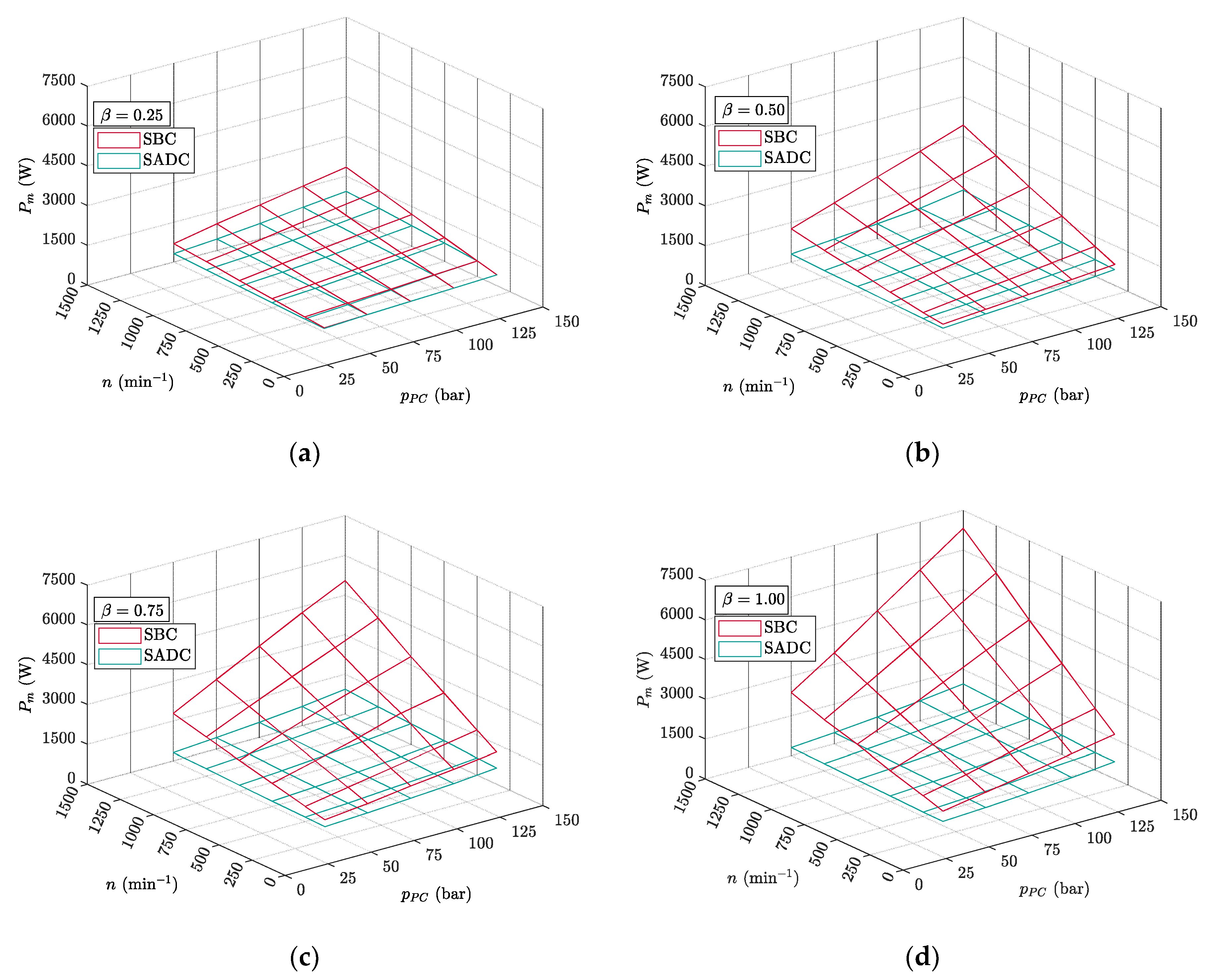
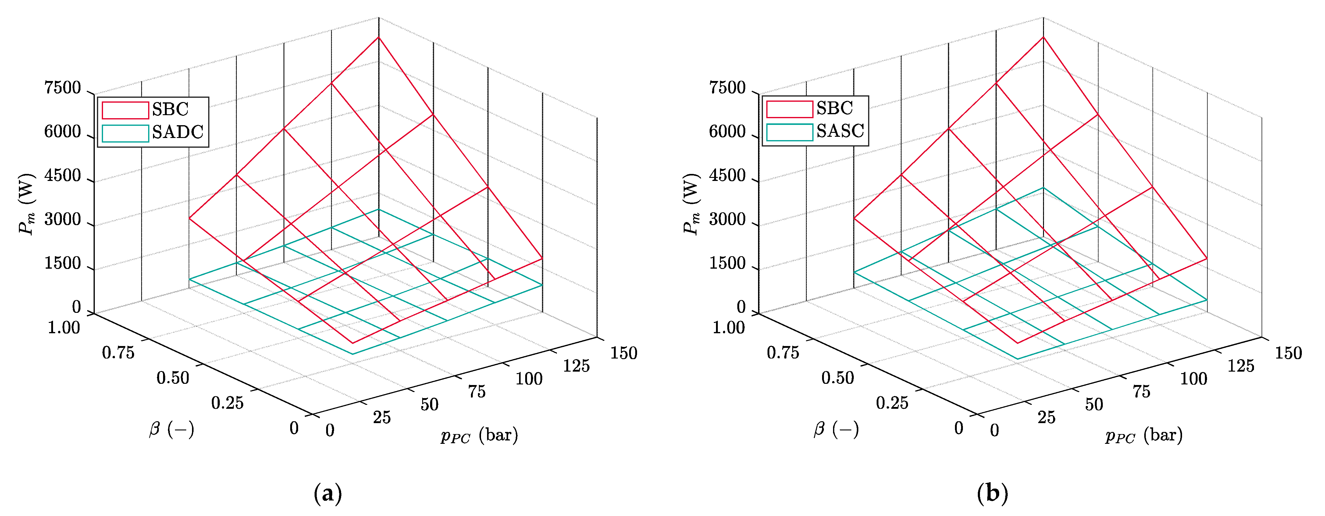
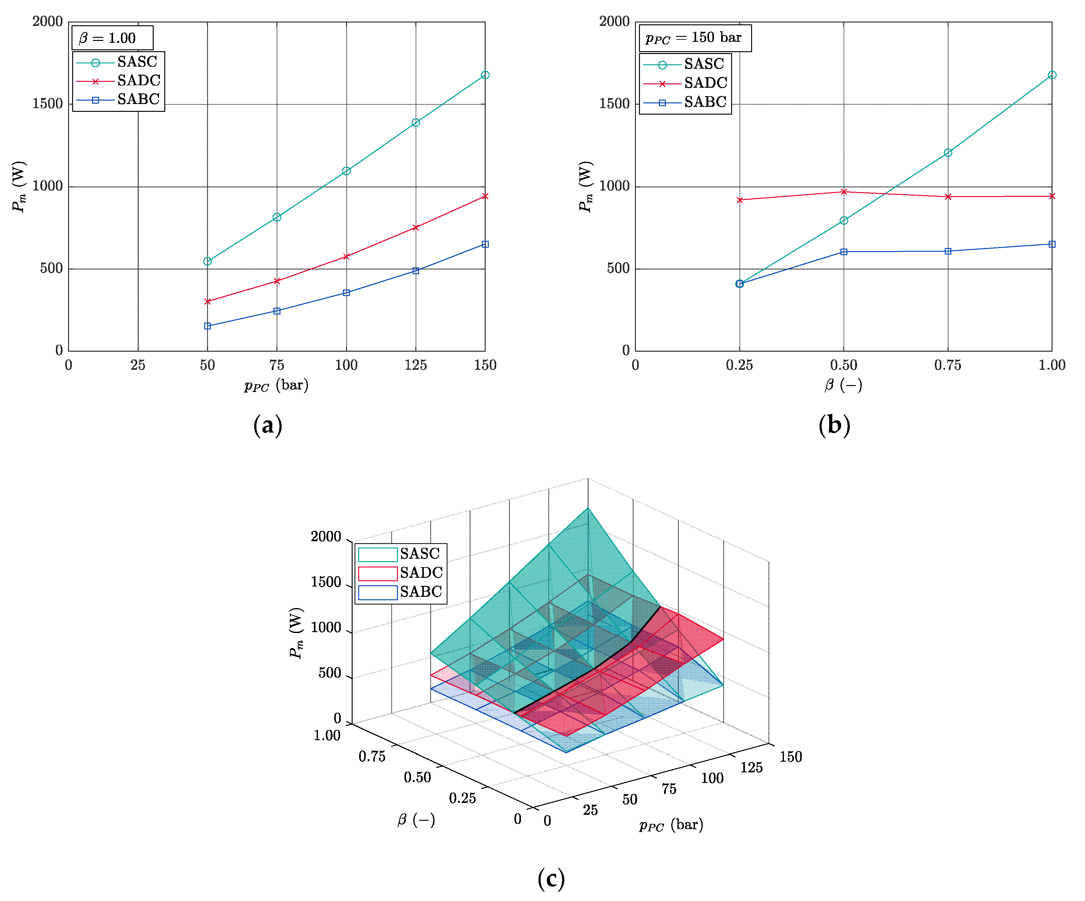
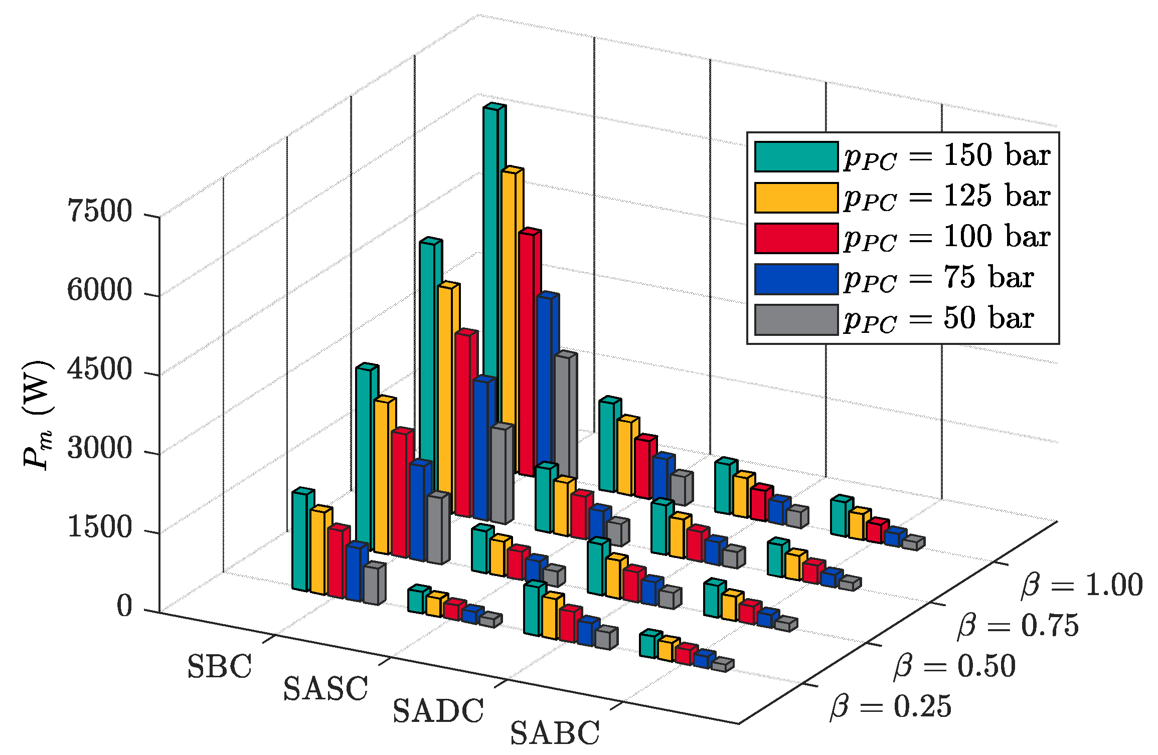
4.4. Comparison of the Stand-by Mechanical Input Power

The mechanical input power P_m of the pump was chosen as a variable for comparison of the individual control methods. The mechanical input power P_m is determined at the shaft of the pump from the measured pump speed n and the torque T according to Equation (7).

Table 4. Individual states of control.

Label	State Description
SBC	The state before control
SADC	The state after displacement control
SASC	The state after speed control
SABC	The state after both controls

shows explanations of the individual control states.

Figure 17 shows the comparisons of the mechanical input power P_m for the state before control (SBC) and for the state after displacement control (SADC) for the different pump speeds n, pressures p_PC set at the pressure compensator and the relative displacements β.

In Figure 17, it can be seen that the mechanical input power P_m for the state before control (SBC) and for the state after displacement control (SADC) increases with increasing pump speed n and also increases with increasing pressure p_PC set at the pressure compensator. By comparing the dependencies for each relative displacement β, it can be seen that for the state before control (SBC), the mechanical input power P_m increases with increasing relative displacement β. The mechanical input power P_m for the state after displacement control (SADC) is the same for the measured relative displacement β = (1.00; 0.75; 0.50; 0.25) because the minimum pump displacement V_gmin is smaller than the relative displacement β = 0.25.

Next, a comparison is conducted between the maximum input power and input power for the state before control (SBC) and the state after displacement control (SADC), as shown in Figure 18a, and for the state before control (SBC) and the state after speed control (SASC), as shown in Figure 18b. These input powers are evaluated for the different relative displacement β and for the different pressures p_PC set at the pressure compensator. From Figure 18, it can be seen in the case of the speed control, the input power for the minimum pump speed n_min is more dependent on the pressure p_PC set at the pressure compensator than in the case of displacement control. It can also be seen that in the case of displacement control, the input power P_m is not dependent on the relative displacement, unlike in the case of speed control (see Figure 18b).

It can be seen from Figure 18 that for both control methods, the highest power saving is achieved for the maximum relative displacement β and for the highest pressure p_PC set at the pressure compensator. As the relative displacement β decreases and the pressure p_PC set at the pressure compensator decreases, the mechanical input power P_m decreases and the power saving also decreases. Power saving determines how the mechanical input power P_m is reduced between the working state (the state before control—SBC) and the stand-by state (state after displacement control—SADC, state after speed control—SASC or state after both controls—SABC).

Figure 19 compares the mechanical input power P_m after the speed control (SASC), after the displacement control (SADC) and after both controls simultaneously (SABC). These input power P_m are evaluated for the different relative displacements β (see Figure 19b) and for the different pressures p_PC set at the pressure compensator (see Figure 19a).

With an increasing pressure p_PC set at the pressure compensator, the input power increases (see Figure 19a). Decreasing the relative displacement β affects the power saving only when the speed control occurs, see Figure 19b. It can be noticed that the most energy-saving solution is to use a combination of both control methods.

Furthermore, it was evaluated by what percentage the mechanical input power P_m is reduced during the displacement control (SADC), i.e., the pump displacement is reduced from the actual maximum value of the pump displacement V_gset to the minimum value of the pump displacement V_gmin. It was also evaluated by what percentage the mechanical input power P_m is reduced during the speed control (SASC) when the pump speed n is reduced from n = 1500 min⁻¹ to n = 350 min⁻¹. Finally, it was evaluated by what percentage the mechanical input power P_m is reduced during both controls (SABC). These data are shown in

Table 5. Percentage mechanical input power saving for the displacement control, the speed control and both controls.

		Displacement Control					Speed Control					Both Controls
	pPC (bar)	150	125	100	75	50	150	125	100	75	50	150	125	100	75	50
β (-)
1.00		86.2	86.8	87.5	87.6	87.4	75.4	75.6	76.1	76.4	77.1	90.5	91.4	92.3	92.9	93.6
0.75		81.4	82.8	83.6	83.6	82.6	76.1	76.5	76.5	77.2	76.6	87.9	89.1	89.9	91.0	91.6
0.50		71.7	74.9	75.7	75.5	75.6	76.8	77.0	77.2	76.9	77.1	82.4	84.0	85.5	86.5	88.2
0.25		49.9	51.2	54.2	57.0	53.7	77.7	77.6	77.8	78.0	77.8	77.7	77.6	77.8	78.0	80.2

.

It can be seen from the percentage of mechanical input power savings shown in Table 5 that for the maximum relative displacement β = 1.00, the power saving for the displacement control is higher than for the speed control. For the relative displacement β = 0.50, the power saving for the displacement control and the speed control are similar. For the case of relative displacement β = 0.25, it can be noticed that the power saving is higher for the speed control. For the case of both control methods, the effect of speed control on the total power saving increases with decreasing the pressure p_PC set at the pressure compensator and decreasing the relative displacement β. The total power saving is in the interval (77.6–93.6%). The maximum power saving is for the maximum relative displacement β = 1.00.

Figure 20 confirms that as the relative displacement β decreases, the speed control has a greater effect on the power saving.

5. Conclusions

The aim of the study is to determine the static characteristics and energy consumption of the pressure-compensated pump. In order to determine the above characteristics of the pump, an experimental device was assembled. This device allows us to change individual boundary conditions and measures the necessary variables. Based on the measurements, the flow characteristics, torque characteristics and individual efficiencies for the different boundary conditions were evaluated. The boundary conditions that were set are the pump speed, the pump outlet pressure, the pressure set at the pressure compensator and the relative displacement. Furthermore, the pressure increase was evaluated. Another motivation for this study was to verify the possibilities of saving input power in a stand-by state with different methods of constant pressure control. A stand-by state corresponds to a condition where there is no system flow rate requirement. In the stand-by state, the pump maintains a set constant pressure. The main contributions of this work include the following:

• The individual static characteristics and dependencies of the monitored variables in a wide range of boundary conditions were measured and determined.
• It was found that with the maximum relative displacement and higher values of the pressure at the pump outlet pressure, there is a deviation from the linear trend of the torque according to the pump speed. A significant deviation occurs for the lower speeds (n < 500 min⁻¹). This is due to the higher passive resistances when the swash plate is tilted at the greatest swash angle and the radial forces reach the highest values. From these findings, it can be concluded that for the speed n < 500 min⁻¹, more stresses occur and this pump should not be operated below these critical pump speeds for a long time.
• Power savings were evaluated for the displacement control, the speed control and both control methods simultaneously. From the results obtained, it is clear that the displacement control has a more significant effect on the power saving of the pump in a wider range of boundary conditions. Speed control is generally preferable for the smaller relative displacements where the swash plate is tilted at a lower angle. Using both controls simultaneously brings the greatest total input power savings.

This paper presents a comprehensive set of measured and determined static characteristics of the axial piston pressure-compensated pump. These characteristics can be used in particular to compare different types of pumps or to determine the suitability of a pump for a particular application. These characteristics can also be used to verify the mathematical model of the pressure-compensated pump. Further research will be directed to the dynamics of individual control methods.

References

1. Kim, J.-H.; Jeon, C.-S.; Hong, Y.-S. Constant Pressure Control of a Swash Plate Type Axial Piston Pump by Varying Both Volumetric Displacement and Shaft Speed. Int. J. Precis. Eng. Manuf. 2015, 16, 2395–2401. [Google Scholar] [CrossRef]
2. Yan, Z.; Ge, L.; Quan, L. Energy-Efficient Electro-Hydraulic Power Source Driven by Variable-Speed Motor. Energies 2022, 15, 4804. [Google Scholar] [CrossRef]
3. Yang, X.; Gong, G.; Yang, H.; Jia, L.; Zhou, J. An Investigation in Performance of a Variable-Speed-Displacement Pump-Controlled Motor System. IEEE/ASME Trans. Mechatron. 2017, 22, 647–656. [Google Scholar] [CrossRef]
4. Ge, L.; Quan, L.; Zhang, X.; Dong, Z.; Yang, J. Power Matching and Energy Efficiency Improvement of Hydraulic Excavator Driven with Speed and Displacement Variable Power Source. Chin. J. Mech. Eng. 2019, 32, 100. [Google Scholar] [CrossRef]
5. Kauranne, H. Effect of Operating Parameters on Efficiency of Swash-Plate Type Axial Piston Pump. Energies 2022, 15, 4030. [Google Scholar] [CrossRef]
6. Fornarelli, F.; Lippolis, A.; Oresta, P.; Posa, A. A computational model of axial piston swashplate pumps. In Proceedings of the 72nd Conference of the Italian Thermal Machines Engineering Association, Lecce, Italy, 6–8 September 2017. [Google Scholar]
7. Xu, B.; Hu, M.; Zhang, J.; Su, Q. Characteristics of volumetric losses and efficiency of axial piston pump with respect to displacement conditions. J. Zhejiang Univ. Sci. A 2016, 3, 186–201. [Google Scholar] [CrossRef]
8. Xu, B.; Hu, M.; Zhang, J.; Mao, Z. Distribution characteristics and impact on pump’s efficiency of hydro-mechanical losses of axial piston pump over wide operating ranges. J. Cent. S. Univ. 2017, 24, 609–624. [Google Scholar] [CrossRef]
9. Hasko, D.; Shang, L.; Noppe, E.; Lefrançois, E. Virtual Assessment and Experimental Validation of Power Loss Contributions in Swash Plate Type Axial Piston Pumps. Energies 2019, 12, 3096. [Google Scholar] [CrossRef]
10. Li, Y.; Yu, C.; Chen, G.; Yang, M.; Zhang, Y.; Wang, F. An Electro-Hydraulic-Load-Sensitive System on the Basis of Torque Open-Loop Control. Processes 2023, 11, 2618. [Google Scholar] [CrossRef]
11. Kardoub, M.A.; Gad, O.E.; Rabie, M.G. Predicting Axial Piston Pump Performance Using Neural Networks; Elsevier Science Ltd.: Amsterdam, The Netherlands, 1998. [Google Scholar]
12. Zardin, B.; Natali, E.; Borghi, M. Evaluation of the Hydro-Mechanical Efficiency of External Gear Pumps. Energies 2019, 12, 2468. [Google Scholar] [CrossRef]
13. Chiavola, O.; Frattini, E.; Palmieri, F.; Fiovanti, A.; Marani, P. On the Efficiency of Mobile Hydraulic Power Packs Operating with New and Aged Eco-Friendly Fluids. Energies 2023, 16, 5681. [Google Scholar] [CrossRef]
14. Zhang, C.; Ruan, J.; Xing, T.; Li, S.; Meng, B.; Ding, C. Research on the Volumetric Efficiency of a Novel Stacked Roller 2D Piston Pump. Machines 2021, 9, 128. [Google Scholar] [CrossRef]
15. Osiński, P.; Deptuła, A.; Partyka, M.A. Hydraulic Tests of the PZ0 Gear Micropump and the Importance Rank of Its Design and Operating Parameters. Energies 2022, 15, 3068. [Google Scholar] [CrossRef]
16. Osiński, P.; Deptuła, A.; Partyka, M.A. Discrete optimization of a gear pump after tooth root undercating by means of multi-valuated logic trees. Arch. Civ. Mech. Eng. 2013, 13, 422–431. [Google Scholar] [CrossRef]
17. Bergada, J.M.; Kumar, S.; Davies, D.L.; Watton, J. A complete analysis of axial piston pump leakage and output flow ripples. Appl. Math. Model. 2012, 36, 1731–1751. [Google Scholar] [CrossRef]
18. Hujo, Ľ.; Noasin, J.; Borowski, S.; Markiewicz-Palaton, M.; Tomić, M.; Kožuch, P. Design of a Laboratory Test Equipment for Measuring and Testing Mobile Energy Means with Simulation of Operating Conditions. Processes 2022, 10, 1435. [Google Scholar] [CrossRef]
19. Novak, N.; Trajkovski, A.; Kalin, M.; Majdič, F. Degradation of Hydraulic System due to Wear Particles or Medium Test Dust. Appl. Sci. 2023, 13, 7777. [Google Scholar] [CrossRef]
20. Kolodin, I.; Ryabinin, M. Mathematical representation of pressure regulator with variable characteristic. In IOP Conference Series: Materials Science and Engineering; IOP Publishing: Bristol, UK, 2019; Volume 589. [Google Scholar]
21. Burennikov, Y. Design Optimization of the Flow Rate Regulator for Axial-Plunger LS Pump Using LP Search Method. In Proceedings of the 17th International Conference TEHNOMUS—New Technologies and Products in Machine Manufacturing Technologies, Suceava, Romania, 17–18 May 2013. [Google Scholar]
22. Ma, H.; Liu, W.; Wu, D.; Shan, H.; Xia, S.; Xia, Y. Modelind and analysis of the leakage performance of the spherical valve plate pair in axial piston pumps. Eng. Sci. Technol. 2023, 45, 101498. [Google Scholar]
23. Bureček, A.; Hružík, L.; Vašina, M. Determination of Undissolved Air Content in Oil by Means of a Compression Method. Stroj. Vestn. J. Mech. Eng. 2015, 61, 447–485. [Google Scholar] [CrossRef]
24. Załuski, P. Experimental research of an axial piston pump with displaced swash plate axis of rotation. In International Scietific-Technical Conference on Hydraulic and Pneumatic Drives and Control; Springer: Berlin/Heidelberg, Germany, 2020; pp. 135–145. [Google Scholar]
25. Zhu, Y.; Chen, X.; Zou, J.; Yang, H. A study on the influence of surface topography on the low-speed tribological performance of ports plates in axial piston pumps. Wear 2015, 338–339, 406–417. [Google Scholar] [CrossRef]
26. Hong, Y.S.; Lee, S.Y. A Comparative Study of Cr-X-N (X=Zr, Si) Coatings for the Improvement of the Low-Speed Torque Efficiency of a Hydraulic Piston Pump. Met. Mater. Int. 2008, 14, 33–40. [Google Scholar]
27. Jeong, H.-S.; Kim, H.-E. On the Instantaneous and average Piston Friction of Swash Plate Type Hydraulic Axial Piston Machines. KSME Int. J. 2004, 18, 1700–1711. [Google Scholar] [CrossRef]
28. Chao, Q.; Xu, Z.; Tao, J.; Liu, C. Capped piston: A promising design to reduce compressibility effects, pressure ripple and cavitation for high-speed and high- pressure axial piston pumps. Alex. Eng. J. 2023, 62, 509–521. [Google Scholar] [CrossRef]
29. Załuski, P. Influence of Fluid Compressibility and Movements of the Swash Plate Axis of Rotation on the volumetric Efficiency of Axial Piston Pumps. Energies 2022, 15, 298. [Google Scholar] [CrossRef]
Figure 1. Individual parts of the pressure-compensated pump: (a) main components, (b) control mechanism of the swash plate, (c) main parts of the pump, (d) pressure compensator.
Processes 12 01081 g001
Figure 2. Illustration of individual states of pressure-compensated pump: (a) flow characteristic with indication of pressure increase, (b) schematic illustration of control state for X-Y zone, (c) schematic illustration of control state for Y-Z zone, (d) schematic illustration of control state for point Z.
Processes 12 01081 g002aProcesses 12 01081 g002b
Figure 3. Measured dependence Q = f(n) for determination of the pump displacement.
Processes 12 01081 g003
Figure 4. Flow rate losses in the pump.
Processes 12 01081 g004
Figure 5. Experimental device: (a) schematic circuit of device, (b) assembled experimental device.
Processes 12 01081 g005
Figure 6. Dependence of the pump flow rate Q on the pump outlet pressure p: (a) for the different pump speeds n, (b) for the different pressures pPC set at the pressure compensator, (c) for the different relative displacements β, (d) for the relative displacement β = 0.25 and the different pump speed n.
Processes 12 01081 g006aProcesses 12 01081 g006b
Figure 7. Dependence of the pump flow rate Q: (a) on the pump speed n, (b) on the pump speed and on the pump outlet pressure p.
Processes 12 01081 g007
Figure 8. Dependence of the pressure increase pi on the pump speed n and on the pressure pPC set at the pressure compensator for the different relative displacements: (a) β = 0.25, (b) β = 0.50, (c) β = 0.75, (d) β = 1.00.
Processes 12 01081 g008aProcesses 12 01081 g008b
Figure 9. Dependence of the torque T on the pump outlet pressure p: (a) for the different pump speeds n, (b) for the different pressures pPC set at the pressure compensator, (c) for the different relative displacements β, (d) dependence of the torque T on the relative displacement β for the pump speed n = (350; 750) min−1.
Processes 12 01081 g009aProcesses 12 01081 g009b
Figure 10. Dependence of the torque T: (a) on the pump speed n, (b) on the pump speed and the pump outlet pressure p.
Processes 12 01081 g010
Figure 11. Dependence of the total efficiency ηtot on the pump outlet pressure p: (a) for the different pump speeds n, (b) for the different relative displacements β.
Processes 12 01081 g011
Figure 12. Dependence of the total efficiency ηtot: (a) on the pump speed n, (b) on the pump speed n and on the pump outlet pressure p.
Processes 12 01081 g012
Figure 13. Dependence of the volumetric efficiency ηV on the pump outlet pressure p: (a) for the different pump speeds n, (b) for the different relative displacements β.
Processes 12 01081 g013
Figure 14. Dependence of the volumetric efficiency ηV: (a) on the pump speeds n, (b) on the pump speed n and on the pump outlet pressure p.
Processes 12 01081 g014
Figure 15. Dependence of the mechanical pressure efficiency ηmp on the pump outlet pressure p: (a) for the different pump speeds n, (b) for the different relative displacements β.
Processes 12 01081 g015
Figure 16. Dependence of the mechanical pressure efficiency ηmp: (a) on the pump speed n, (b) on the pump speed n and on the pump outlet pressure p.
Processes 12 01081 g016
Figure 17. Comparison of the mechanical input power Pm for the state before control and for the state after displacement control for the different pump speeds n, the relative displacements β and for the different pressures pPC set at the pressure compensator: (a) β = 0.25, (b) β = 0.50, (c) β = 0.75, (d) β = 1.00.
Processes 12 01081 g017
Figure 18. Comparison of the maximum mechanical input power Pm: (a) for the displacement control, (b) for the speed control.
Processes 12 01081 g018
Figure 19. Comparison of the mechanical input power Pm for each pump control method: (a) on the pressure pPC set at the pressure compensator, (b) on the relative displacement β, (c) on the pressure pPC set at the pressure compensator and on the relative displacement β.
Processes 12 01081 g019
Figure 20. Representation of the mechanical input power for each boundary condition.
Processes 12 01081 g020