Abstract
Longitudinal cracks are a common defect on the surface of continuous casting slabs, and cause increases in additional processing costs or long-time interruptions. The accurate identification of surface longitudinal cracks is helpful to ensure the casting process is adjusted in time, which significantly improves the quality of slabs. In this research, the typical temperature characteristics of thermocouples at the position of longitudinal cracks and their adjacent locations were extracted. The principal component analysis (PCA) method was used to reduce the dimensions of these characteristics to remove the redundant information. The particle swarm optimization (PSO) method was introduced to optimize the parameter. On this basis, a recognition model of surface longitudinal cracks was established, based on a particle swarm optimization–eXtreme gradient boosting (XGBOOST) model. Finally, this model was trained and tested using longitudinal crack and non-longitudinal crack samples and compared with the decision tree, the gradient boosting decision tree (GBDT) and XGBOOST models. The test results showed that PSO-XGBOOST had the best identification performance in all evaluation indexes. The accuracy, F1 score and alarm rate results were 95.8%, 92.3% and 100%, respectively, and the false alarm rate was as low as 5.5%. The research results provide a theoretical basis and a reliable model for surface longitudinal crack identification.
1. Introduction
Continuous casting produces many high-quality raw materials for bridge engineering, the shipbuilding industry, offshore platforms and other industries. It has the advantages of high efficiency, a good product quality and low energy consumption [1,2,3]. During the process of continuous casting, crack defects inevitably appear on the surface of slabs due to the influence of the steel composition, mold powder and process operation. Among these defects, surface longitudinal cracks are common [4,5,6]. When the surface of the slab has a small longitudinal crack, a finishing treatment or some repair treatments are often required. Serious longitudinal cracks lead to serious breakout accidents [7].
The mold is the core of a continuous casting machine, in which complex heat transfer, lubrication and friction occur. It is also the origin of many slab defects, and a longitudinal crack is one of the most serious defects [8]. From the perspective of the formation of longitudinal cracks, a significant amount of research has been carried out. The initial location of a longitudinal crack is close to the meniscus in the mold and its formation is related to many factors such as mold powder, the steel composition and mold level fluctuation [9,10,11,12,13]. If the local stress is considerable under the action of some unsuitable casting parameters, a longitudinal crack occurs [14,15,16,17,18]. Although the occurrence of longitudinal cracks can be reduced by adjusting the casting process, it cannot be avoided. Therefore, some scholars have attempted to build a full-scale finite element model with temperature measurements based on the inverse finite element method. This method reveals the heat-transfer relationship between the slab and the mold copper plate, which can be used to predict the surface longitudinal cracks of a slab [19]. Through finite element analyses, many results can be collected that are difficult to obtain through experiments. However, due to the complexity of the actual casting environment, the simulation results are often quite different from the actual results, resulting in low recognition accuracy. Based on the three-dimensional profile data of steel slab surfaces, some scholars have also developed an online longitudinal crack detection system by using morphological image processing and statistical classification by logistic regression [20]. The morphological image processing method can visualize the forming, development and propagation of longitudinal cracks, overcoming the limitations of the traditional one-dimensional longitudinal crack detection method. However, the process of processing images often requires a large amount of computation and multiple transformations of data lead to information loss. All of these factors can lead to a decrease in the model's recognition accuracy. At present, the mold thermocouple temperature is the main method used to identify surface longitudinal cracks; based on this, many recognition models have been developed. By extracting the typical temperature characteristics of thermocouples, some scholars established a longitudinal crack prediction model based on a principal component analysis and the support vector machine algorithm [21]. A longitudinal crack prediction model based on thermocouple temperature data can monitor the local heat transfer in a mold in real time and has the advantages of simple implementation, high real-time performance and high reliability. However, this method usually extracts simple features and only takes the temperature characteristics of one row of thermocouples at the location of the longitudinal cracks as the model input; it cannot comprehensively and accurately summarize the temperature behavior during the occurrence of a longitudinal crack. This often leads to a decrease in the model recognition accuracy in real production sites with complex environments. Therefore, an effective and intelligent model is required that has a higher identification performance.
In this paper, based on the actual production data from a steel plant, temperature variation and the positional characteristics of longitudinal cracks were analyzed. On this basis, the typical temperature characteristics at the position of a longitudinal crack and its adjacent locations were extracted, increasing the number of discriminant bases of the longitudinal crack and improving the recognition accuracy of the model. For our database, the most common working conditions in actual production were introduced, which made the model more robust. Then, the PCA method was used to reduce the dimensions of these characteristics to remove the redundant information. On this basis, our surface longitudinal crack recognition model—PSO-XGBOOST—was established and compared with the decision tree, GBDT and XGBOOST models to evaluate our model performance.
2. Experiment and Temperature Characteristics
2.1. Caster
The main parameters of the continuous caster are shown in Table 1 [22]. The arc radius was 10.75 m, with a metallurgical length of 28.8 m. The mold length was 0.9 m and its standard mold level was 0.8 m. The slab’s thicknesses were 0.22, 0.26 and 0.32 m, respectively, with a width range of 1.8–2.7 m. The casting speed ranged from 0.75 to 1.2 m·min−1.

Table 1.
Arc continuous caster parameters.
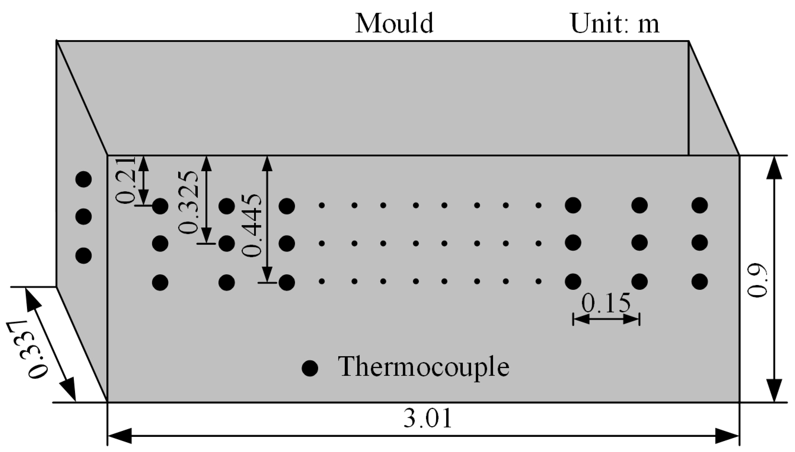
The schematic diagram of the thermocouple arrangement on mold copper plates is shown in Figure 1 [22]. The thermocouples were buried in the copper plates: there were 19 columns of thermocouples on the wide face, with a spacing of 0.15 m, and there was 1 column of thermocouples on the narrow face. Three rows of thermocouples were arranged along the casting direction; these were 0.21, 0.325 and 0.445 m, respectively, below the mold top.
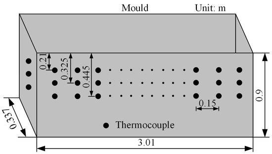
Figure 1.
Schematic diagram of the thermocouple arrangement on mold copper plates.
2.2. Temperature Characteristics of Surface Longitudinal Cracks
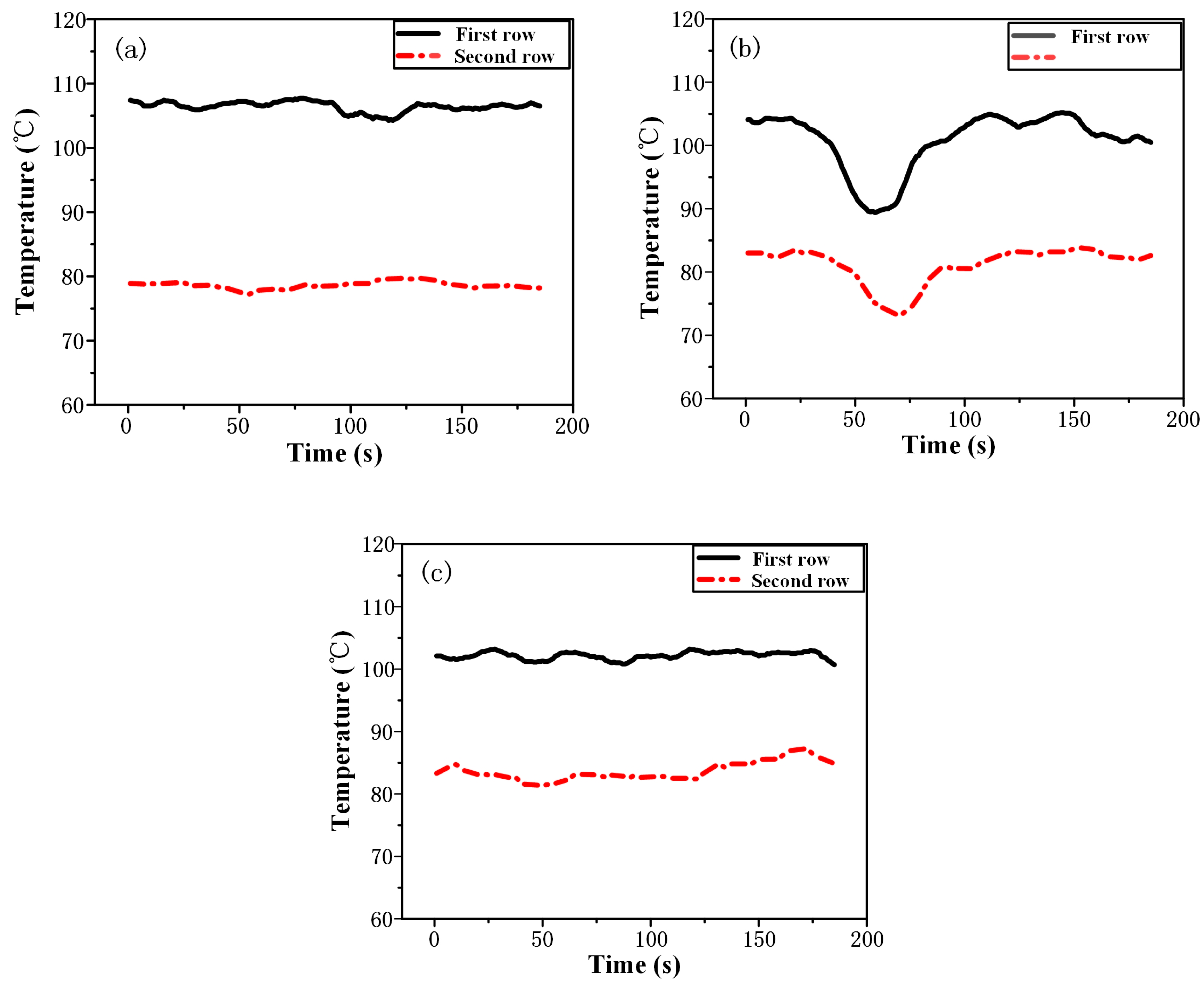
Figure 2 shows the current and adjacent thermocouple temperature curves when a surface longitudinal crack occurred. In this paper, we defined the current and its adjacent thermocouples as the middle, the left and the right thermocouples, respectively. When a longitudinal crack occurred, an air gap appeared with it. This led to a heat-transfer obstruction between the slab and the copper plate. As a result, the temperature of the first row of thermocouples decreased as the longitudinal crack passed through the thermocouples. When the longitudinal crack exited the first row of thermocouples, the heat transfer between the mold and slab returned to normal. Correspondingly, the temperature gradually increased until it returned to normal. The temperature of the middle thermocouples showed a “fall-steady-rise” trend, which also appeared on the second row of thermocouples, as shown in Figure 2b. As the longitudinal crack moved along the casting direction, the left and right thermocouples adjacent to it did not show similar temperature characteristics, as shown in Figure 2a,c.
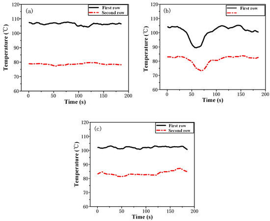
Figure 2.
The current and adjacent thermocouple temperature curves during the occurrence of surface longitudinal cracks. (a) The left thermocouple; (b) the middle thermocouple; (c) the right thermocouple.
2.3. Extraction of Typical Temperature Characteristics of Longitudinal Cracks
According to the “fall-steady-rise” temperature trend, the temperature characteristics were extracted for the middle, left and right thermocouples. As shown in Table 2, a total of 42 dimensional characteristics were extracted, which were used to characterize the characteristics of temperature variation and spatial distribution during the occurrence of longitudinal cracks.
Table 2.
Extraction of longitudinal crack temperature characteristics.
3. Longitudinal Crack Sample Database and Dimension Reduction Using PCA
3.1. Longitudinal Crack Sample Database
A total of 120 samples were selected from a steel plant for the original characteristic database, and included 30 longitudinal crack samples and 90 non-longitudinal crack samples. The non-longitudinal crack samples contained four common conditions, which were large temperature fluctuations, small temperature fluctuations, sticker breakouts and start-up casting, and included the main large temperature fluctuation during the process of continuous casting.
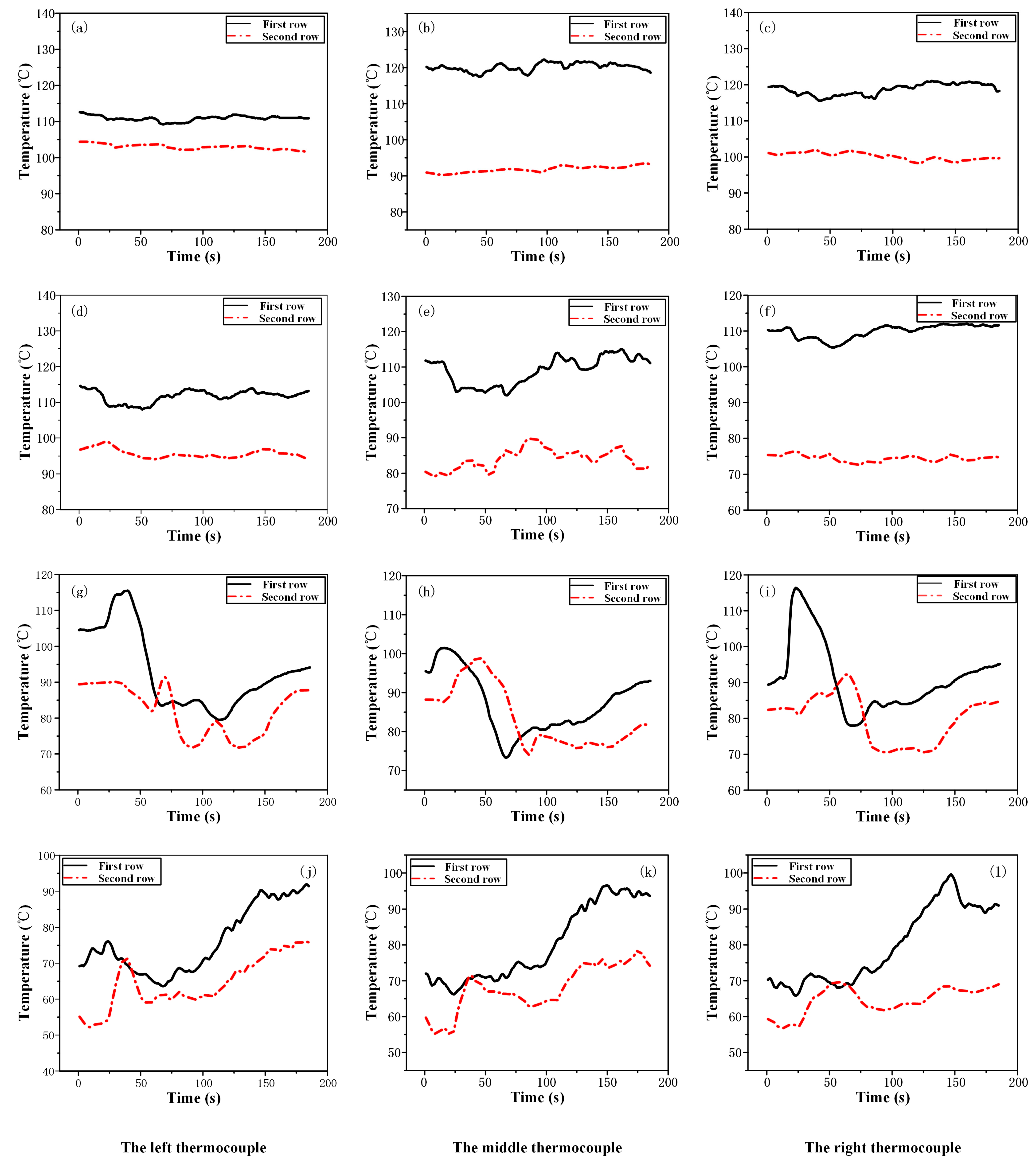
Figure 3 shows the temperature curves of the non-longitudinal crack samples. Figure 3a–c show the temperature curves of the three columns of thermocouples for the small temperature fluctuation samples. The caster was in a stable casting state at this time, the process parameters did not change and the mold was in a stable state. Thus, the fluctuation in the temperature of each thermocouple was small. Figure 3d–f show the temperature curves of the three columns of thermocouples for the large temperature fluctuation samples. It can be seen that the temperature fluctuation was more obvious than for the small temperature fluctuation samples. In the process of continuous casting, the production methods as well as small adjustments to the casting speed, the slag ring and other process operations may lead to this situation. The uneven shrinkage of the local slab shell in the mold during solidification and the uneven distribution of mold powder between the copper plates and the slab can also lead to this situation. Figure 3g–i show the temperature curves of the three columns of thermocouples for the sticker breakout samples. When a breakout occurs, the molten steel inside the slab overflows, which leads to a rapid increase in the thermocouple temperature at the position of sticker. When the sticker passed through the first and second rows of thermocouples in turn, the temperature curve showed an increasing trend. When the sticker exited the first and second rows of thermocouples in turn, the temperature decreased accordingly. Subsequently, due to the operation of increasing the casting speed, the temperature gradually rose to a normal level. This was similar to the temperature changes of the surface longitudinal crack samples. At the same time, because the bonding point laterally propagated to both sides, the same temperature trend appeared in the left and the right thermocouples. Figure 3j–l show the temperature curves of the three columns of thermocouples for the start-up casting samples. At the beginning of casting, the thermocouple temperature continuously rises due to the increase in casting speed. Then, the casting speed gradually stabilizes. The temperature is maintained or slightly decreases. In this process, the system measures the temperature of the steel water. If the temperature is not abnormal after the measurement, the casting speed is increased to a normal level and, correspondingly, the temperature increases to a normal level. At this time, our three columns of thermocouples showed the same trend, as shown in the figures.
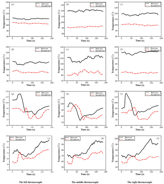
Figure 3.
Temperature curves of non-longitudinal crack samples. (a–c) Small temperature fluctuation samples; (d–f) large temperature fluctuation samples; (g–i) sticker breakout samples; (j–l) start-up casting samples.
3.2. Dimension Reduction of Typical Characteristics Using PCA
A total of 42 dimensional features were obtained from the characteristic extraction, which fully characterized the temperature fluctuations and spatial distribution of longitudinal cracks. However, a correlation and information redundancy between different characteristics may have existed due to the high character dimension. In addition, too many characteristics bring additional computational requirements and interference to the accuracy of the model identification [23]. Therefore, in this paper, the PCA method was used to reduce the dimension of the above characteristics.
The PCA is a commonly used dimension-reduction method. It maps the original n-dimensional feature vector to a new feature space by means of orthogonal transformation and constructs new linearly independent and less numerous k-dimensional vectors. The PCA replaces the overall data features with a smaller number of features, reduces the data dimension and the complexity of the model and then improves the convergence and operational speed of the model.
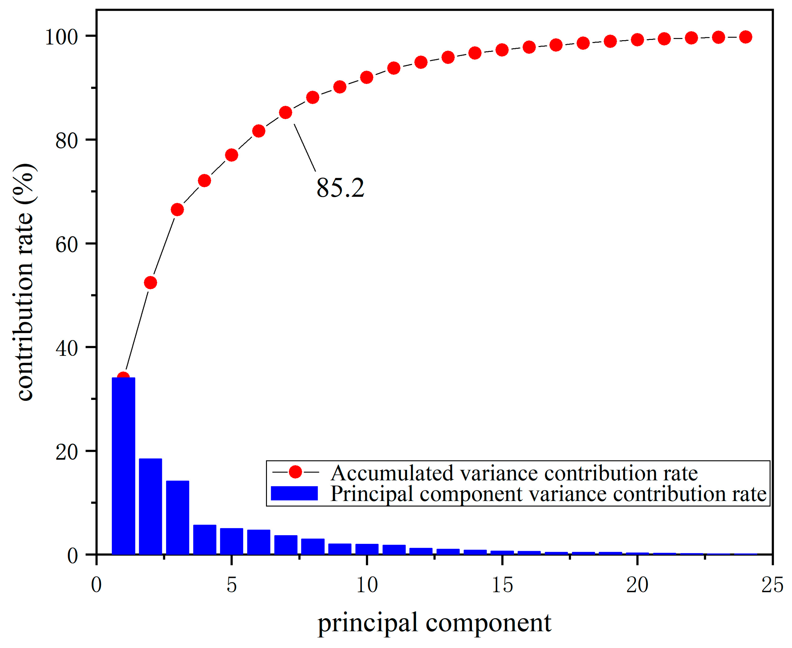
The PCA method uses the cumulative variance contribution rate to characterize how much data from the original information the principal component retains [24]. Figure 4 is the relationship curve between the number of principal components and the variance contribution rate. It can be seen that as the number of principal components increased, more information from the original characteristics was retained. When the number of principal components reached 24, nearly 100% of the original characteristic information was covered.
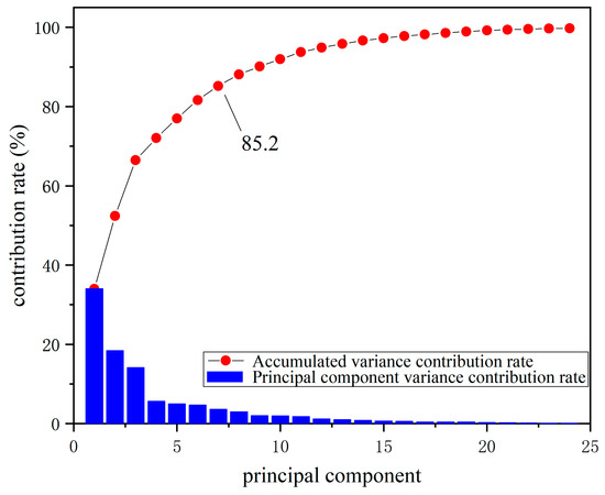
Figure 4.
The relationship between the number of principal components and variance contribution rate.
The variance contribution rate of each principal component was extracted and the results are shown in Table 3. It is generally believed that a principal component analysis can fully characterize the original information when the cumulative contribution rate is higher than 85%. According to Table 3, when the number of principal components was 7, the cumulative variance contribution rate exceeded 85%, which covered the main information of the original data. Therefore, the first 7 principal components were selected to form a new characteristic dataset as the input for the longitudinal crack recognition model.
Table 3.
The variance contribution rate of principal components.
4. Methodology
XGBOOST is a boosting algorithm based on decision trees, which improves the basis of GBDT. XGBOOST adds a regularization term to the objective function on the basis of the GBDT algorithm to reduce the complexity of the model, which improves the generalization ability of the model and effectively prevents overfitting [25]. The Taylor formula is used to expand the loss function in the second order. The first-order and second-order derivatives are used to approximate the objective function to obtain more information to train the tree model, which improves the convergence speed and accuracy of the algorithm [26].
XGBOOST first generates multiple weak classifiers (cart trees), which make joint decisions. Each tree in XGBOOST fits the residual between the previous tree and the real value and iterates until the termination condition is reached. Finally, the fitted results for each tree are weighted and summed to obtain the final prediction of the model. The prediction process of XGBOOST can be summarized as follows.
The model predictions are shown in Equation (1) [27]:
where fk∈F. F is the cart tree space, yi* is the predicted value of the ith sample, xi is the ith sample of the input, fk is the predicted value of the kth tree and K is the number of all subtrees.
The objective function of the model is shown in Equation (2) [28]:
where the first term is the loss function and the second term is the canonical term, the specific form of which is shown in Equation (3) [29]:
where T is the number of leaf nodes in the subtree, ωj is the leaf node weight and γ and λ are coefficients.
The XGBOOST model adopts an addition training mode. If yi*(t) is the predicted value of the ith sample in the tth iteration process, then yi*(t) can be represented by Equation (4) [30]:
Then, the objective function can be rewritten as Equation (5) [31]:
At this time, the Ω(fk) of the first t−1 trees is known, which is a constant, and the objective function can be rewritten as Equation (6) [31]:
where the C is a constant.
The above formula is expanded by the second-order Taylor expansion, as shown in Equation (7) [32]:
where gi is the first-order partial derivative of the loss function and hi is the second-order partial derivative of the loss function, as shown in Equations (8) and (9) [33], respectively:
where yi and yi*(t−1) are known. In the process of solving the minimum value of the objective function, the constant term has no effect on the result. Therefore, the simplified objective function after removing the constant term is as shown in Equation (10) [34]:
The function prediction value ft(xi) is transformed into the corresponding leaf node weight value of the tree and the mapping function q is established. q(xi) represents the position of the leaf node where the current xi sample is located and the weight of this leaf node is ω. Then, we have f(xi) = ω(xi). It is shown in Equation (11) [34]:
where γ is the penalty strength, T is the number of leaf nodes, ω is the leaf weight, q represents the corresponding leaf nodes when the actual sample is mapped to the tree structure and q(xi) represents the number of leaf nodes.
Subsequently grouping the leaf nodes, we classified all samples of xi belonging to the jth leaf node into the same sample set, which is shown in Equation (12) [28]. Gi represents the cumulative sum of the first-order partial derivatives of all samples at leaf node j, as shown in Equation (13) [33]. Hi represents the cumulative sum of the second-order partial derivatives of all samples at leaf node j, as shown in Equation (14) [33]:
At this point, the objective function is further simplified, as shown in Equation (15) [35]:
The objective function is transformed into a unary quadratic function about ωj. The optimal weight value ωj* and the optimal loss function obj* are obtained, as shown in Equations (16) and (17) [35], respectively:
However, there are many parameters in the XGBOOST model that influence the evaluation scores and cannot be manually determined. The PSO algorithm is suitable for the optimization work of a large number of parameters. Moreover, the PSO algorithm is widely used because of its simple structure and high optimization efficiency [36]. Therefore, the PSO method was used to obtain the optimal parameter combination for the XGBOOST model in this paper.
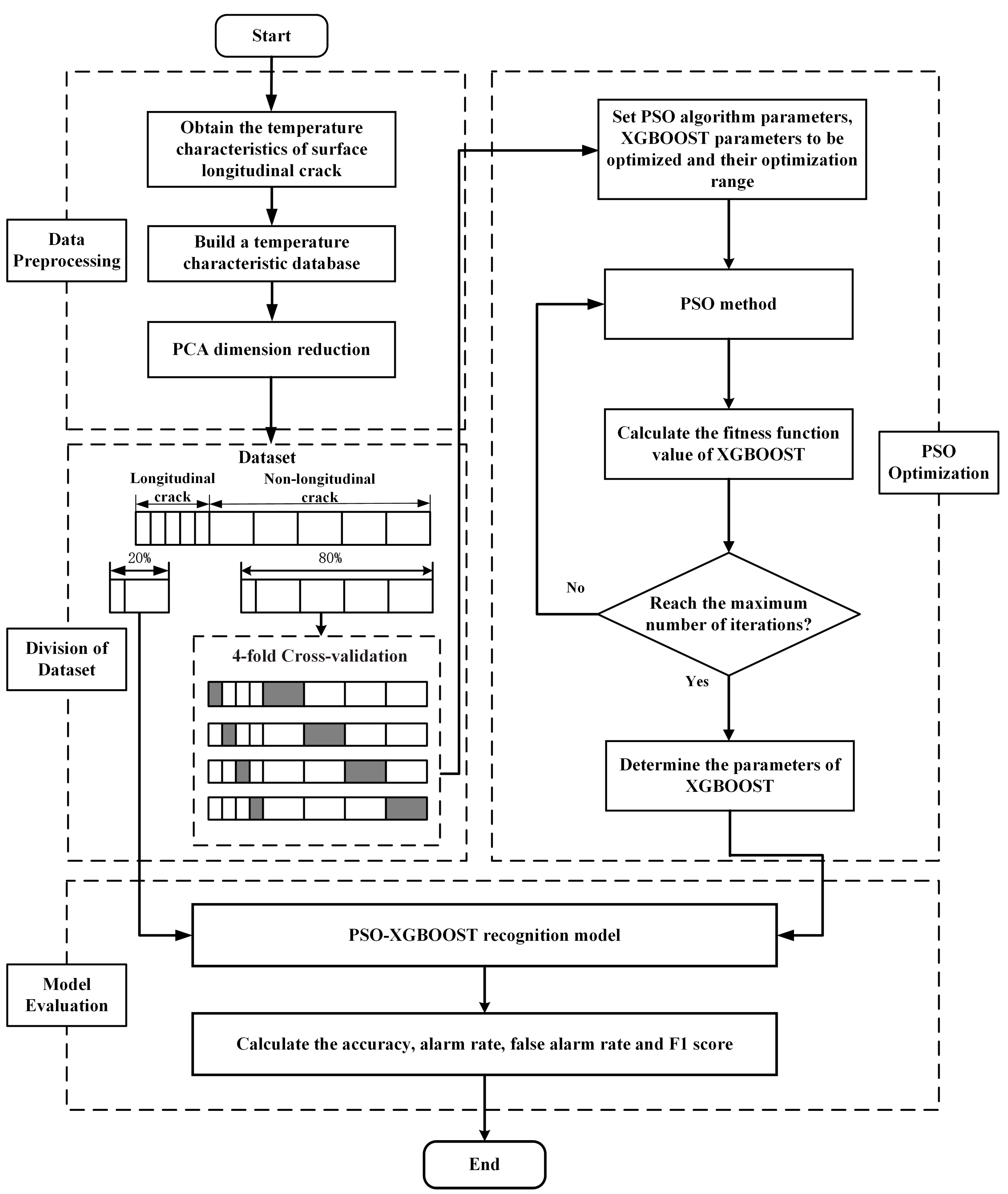
The PSO algorithm originated from research on the predation behavior of bird groups [37]. Firstly, the algorithm designs a massless particle swarm to simulate the foraging of birds. In each iteration, each particle separately searches for the optimal position in the solution space, which is labeled as the current individual optimal position. Secondly, the current individual optimal position is shared with the whole particle swarm and the optimal individual position in the whole particle swarm is obtained as the current global optimal position. Finally, the optimal solution of the model is obtained through multiple iterations. In this study, an identification model based on PSO-XGBOOST was established to identify the surface longitudinal cracks of continuous casting slabs. Firstly, the data were preprocessed. The temperature signal was extracted and analyzed when a surface longitudinal crack occurred and the temperature characteristics were obtained. Based on the actual data of the plant, a temperature characteristic database was built, which contained the samples of longitudinal cracks and non-longitudinal cracks. The PCA method was used to reduce the dimension of the database and the new characteristic database obtained after the dimension reduction was used to test and train the model. Secondly, we divided the dataset. Based on the new characteristic database after the PCA dimension reduction, a stratified sampling method was used to divide the database by 8:2. Among them, 80% of the samples were used as the training set for the optimization training of the XGBOOST model and 20% of the samples were used as the testing set for the performance evaluation of the XGBOOST model. Thirdly, PSO was used to optimize the parameters. We then set the PSO algorithm parameters, the XGBOOST parameters and their optimization range. PSO was used to determine the optimal parameter combination of XGBOOST. Finally, we evaluated the model. Based on the optimal parameter combination, the PSO-XGBOOST surface longitudinal crack identification model was constructed. Based on the confusion matrix, the accuracy, the alarm rate, the false alarm rate and the F1 score were selected as the evaluation metrics of the model. Based on the prediction results of the model, the accuracy, the alarm rate, the false alarm rate and the F1 score of the model were calculated to evaluate the performance of the PSO-XGBOOST recognition model. The overall model building process is shown in Figure 5.

Figure 5.
Flow chart of longitudinal crack recognition model based on PSO-XGBOOST.
5. Results and Discussion
5.1. Evaluation Indexes
The confusion matrix is included in Table 4, and consisted of the actual class and predicted class. TP, FP, FN and TN in the table represent the number of true-positive, false-positive, false-negative and true-negative samples, respectively.
Table 4.
Confusion matrix.
Based on the confusion matrix, the accuracy, the alarm rate, the false alarm rate and the F1 score were selected as the evaluation indexes of the models, which were calculated by Equations (18)–(21):
5.2. The Results of PSO Optimization
For XGBOOST parameter optimization, the population size of PSO, the maximum number of iterations, the inertia weight (w) and the acceleration factors c1 and c2 were 40, 300, 0.729, 1.494 and 1.494, respectively. The maximum accuracy mean of the four-fold cross-validation was used to determine the optimal parameters. The parameters, the optimal range and the optimization results are included in Table 5. The final optimal parameters were as follows: learning_rate = 0.2; n_estimators = 309; max_depth = 4; min_child_weight = 1; gamma = 0.2; reg_lambda = 0.1; subsample = 0.84; colsample_bytree = 0.5.
Table 5.
PSO optimization results.
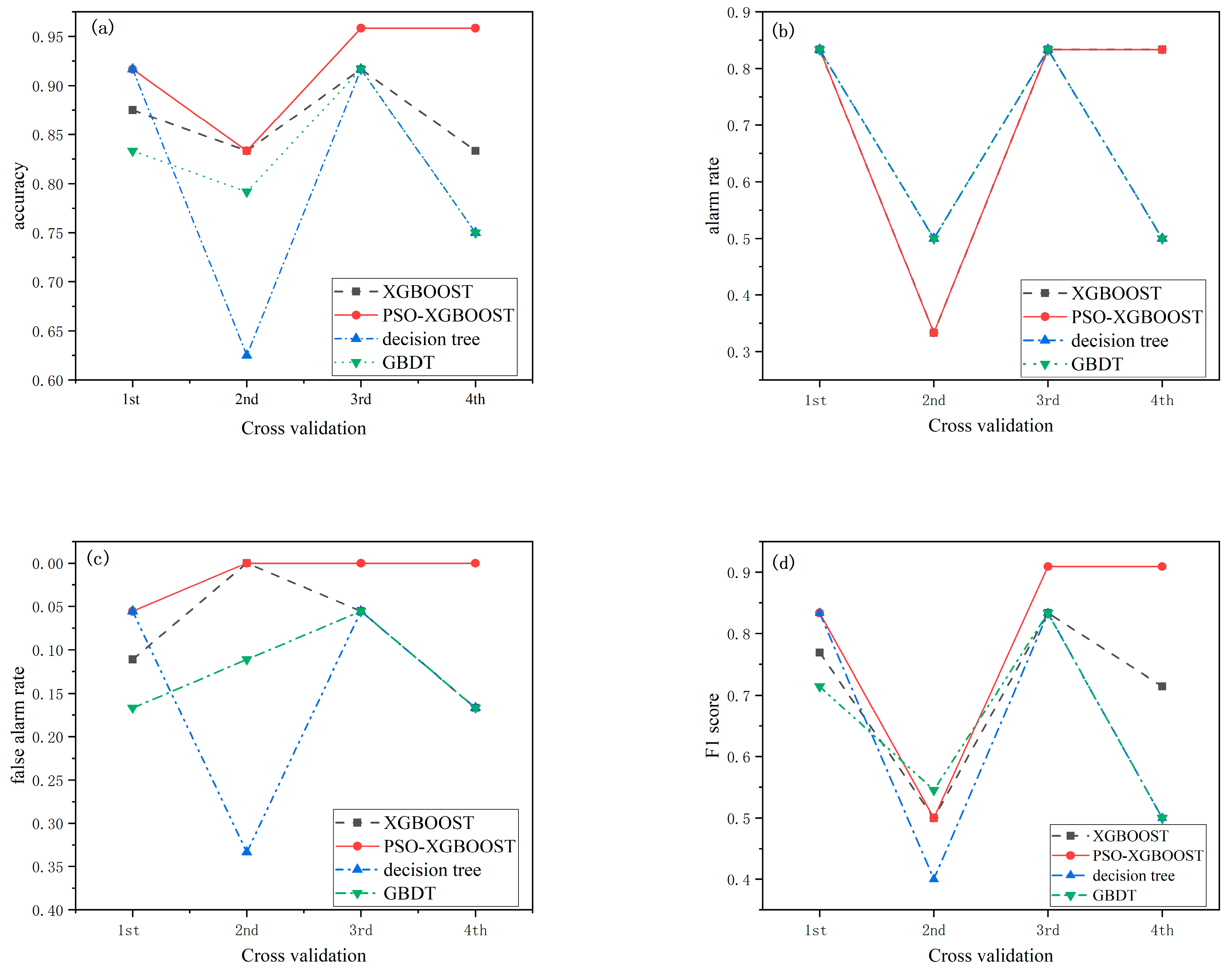
Based on four-fold cross-validation, the PSO-XGBOOST, XGBOOST, decision tree and GBDT models were trained. It can be seen in Figure 6 that PSO-XGBOOST had the best performance followed by XGBOOST, GBDT and the decision tree. The PSO-XGBOOST accuracy reached 95.8%. The highest alarm rate was 83.3%, the F1 score reached 90.9% and the false alarm rates were as low as 0 in the second, third and fourth validations, reflecting the excellent recognition performance. From the four-fold cross-validation, we ascertained that PSO-XGBOOST had the better performance, 3 times greater than XGBOOST in accuracy, the false alarm rate and the F1 score. This indicated that the PSO method could stably improve the performance of the XGBOOST model, increasing its recognition capability.
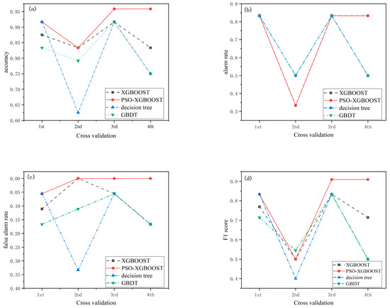
Figure 6.
Cross-validation process: (a) accuracy; (b) alarm rate; (c) false alarm rate; (d) F1 score.
5.3. Discussion of Testing Results
The testing results of the PSO-XGBOOST, XGBOOST, decision tree and GBDT models are included in Table 6. All the longitudinal crack samples could be recognized by PSO-XGBOOST, XGBOOST and the decision tree. However, there were three occurrences of false recognition with decision tree model and two occurrences of false recognition for the XGBOOST model. PSO-XGBOOST had only one occurrence of false recognition, which showed better recognition accuracy. There was one longitudinal crack sample that was not recognized by GBDT and three occurrences of false recognition.
Table 6.
Confusion matrix of test results.
Figure 7 shows the testing evaluation indexes of the four models. It can be seen that PSO-XGBOOST had the best performance in all evaluation indexes, in which the accuracy, F1 score and alarm rate were all above 90% and the false alarm rate was as low as 5.5%. The order of the prediction accuracy of each model was PSO-XGBOOST > XGBOOST > decision tree > GBDT. Among them, PSO-XGBOOST achieved an F1 score of 95.8%, which demonstrated an improvement of 6.6%, 12.3% and 20.9% compared with XGBOOST, decision tree and GBDT, respectively.
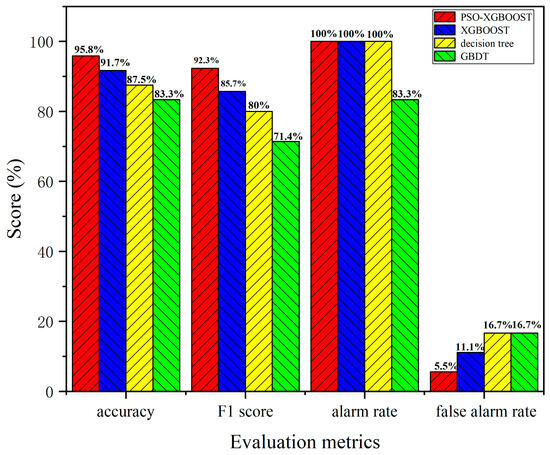
Figure 7.
Evaluation metrics for test sets of four models.
6. Conclusions
- (1)
- In this paper, a sample database was established using all 120 samples from actual casting data of a steel plant, which consisted of longitudinal cracks and non-longitudinal cracks. The non-longitudinal crack samples contained four common conditions, which were large temperature fluctuations, small temperature fluctuations, sticker breakouts and start-up casting, and included the main large temperature fluctuation during the process of continuous casting. The 42 dimensions of the typical temperature characteristics of the middle, left and right thermocouples were extracted. The PCA method was used to reduce the original characteristic dimension from 42 to 7 on the premise of fully retaining the original information, eliminating the redundant information and reducing the complexity of the modeling operations.
- (2)
- The PSO method was used to optimize the XGBOOST model and the optimal model parameters were obtained. PSO-XGBOOST had best identification performance in all evaluation indexes, in which the accuracy reached 95.8%, the highest alarm rate was 83.3%, the F1 score reached 90.9% and the false alarm rates were as low as 0. The results revealed that the particle swarm optimization algorithm could significantly improve the identification performance of XGBOOST. The results also reflected the effectiveness of PSO in multi-parameter optimization.
- (3)
- Based on a four-fold cross-validation, PSO-XGBOOST was compared with XGBOOST, GBDT and decision tree methods on the training set. The order of the prediction accuracy of each model was PSO-XGBOOST > XGBOOST > decision tree > GBDT. Among them, PSO-XGBOOST achieved an F1 score of 95.8%, which was an improvement of 6.6%, 12.3% and 20.9% compared with XGBOOST, decision tree and GBDT, respectively. By comparison with other commonly used models, the superiority of the PSO-XGBOOST model also reflected the effectiveness of the database establishment and feature extraction methods used in this paper. The research results provide a theoretical basis and a reliable model for surface longitudinal crack identification.
Author Contributions
Conceptualization, Y.L.; methodology, L.J.; software, Y.L.; validation, J.L., J.S., Z.Z. and G.L.; formal analysis, Y.L. and J.L.; investigation, Y.L. and J.L.; resources, Y.L., G.L. and J.S.; data curation, Y.L. and L.J.; writing—original draft preparation, Y.L. and L.J.; writing—review and editing, J.L., Z.Z., J.S., G.L. and Z.W.; visualization, J.L. and Z.Z.; supervision, J.S., Z.W. and G.L.; project administration, J.S. and G.L.; funding acquisition, Y.L. All authors have read and agreed to the published version of the manuscript.
Funding
This research was funded by the National Natural Science Foundation of China (51704073/51974056) and the Science and Technology Research Project of Jilin Provincial Education Department (JJKH20230111KJ).
Data Availability Statement
The data that support the findings of this study are available on request from the corresponding author. The data are not publicly available due to privacy or ethical restrictions.
Conflicts of Interest
The authors declare no conflicts of interest.
References
- Swain, A.N.S.S.; Choudhary, S.K. Effect of initial solidification characteristics on longitudinal crack formation in thin slab caster. Can. Metall. Q. 2022, 62, 372–382. [Google Scholar] [CrossRef]
- Roy, S.; Singh, R.K. Investigation of Genesis of Internal Subsurface Crack in Continuous Cast Slabs and Finding Remedial Measures. J. Fail. Anal. Prev. 2023, 23, 2633–2639. [Google Scholar] [CrossRef]
- Zhang, Q.; Yang, J. Characteristics of Inclusions and Microstructures Around Solidification Hook of Low-Carbon Steel Continuous Casting Slab. Metall. Mater. Trans. B 2023, 54, 2439–2453. [Google Scholar] [CrossRef]
- Kamaraj, A.; Haldar, N. High-temperature simulation of continuous casting mould phenomena. Trans. Indian Inst. Met. 2020, 73, 2025–2031. [Google Scholar] [CrossRef]
- Zhu, M.; Cai, Z. Formation Mechanism and Control Technology of Transverse Corner Cracks During Slab Continuous Casting of Microalloyed Steels. Steel Res. Int. 2023, 94, 2300119. [Google Scholar] [CrossRef]
- Peng, Z.; Mei, T. Cracking Behavior and High-Temperature Thermoplastic Analysis of 09CrCuSb Steel Billets. Metals 2023, 13, 1058. [Google Scholar] [CrossRef]
- Thomas, B.G. Review on modeling and simulation of continuous casting. Steel Res. Int. 2018, 89, 1700312. [Google Scholar] [CrossRef]
- Du, F.; Wang, X. Prediction of longitudinal cracks based on a full-scale finite-element model coupled inverse algorithm for a continuously cast slab. Steel Res. Int. 2017, 88, 1700013. [Google Scholar] [CrossRef]
- Fedosov, A.V.; Skrebtsov, A.M. Formation of transverse surface cracks during peritectic steel continuous casting. Metallurgist 2018, 62, 39–48. [Google Scholar] [CrossRef]
- Louhenkilpi, S.; Miettinen, J. New phenomenological quality criteria for continuous casting of steel based on solidification and microstructure tool IDS. Ironmak. Steelmak. 2021, 48, 170–179. [Google Scholar] [CrossRef]
- Klug, J.L.; Medeiros, S.L.S. Designing mould fluxes to prevent longitudinal cracking for peritectic steel slab casting. Ironmak. Steelmak. 2023, 50, 1451–1464. [Google Scholar] [CrossRef]
- Irie, S.; Tsuzumi, K. Estimation of changes in content and characteristics of mold flux during continuous casting. ISIJ Int. 2023, 63, 516–524. [Google Scholar] [CrossRef]
- Zhou, J.; Zhu, L. Analysis of the Formation Mechanism of Surface Cracks of Continuous Casting Slabs Caused by Mold Wear. Processes 2022, 10, 797. [Google Scholar] [CrossRef]
- Presoly, P.; Pierer, R. Identification of defect prone peritectic steel grades by analyzing high-temperature phase transformations. Metall. Mater. Trans. A 2013, 44, 5377–5388. [Google Scholar] [CrossRef]
- Xing, L.; Wang, M. Study on surface longitudinal crack formation of typical hypoeutectoid steel produced on a caster with billet and slab. Metals 2019, 9, 1269. [Google Scholar] [CrossRef]
- Kromhout, J.A.; Schimmel, R.C. Understanding mould powders for high-speed casting. Ironmak. Steelmak. 2018, 45, 249–256. [Google Scholar] [CrossRef]
- Furumai, K.; Zurob, H.S. Influence of mould level instability on the unevenness of solidified shell deformations during continuous casting. Ironmak. Steelmak. 2023, 50, 818–827. [Google Scholar] [CrossRef]
- Velička, M.; Pyszko, R. Research on Solid Shell Growth during Continuous Steel Casting. Materials 2023, 16, 5302. [Google Scholar] [CrossRef]
- Du, F.; Wang, X. Analysis of the non-uniform thermal behavior in slab continuous casting mold based on the inverse finite-element model. J. Mater. Process. Tech. 2014, 214, 2676–2683. [Google Scholar] [CrossRef]
- Landstrom, A.; Thurley, M.J. Morphology-based crack detection for steel slabs. IEEE J. Sel. Top. Signal Process. 2012, 6, 866. [Google Scholar] [CrossRef]
- Duan, H.; Wei, J. Longitudinal Crack Detection Approach Based on Principal Component Analysis and Support Vector Machine for Slab Continuous Casting. Steel Res. Int. 2021, 92, 2100168. [Google Scholar] [CrossRef]
- Liu, Y.; Jiang, L. Mould heat transfer and friction behavior on the surface of wide and heavy slabs in the presence of longitudinal cracks. Metall. Res. Technol. 2023, 120, 314. [Google Scholar] [CrossRef]
- Hasan, B.M.S.; Abdulazeez, A.M. A review of principal component analysis algorithm for dimensionality reduction. J. Soft Comput. Data Min. 2021, 2, 20–30. [Google Scholar]
- Emerson, R.W. A look at principal component analysis. J. Vis. Impair. Blind. 2020, 114, 240–242. [Google Scholar] [CrossRef]
- Sagi, O.; Rokach, L. Approximating XGBoost with an interpretable decision tree. Inform. Sci. 2021, 572, 522–542. [Google Scholar] [CrossRef]
- Ogunleye, A.; Wang, Q.G. XGBoost model for chronic kidney disease diagnosis. IEEE/ACM Trans. Comput. Biol. Bioinform. 2019, 17, 2131–2140. [Google Scholar] [CrossRef] [PubMed]
- Jabeur, S.B.; Mefteh-Wali, S. Forecasting gold price with the XGBoost algorithm and SHAP interaction values. ANN Oper. Res. 2024, 334, 679–699. [Google Scholar] [CrossRef]
- Wang, M.; Li, Y. An XGBoost-SHAP approach to quantifying morphological impact on urban flooding susceptibility. Ecol. Indic. 2023, 156, 111137. [Google Scholar] [CrossRef]
- Tarwidi, D.; Pudjaprasetya, S.R. An optimized XGBoost-based machine learning method for predicting wave run-up on a sloping beach. MethodsX 2023, 10, 102119. [Google Scholar] [CrossRef]
- Qiu, Y.; Zhou, J. Short-term rockburst damage assessment in burst-prone mines: An explainable XGBOOST hybrid model with SCSO algorithm. Rock Mech. Rock Eng. 2023, 56, 8745–8770. [Google Scholar] [CrossRef]
- Li, Y.C. A county-level soybean yield prediction framework coupled with XGBoost and multidimensional feature engineering. Int. J. Appl. Earth Obs. 2023, 118, 103269. [Google Scholar] [CrossRef]
- Punuri, S.B.; Kuanar, S.K. Efficient net-XGBoost: An implementation for facial emotion recognition using transfer learning. Mathematics 2023, 11, 776. [Google Scholar] [CrossRef]
- Jovanovic, L.; Jovanovic, G. The explainable potential of coupling metaheuristics-optimized-xgboost and shap in revealing vocs’ environmental fate. Atmosphere 2023, 14, 109. [Google Scholar] [CrossRef]
- Li, L.; Zhao, Y. An XGBoost Algorithm Based on Molecular Structure and Molecular Specificity Parameters for Predicting Gas Adsorption. Langmuir 2023, 39, 6756–6766. [Google Scholar] [CrossRef]
- Jovanovic, G.; Perisic, M. Potential of coupling metaheuristics-optimized-XGBoost and SHAP in revealing PAHs environmental fate. Toxics 2023, 11, 394. [Google Scholar] [CrossRef]
- Wang, D.; Tan, D. Particle swarm optimization algorithm: An overview. Soft Comput. 2018, 22, 387–408. [Google Scholar] [CrossRef]
- Marini, F.; Walczak, B. Particle swarm optimization (PSO). A tutorial. Chemom. Intell. Lab. Syst. 2015, 149, 153–165. [Google Scholar] [CrossRef]

Disclaimer/Publisher’s Note: The statements, opinions and data contained in all publications are solely those of the individual author(s) and contributor(s) and not of MDPI and/or the editor(s). MDPI and/or the editor(s) disclaim responsibility for any injury to people or property resulting from any ideas, methods, instructions or products referred to in the content. |
© 2024 by the authors. Licensee MDPI, Basel, Switzerland. This article is an open access article distributed under the terms and conditions of the Creative Commons Attribution (CC BY) license (https://creativecommons.org/licenses/by/4.0/).