Approach to Chemical Process Transition Control via Regulatory Controllers with the Case of a Throughput Fluctuating Ethylene Column

Abstract

For chemical processes, dynamic optimization is employed for process transition. On the basis of the multilayer control structure, the employment of dynamic optimization is affected by the regulatory control system. To avoid the adjustment of the regulatory control system, set-point optimization is proposed. For comparison, two types of optimization models, namely direct optimization and set-point optimization, are formulated. The superiority of set-point optimization is rigorously proven. By simulating the commercial process of a throughput-fluctuating ethylene column, the integrated absolute error and maximum deviation of product quality are reduced by more than 150% with set-point optimization. The results indicate that the approach to process transition via regulatory controllers not only avoids the insecurity caused by the switching of set-point controllers but also improves the optimization performance. In conclusion, the proposed optimization structure, namely set-point optimization, is operable and stable for commercial chemical process transitions.

1. Introduction

For continuous chemical processes, the process transition caused by the flexible working conditions should be considered [1,2,3], whereas the requirement for dynamic processes may not be satisfied by the general control system. There is a necessity to improve the process performance with complicated control strategies.

In the previous work of the authors [2], control vector parameterization (CVP) was used for implementing the process transition. The decision variables of the optimization problem contain the discrete time grid and the parametric sequence, and the performance is improved by the alternation optimization. Through the simulation of the practical chemical process, innovation and practicability have been verified.

Despite employing dynamic optimization structures to improve dynamic performance [4], there is a major problem for practical application. In commercial chemical processes, because of their complexity and reconfigurability [5], the multilayer control structure is widely used [6]. Only the basic control layer has direct access to the plant [7]. In other words, the outputs of the dynamic optimization module cannot directly manipulate the plant [8]. Therefore, the regulatory/basic controllers should be considered for the process transition based on dynamic optimization.

Dynamic optimization is recommended for guiding the process transition, whereas the research on dynamic optimization covers a wide range, such as dynamic prediction [9], robust control [10], and nonlinear optimization [11]. Because of their complexity and practicability, the solution strategies of dynamic optimization catch researchers’ attention [12]. Besides the inefficient analytical/variational approach, the numerical approach is recommended for complicated chemical processes [13]. The numerical approach is separated into two groups: simultaneous strategies and sequential strategies [14]. Simultaneous strategies, namely full discretization strategies [15], discretize all the state and control variables, which consume a lot of computational expense for solving the NLP problem. Sequential strategies, namely partial discretization strategies [16,17], just discretize control variables, whereas numerical integration of the DAE model is required [18]. The two approaches are recommended for different commercial plants.

Considering the practical application of dynamic optimization, the set-point optimization structure is employed [19,20]. The decision variables are the set-points of regulatory controllers. In general, there are two important problems caused by regulatory controllers for dynamic optimization. The first problem is establishing a new relevant dynamic model [21,22]. The original process dynamic model is unusable because the decision variables, namely the input of the plant, are changed [23,24]. The second problem is eliminating the influence of regulatory controllers’ performance on dynamic optimization [25]. The poor performance of regulatory controllers leads to the belated tracking of the optimal set-point trajectory [26,27]. Therefore, parameter tuning is necessary for regulatory controllers [28].

To solve the two problems, the scholars proposed the integration of control and process design [29,30]. The dynamic optimal trajectory, regulatory control structures, and controller parameters are obtained by solving a mixed-integer dynamic optimization problem [31,32]. The regulatory control system is adjusted for optimization. But generally, the process transition is occasional for the total process. That is to say, the process transition strategy, such as dynamic optimization, is an auxiliary of the regulatory control strategy. Only when the requirement of dynamic processes cannot be satisfied by the general control system is the process transition strategy adopted. In a word, the regulatory control system is the precondition for implementing the process transition strategy, whereas the adjustment of the regulatory control structures should be avoided for most chemical processes.

This paper is the continuation of the authors’ previous work [2]. The previous work implemented the process transition based on dynamic optimization and proposed an efficient solution strategy based on control vector parameterization. In this paper, the approach to chemical process transition via regulatory controllers is discussed for practical application. For innovation, two types of dynamic optimization models, namely direct optimization and set-point optimization, are proposed and formulated based on the regulatory control structure. The merit of set-point optimization is theoretically proven. For practicality, the fluctuation caused by the adjustment of regulatory control structure is avoided, and the correctness of the theoretical analysis is verified via the case study of a commercial ethylene column with fluctuating throughput.

The detailed contributions are as follows: In Section 2, considering the influence of regulatory controllers, two types of optimization models, namely direct optimization and set-point optimization, are proposed, whereas the latter optimization model is beneficial to safe operation. In Section 3, the different optimization models are formulated. Furthermore, the superiority of set-point optimization is rigorously proven. In Section 4, a commercial ethylene column is introduced. The process transition, caused by the throughput fluctuation, is implemented by set-point optimization. In Section 5, by simulation, the control performance is significantly improved for set-point optimization. That is to say, safety and optimality are simultaneously achieved by dynamic optimization via regulatory controllers.

2. Problem Description

The previous work of the authors proposes the conception of process transition, and then an efficient solving strategy is discussed for complicated chemical processes [2]. Despite the solution strategy, other factors associated with practical application, have not been discussed. In this paper, an approach to chemical process transition via regulatory controllers is implemented.

For chemical processes, the classical multilayer control structure is shown in Figure 1. The direct control layer is responsible for the safe operation of the process. Because of the rapidity of direct control, the extended process, namely the integration of the direct controllers and the process, is modeled by ignoring the adjusting time of direct controllers [33]. The set-point controllers are located at a higher layer, whose input is the result of steady-state optimization. For process transitions caused by large-range changes in production conditions, the optimal working condition is obtained by steady-state optimization [34]. The target of the set-point control layer is reaching the optimal operating point under new production conditions, whereas the optimality of the dynamic transition process is ignored. To improve the dynamic performance, model-based dynamic optimization is employed [2]. The optimal trajectory is the input of the regulatory control system, which consists of direct controllers and set-point controllers.

There is a noteworthy problem with employing dynamic optimization. In detail, two types of dynamic optimization models, namely direct optimization and set-point optimization, are defined. For direct optimization, the optimized object is the extended process, which is the integration of direct controllers and the process. To avoid the conflict of control signals, the set-point controllers should be cut down for the process transition period and re-enabled for the relatively steady period. The switching of set-point controllers is harmful to safe operation. For set-point optimization, the optimized object is the integration of set-point controllers and the extended process. The regulatory controllers are completely retained, which is beneficial for safe and simple operation. On the other hand, besides the influence on safe operation, optimal performance should be considered for the two types of dynamic optimization. In this paper, the merit of the set-point optimization, which completely retained regulatory controllers, is discussed.

3. Process Transition Strategy via Regulatory Controllers

3.1. Optimization Formulation

For direct optimization, shown in Figure 2a, I_x represents the production index, such as product quality; x_sp represents the set-point; u represents the manipulated variables; and v represents the operating variables. The mode A represents the dynamic optimization enable, and the mode B represents the set-point control enable. Direct control is the basic layer of the control system. Considering reliability and robustness, the optimized object is the extended process, namely the integration of direct controllers and chemical processes, whereas the optimization/decision variables (u) are the inputs of direct controllers.

For set-point optimization, shown in Figure 2b, the optimized object is the integration of set-point controllers and an extended process, whereas the optimization/decision variables (x_sp) are the inputs of set-point controllers. The standard optimization formulation is given in the following description.

To avoid significant superposition error, the full discretization strategy requires high discrete precision, which consumes a lot of computational expense for solving the NLP problem for complicated chemical processes. Considering the large number of state variables, the sequential discretization strategy is recommended to avoid dimension problems. The previous work of the authors proposes the general optimization model [2], which is employed to establish direct and set-point optimization models in the following content.

In Figure 2, to discuss dynamic optimization, there are three parts of the system that should be considered: the set-point control module, the direct control module, and the actual process. The mathematical descriptions of them are represented as:

$$\left\{\begin{array}{c}{f}_{\mathrm{p}}^{\mathrm{d}}(x_{\mathbf{d}},x_{\mathbf{a}},\mathit{v},t)={\dot{x}}_{\mathbf{d}}\\ f_{\mathrm{p}}^{\mathrm{a}}(x_{\mathbf{d}},x_{\mathbf{a}},\mathit{v},t)=0\end{array}\right.$$

(1)

$$f_{\mathrm{dc}}(x_{\mathbf{d}},x_{\mathbf{a}},\mathit{u},t)=\mathit{v}$$

(2)

$$f_{\mathrm{sc}}(x_{\mathbf{d}},x_{\mathbf{a}},{\mathit{x}}_{\mathbf{s}\mathbf{p}},t)=u$$

(3)

where $f_{\mathrm{p}}^{\mathrm{d}}$ and $f_{\mathrm{p}}^{\mathrm{a}}$ represent the differential and algebraic equations of the actual process; $x_{\mathbf{d}}$ and $x_{\mathbf{a}}$ represent the differential and algebraic variables; $\mathit{v}$ represents the input vector of the actual process; $f_{\mathrm{dc}}(\cdot )$ represents the mathematical model of the direct control module; $\mathit{u}$ represents the input vector of the direct control module; $f_{\mathrm{sc}}(\cdot )$ represents the mathematical model of the set-point control module; ${\mathit{x}}_{\mathbf{s}\mathbf{p}}$ represents the input vector of the set-point control module. Meanwhile, the following constraint equations for the inputs should be satisfied:

$$\left\{\begin{array}{c}{\mathit{v}}^{\mathbf{l}\mathbf{b}}\le \mathit{v}(t)\le {\mathit{v}}^{ub}\\ u^{lb}\le \mathit{u}(t)\le u^{ub}\\ {\mathit{x}}_{\mathbf{s}\mathbf{p}}^{\mathbf{l}\mathbf{b}}\le {\mathit{x}}_{\mathbf{s}\mathbf{p}}(t)\le {\mathit{x}}_{\mathbf{s}\mathbf{p}}^{\mathbf{u}\mathbf{b}}\end{array}\right.$$

(4)

where ${\mathit{v}}^{lb}$ and ${\mathit{v}}^{ub}$ are the lower and upper bounds of the input vector for the actual process; ${\mathit{u}}^{lb}$ and $u^{ub}$ are the lower and upper bounds of the input vector for the direct control module; ${\mathit{x}}_{\mathbf{s}\mathbf{p}}^{\mathbf{l}\mathbf{b}}$ and ${\mathit{x}}_{\mathbf{s}\mathbf{p}}^{\mathbf{u}\mathbf{b}}$ are the lower and upper bounds of the input vector for the set-point control module.

For discretization, the control period has been segmented:

$$[0, t_f] \to \begin{array}{cccccc}[0, t_1),& [t_1, t_2),& \cdots ,& [t_{k-1}, t_k),& \cdots ,& [t_{N-1}, t_N]\end{array}$$

(5)

where $t_f$ is the length of control horizon; $t_{k-1}$ and $t_k$ represents the lower and upper time of the k^th time interval; and N is the time interval number.

For direct optimization, the optimized object is an extended process, represented as:

$$\left\{\begin{array}{c}{f}_{\mathrm{ep}}^{\mathrm{d}}(x_{\mathbf{d}},x_{\mathbf{a}},\mathit{u},t)={\dot{x}}_{\mathbf{d}}\\ f_{\mathrm{ep}}^{\mathrm{a}}(x_{\mathbf{d}},x_{\mathbf{a}},\mathit{u},t)=0\end{array}\right.$$

(6)

where $f_{\mathrm{ep}}(\cdot )$ represents the mathematical model of the extended process, namely the integration of Equations (1) and (2). While the direct controllers are idealized, the extended process model is established by process mathematical analysis [33]. The solution is represented as:

$$x=\left[x_{\mathbf{d}},x_{\mathbf{a}}\right]=F_{\mathrm{DC}}(u,t)$$

(7)

where $F_{\mathrm{DC}}(\cdot )$ is obtained by the numerical integration of Equation (6). The optimization vector, namely the input of the direct control module, is represented as:

$$u(t)={\left[\begin{array}{cccccc}{u}^1(t),& u^2(t),& \cdots ,& u^l(t),& \cdots ,& u^{N_{\mathrm{d}}}\left(t\right)\end{array}\right]}^{\mathrm{T}}$$

(8)

where $N_{\mathrm{d}}$ represents the dimension of direct control inputs, discretized/parameterized as:

$$u^l(t)={\displaystyle \sum _{k=1}^{N_{\mathrm{d}}}{\widehat{u}}^{l,k}{\chi }_k(t)}$$

(9)

where ${\widehat{u}}^{l,k}$ represents the value of the l^th optimization variable in $[t_{k-1}, t_k)$. ${\chi }_k(t)$ is represented as:

$${\chi }_k(t)=\left\{\begin{array}{cc}1& \mathrm{if} t_{k-1}\le t<t_k,\\ 0& \mathrm{else}\end{array}\right.$$

(10)

In

Table 1. Formulation of direct optimization and set-point optimization.

	Model 1: Direct Optimization	Model 2: Set-Point Optimization
Optimization objective	$J=\Phi (x,\widehat{u},\chi ,t,t_f)$	$J=\Phi (x,u,\chi ,t,t_f)$
Subject to (s.t.)	$x=F_{\mathrm{DC}}(\widehat{u},\chi ,t)$, $x={[x_{\mathbf{d}},x_{\mathbf{a}}]}^{\mathrm{T}}$, $x_{\mathbf{d}}^{\mathbf{l}\mathbf{b}}\le x_{\mathbf{d}}\le x_{\mathbf{d}}^{\mathbf{u}\mathbf{b}}$, $x_{\mathbf{a}}^{\mathbf{l}\mathbf{b}}\le x_{\mathrm{a}}\le x_{\mathbf{a}}^{\mathbf{u}\mathbf{b}}$, $u^{lb}\le \widehat{u}\le u^{ub}$, $0\le t\le t_f$, ${\displaystyle \sum \chi }=1$	$x=F_{\mathrm{DC}}(u,t)$, $f_{\mathrm{sc}}(x_{\mathbf{d}},x_{\mathbf{a}},{\widehat{\mathit{x}}}_{\mathbf{s}\mathbf{p}},\chi ,t)=u$ $x={[x_{\mathbf{d}},x_{\mathbf{a}}]}^{\mathrm{T}}$, $x_{\mathbf{d}}^{\mathbf{l}\mathbf{b}}\le x_{\mathbf{d}}\le x_{\mathbf{d}}^{\mathbf{u}\mathbf{b}}$, $x_{\mathbf{a}}^{\mathbf{l}\mathbf{b}}\le x_{\mathrm{a}}\le x_{\mathbf{a}}^{\mathbf{u}\mathbf{b}}$, $u^{lb}\le u\le u^{ub}$ ${\mathit{x}}_{\mathbf{s}\mathbf{p}}^{\mathbf{l}\mathbf{b}}\le {\widehat{\mathit{x}}}_{\mathbf{s}\mathbf{p}}\le {\mathit{x}}_{\mathbf{s}\mathbf{p}}^{\mathbf{u}\mathbf{b}}$, $0\le t\le t_f$, ${\displaystyle \sum \chi }=1$
Decision variables	$\chi =[\begin{array}{cccccc}{\chi }_1& {\chi }_2& \cdots & {\chi }_k& \cdots & {\chi }_{N_{\mathrm{dc}}}\end{array}]$$\widehat{u}=\left[\begin{array}{ccccc}{\widehat{u}}^{1,1}& \cdots & {\widehat{u}}^{1,k}& \cdots & {\widehat{u}}^{1,N}\\ ⋮& \ddots & ⋮& \ddots & ⋮\\ {\widehat{u}}^{l,1}& \cdots & {\widehat{u}}^{l,k}& \cdots & {\widehat{u}}^{l,N}\\ ⋮& \ddots & ⋮& \ddots & ⋮\\ {\widehat{u}}^{N_{\mathrm{d}},1}& \cdots & {\widehat{u}}^{N_{\mathrm{d}},k}& \cdots & {\widehat{u}}^{N_{\mathrm{d}},N}\end{array}\right]$	$\chi =[\begin{array}{cccccc}{\chi }_1& {\chi }_2& \cdots & {\chi }_k& \cdots & {\chi }_{N_{\mathrm{sc}}}\end{array}]$${\widehat{\mathit{x}}}_{\mathbf{s}\mathbf{p}}=\left[\begin{array}{ccccc}{\widehat{x}}_{\mathrm{sp}}^{1,1}& \cdots & {\widehat{x}}_{\mathrm{sp}}^{1,k}& \cdots & {\widehat{x}}_{\mathrm{sp}}^{1,N}\\ ⋮& \ddots & ⋮& \ddots & ⋮\\ {\widehat{x}}_{\mathrm{sp}}^{l,1}& \cdots & {\widehat{x}}_{\mathrm{sp}}^{l,k}& \cdots & {\widehat{x}}_{\mathrm{sp}}^{l,N}\\ ⋮& \ddots & ⋮& \ddots & ⋮\\ {\widehat{x}}_{\mathrm{sp}}^{N_{\mathrm{s}},1}& \cdots & {\widehat{x}}_{\mathrm{sp}}^{N_{\mathrm{s}},k}& \cdots & {\widehat{x}}_{\mathrm{sp}}^{N_{\mathrm{s}},N}\end{array}\right]$

, the Model 1 is the mathematical formulation of direct optimization.

The direct optimization model is represented as Model 1 in Table 1.

For set-point optimization, the optimized object is the integration of set-point controllers and an extended process, shown as Equations (3) and (6). The optimization vector, namely the input of the set-point control module, is represented as:

$${\mathit{x}}_{\mathbf{s}\mathbf{p}}(\mathit{t})={\left[x_{\mathrm{sp}}^1\begin{array}{cccccc}(t),& x_{\mathrm{sp}}^2(t),& \cdots ,& x_{\mathrm{sp}}^l(t),& \cdots ,& x_{\mathrm{sp}}^{N_{\mathrm{s}}}\left(t\right)\end{array}\right]}^{\mathrm{T}}$$

(11)

where $N_{\mathrm{s}}$ represents the dimension of set-point control inputs, discretized as:

$$x_{\mathrm{sp}}^l(t)={\displaystyle \sum _{k=1}^{N_{\mathrm{s}}}{\widehat{x}}_{\mathrm{sp}}^{l,k}{\chi }_k(t)}$$

(12)

where ${\widehat{x}}_{\mathrm{sp}}^{l,k}$ represents the value of the l^th optimization variable in $[t_{k-1}, t_k)$. ${\chi }_k(t)$ is represented as Equation (10). Model 2 is the mathematical formulation of set-point optimization.

Direct optimization and set-point optimization are formulated. The difference between them is the involvement of regulatory controllers in dynamic optimization, and the influence of regulatory controllers on optimization performance is discussed in the following section.

3.2. Optimality Comparison

To discuss the difference between direct optimization and set-point optimization, the structural analysis is provided in Figure 3. For direct optimization (Structure-1 in Figure 3a), the optimal result, namely the discrete sequence, directly acts on the extended process. The control performance depends on the deviation caused by the discretization of the optimization vector. For set-point optimization (Structure-2 in Figure 3b), the discrete sequence acts on the integration of set-point controllers and an extended process. By equivalent structure variation, the set-point controller is transformed into a filter, named the equivalent filter (shown in Figure 3d). For instance, while the transfer function of an extended process is simplified as a second-order process, the order of the filter is three. That is to say, the major function of set-point controllers is not constant set-point management, and the softened discrete sequence acts on an extended process. The influence of discrete precision on optimization performance is reduced by the involvement of set-point controllers.

Besides qualitative analysis, rigorous proof is provided for the merits of set-point optimization in the following content. Although the advanced control algorithm catches researcher’s attention, PID control is the conventional strategy. The typical proportional-integral (PI) control algorithm is formulated as:

$$u(t)=K_{\mathrm{p}}\left(e(t)+\frac{1}{T_{\mathrm{i}}}{\displaystyle {\int }_0^{t}e(t)\mathrm{d}t}\right)$$

(13)

where $K_{\mathrm{p}}$ is the proportion parameter; $T_{\mathrm{i}}$ is the integration parameter; $e(t)$ is the error. For set-point optimization, the equation of l^th set-point controller is formulated as:

$$\mathit{u}(\mathit{t})={\mathit{K}}_{\mathbf{p}}\left(\left({\mathit{x}}_{\mathbf{s}\mathbf{p}}(\mathit{t})-{\mathit{x}}_{\mathbf{c}}(\mathit{t})\right)+\frac{1}{{\mathit{T}}_{\mathbf{i}}}{\displaystyle {\int }_0^t\left({\mathit{x}}_{\mathbf{s}\mathbf{p}}(\mathit{t})-{\mathit{x}}_{\mathbf{c}}(\mathit{t})\right)\mathrm{d}t}\right)$$

(14)

where ${\mathit{x}}_{\mathbf{c}}$ is the vector of controlled variables, which satisfies:

$${\mathit{x}}_{\mathbf{c}}(\mathit{t})=\mathbf{M}\mathit{x}(\mathit{t})=\mathbf{M}{F}_{\mathrm{DC}}(\mathit{u}(t),\mathit{t})$$

(15)

where $\mathbf{M}$ represents the output matrix, whose dimension is $N_{\mathrm{s}}\times N_{\mathrm{p}}$. $N_{\mathrm{s}}$ is the number of set-point controllers, whereas $N_{\mathrm{p}}$ is the number of process variables. The Equation (14) is transformed as:

$$\mathit{u}(\mathit{t})={\mathit{K}}_{\mathbf{p}}\left(\left({\mathit{x}}_{\mathbf{s}\mathbf{p}}(\mathit{t})-\mathbf{M}{F}_{\mathrm{DC}}(\mathit{u}(\mathit{t}),\mathit{t})\right)+\frac{1}{{\mathit{T}}_{\mathbf{i}}}{\displaystyle {\int }_0^t\left({\mathit{x}}_{\mathbf{s}\mathbf{p}}(\mathit{t})-\mathbf{M}{F}_{\mathrm{DC}}(\mathit{u}(\mathit{t}),t)\right)\mathrm{d}t}\right)$$

(16)

Equation (16) represents the relationship between ${\mathit{x}}_{\mathbf{s}\mathbf{p}}$ and $\mathit{u}$, namely the function of equivalent filter in Figure 3d. It is obvious that the filter function is determined by the transfer function of extended process. The function is simplified by discretization in the following discussion.

Based on Equation (5), the control horizon is discretized. In the k^th time interval, the controlled variables and manipulated variables are defined as:

$$\left\{\begin{array}{c}{\mathit{x}}_{\mathbf{c}}(\mathit{t})={\mathit{x}}_{\mathbf{c}}^{\mathbf{k}}(\mathit{t}),\\ \mathit{u}(\mathit{t})={\mathit{u}}^{\mathbf{k}}(\mathit{t}),\end{array}\right.\begin{array}{cc} & t\in [t_{k-1}, t_k)\end{array}.$$

(17)

Based on the Fourier series, the l^th controlled variable is formulated as:

$$x_{\mathrm{c}}^{l,k}(t)=x_{\mathrm{c}}^{l,k-1}(t_{k-1})+{\displaystyle \sum _{j=1}^n{a}_j\sin \left(\frac{2\pi j(t-t_{k-1})}{t_f}\right)},\begin{array}{cc} & t\in [t_{k-1}, t_k).\end{array}$$

(18)

where $a$ is the amplitude of the primary function. While the time interval is small enough, Equation (18) is equivalent to Equation (20) based on Equation (19).

$$\underset{t\to \epsilon }{\lim }\left(a_j\frac{2\pi jt}{t_f}-b\left(1-e^{-\frac{t}{T}}\right)\right)=0,\begin{array}{cc} & b\in \mathbf{R}.\end{array}$$

(19)

$$x_{\mathrm{c}}^{l,k}(t)=x_{\mathrm{c}}^{l,k-1}(t_{k-1})+\left(u^{l,k}(t)-u^{l,k-1}(t_{k-1})\right)\left(1-e^{-\frac{(t-t_{k-1})}{T}}\right),\begin{array}{cc} & t\in [t_{k-1},\begin{array}{c} \end{array}{t}_k).\end{array}$$

(20)

Based on Equations (15), (16), and (20), the control equation of lth set-point controller in kth time interval is represented as:

$$\Delta u^{l,k}(t)=K_{\mathrm{p}}^{l,k}\left({\widehat{x}}_{\mathrm{sp}}^{l,k}-x_{\mathrm{c}}^{l,k-1}(t_{k-1})-\Delta u^{l,k}(t)\left(1-e^{-\frac{(t-t_{k-1})}{T}}\right)\right)+\frac{K_{\mathrm{p}}^{l,k}}{T_{\mathrm{i}}^{l,k}}{\displaystyle {\int }_{t_{k-1}}^{t_k}\left({\widehat{x}}_{\mathrm{sp}}^{l,k}-x_{\mathrm{c}}^{l,k-1}(t_{k-1})-\Delta u^{l,k}(t)\left(1-e^{-\frac{(t-t_{k-1})}{T}}\right)\right)dt}$$

(21)

where $\Delta u^{l,k}(t)$ satisfies:

$$\Delta u^{l,k}(t)=u^{l,k}(t)-u^{l,k-1}(t_{k-1}),\begin{array}{cc} & t\in [t_{k-1}, t_k).\end{array}$$

(22)

$t_{k-1}$ is the initial moment, and defining $\overline{t}=t-t_{k-1}$, Equation (22) is transformed as:

$$\Delta u^{l,k}(\overline{t})=u^{l,k}(\overline{t})-u^{l,k-1}(0),\begin{array}{cc} & \overline{t}\in [0, t_k-t_{k-1}).\end{array}$$

(23)

And then, Equation (21) is transformed as:

$$\Delta u^{l,k}(\overline{t})=K_{\mathrm{p}}^{l,k}\left({\widehat{x}}_{\mathrm{sp}}^{l,k}-x_{\mathrm{c}}^{l,k-1}(0)-\Delta u^{l,k}(\overline{t})\left(1-e^{-\frac{\overline{t}}{T}}\right)\right)+\frac{K_{\mathrm{p}}^{l,k}}{T_{\mathrm{i}}^{l,k}}{\displaystyle {\int }_0^{\overline{t}}\left({\widehat{x}}_{\mathrm{sp}}^{l,k}-x_{\mathrm{c}}^{l,k-1}(0)-\Delta u^{l,k}(\overline{t})\left(1-e^{-\frac{\overline{t}}{T}}\right)\right)d\overline{t}}$$

(24)

There is a particular solution of Equation (24), shown as:

$$\left\{\begin{array}{l}{K}_{\mathrm{p}}^{l,k}=1\\ T_{\mathrm{i}}^{l,k}=T\\ u^{l,k}(\overline{t})={\widehat{x}}_{\mathrm{sp}}^{l,k}-x_{\mathrm{c}}^{l,k-1}(0)+u^{l,k-1}(0)\end{array}\right.$$

(25)

where $u^{l,k}(\overline{t})$ is fixed in $\overline{t}\in [0, t_k-t_{k-1})$.

From the above, while the time interval is small enough, the outputs of set-point controllers are constant. The set-point optimization is equivalent to the direct optimization. In other words, the performance of set-point optimization is not lower than the performance of direct optimization.

In the following section, the change of working condition for a throughput-fluctuation ethylene column is implemented by dynamic optimization. And then, the superiority of set-point optimization, which completely retains regulatory controllers, is verified.

4. Throughput-Fluctuating Ethylene Column

The experiment unit of this paper is commercial ethylene equipment. The process transition should be discussed while the decoking of cracking furnaces leads to a fluctuation in throughput. The diagram of the system, which consists of two parts: process (ethylene column) and regulatory controllers (direct and set-point controllers), is shown in Figure 4.

The direct control layer consists of a cold flow controller, a side draw flow controller, and a heat flow controller, whereas the optimization variables are selected from the set-values of the three flow controllers for direct optimization. The set-point control layer consists of the top pressure controller, reflux ratio controller, and bottom temperature controller, whereas the optimization variables are selected from the set-value of the three property controllers for set-point optimization.

Because the adjusting time of direct controllers is much shorter than the response time of an ethylene column, direct controllers are idealized. The mathematical model of the extended process, which consists of an ethylene column and three flow controllers, was established in the authors’ previous work [33]. Due to the limited length and innovative discussion of this paper, the detailed mathematical model, namely the differential and algebraic equations, is not displayed. In brief, the mathematical model is represented as Equation (6), whereas the number of differential variables and equations is 1350, the number of algebraic variables is 2426, the number of algebraic equations is 1818, and the number of independent/manipulated variables is 608. Most of the manipulated variables are assigned by commercial conditions. In this paper, the discussed manipulated variables contain the cold flow rate of the condenser, the heat flow rate of the reboiler, and the molar flow rate of the ethylene product.

In addition, based on the practical situation, the control algorithm is PI for the three set-point controllers. The target of set-point control is satisfying the product quality requirement under the premise of production safety. The main product for the ethylene column is the ethylene product, and the main factor affecting safety is the pressure fluctuation. The fluctuation of ethylene quality is the major challenge, whereas the operating pressure is rapidly stabilized by manipulating the cold flow rate of the condenser. Therefore, the optimization objective is represented as:

$$J={\displaystyle {\int }_0^{t_f}\left|x_{\mathrm{D}}-q_{\mathrm{s}}\right|}\mathrm{d}t$$

(26)

where $x_{\mathrm{D}}$ is the ethylene quality, namely the molar fraction of the ethylene component; $q_{\mathrm{s}}$ is the expected ethylene quality (the expected value is 99.90% and the maximum deviation is 0.01%). In addition, the optimization variables are different for the two types of optimization. For direct optimization, the optimization variables contain the heat flow rate of the reboiler and the molar flow rate of the side draw, represented as:

$$\mathit{u}(\mathit{t})={\left[\begin{array}{cc}{Q}_{\mathrm{R}}(t)& F_{\mathrm{S}}\end{array}(t)\right]}^{\mathrm{T}}\Rightarrow {\left[\begin{array}{cc}{\displaystyle \sum _{k=1}^N{\widehat{Q}}_{\mathrm{R}}^k{\chi }_k}& {\displaystyle \sum _{k=1}^N{\widehat{F}}_{\mathrm{S}}^k{\chi }_k}\end{array}\right]}^{\mathrm{T}}$$

(27)

where $Q_{\mathrm{R}}$ is the heat flowrate of reboiler; $F_{\mathrm{S}}$ is the molar flowrate of the side draw; ${\widehat{Q}}_{\mathrm{R}}^k$ is the value of $Q_{\mathrm{R}}$ in $[t_{k-1}, t_k)$; ${\widehat{F}}_{\mathrm{S}}^k$ is the value of $F_{\mathrm{S}}$ in $[t_{k-1}, t_k)$; ${\chi }_k$ is given by Equation (10). For set-point optimization, the optimization variables contain the set-values of the reflux-ratio controller and the bottom-temperature controller, represented as:

$${\mathit{x}}_{\mathbf{s}\mathbf{p}}(\mathit{t})={\left[\begin{array}{cc}{R}_{\mathrm{sp}}(t)& T_{\mathrm{sp}}\end{array}(t)\right]}^{\mathrm{T}}\Rightarrow {\left[\begin{array}{cc}{\displaystyle \sum _{k=1}^N{\widehat{R}}_{\mathrm{sp}}^k{\chi }_k}& {\displaystyle \sum _{k=1}^N{\widehat{T}}_{\mathrm{sp}}^k{\chi }_k}\end{array}\right]}^{\mathrm{T}}$$

(28)

where $R_{\mathrm{sp}}$ is the set-value of reflux ratio controllers; $T_{\mathrm{sp}}$ is the set-value of bottom temperature controller; ${\widehat{R}}_{\mathrm{sp}}^k$ is the value of $R_{\mathrm{sp}}$ in $[t_{k-1}, t_k)$; ${\widehat{T}}_{\mathrm{sp}}^k$ is the value of $T_{\mathrm{sp}}$ in $[t_{k-1}, t_k)$.

In the previous work [2], direct optimization was implemented, whereas the limited increment approach was proposed. In this paper, considering the coordination between regulatory controllers and dynamic optimization, dynamic optimization via regulatory controllers, namely set-point optimization, is discussed in detail. Therefore, the following simulation focuses on solving set-point optimization, and the performance of set-point optimization is compared with existing direct optimization.

5. Results and Discussion

The mechanism formulation has been solved by the module of the general process modeling system (gPROMS). The detailed description could be found in the previous work [2].

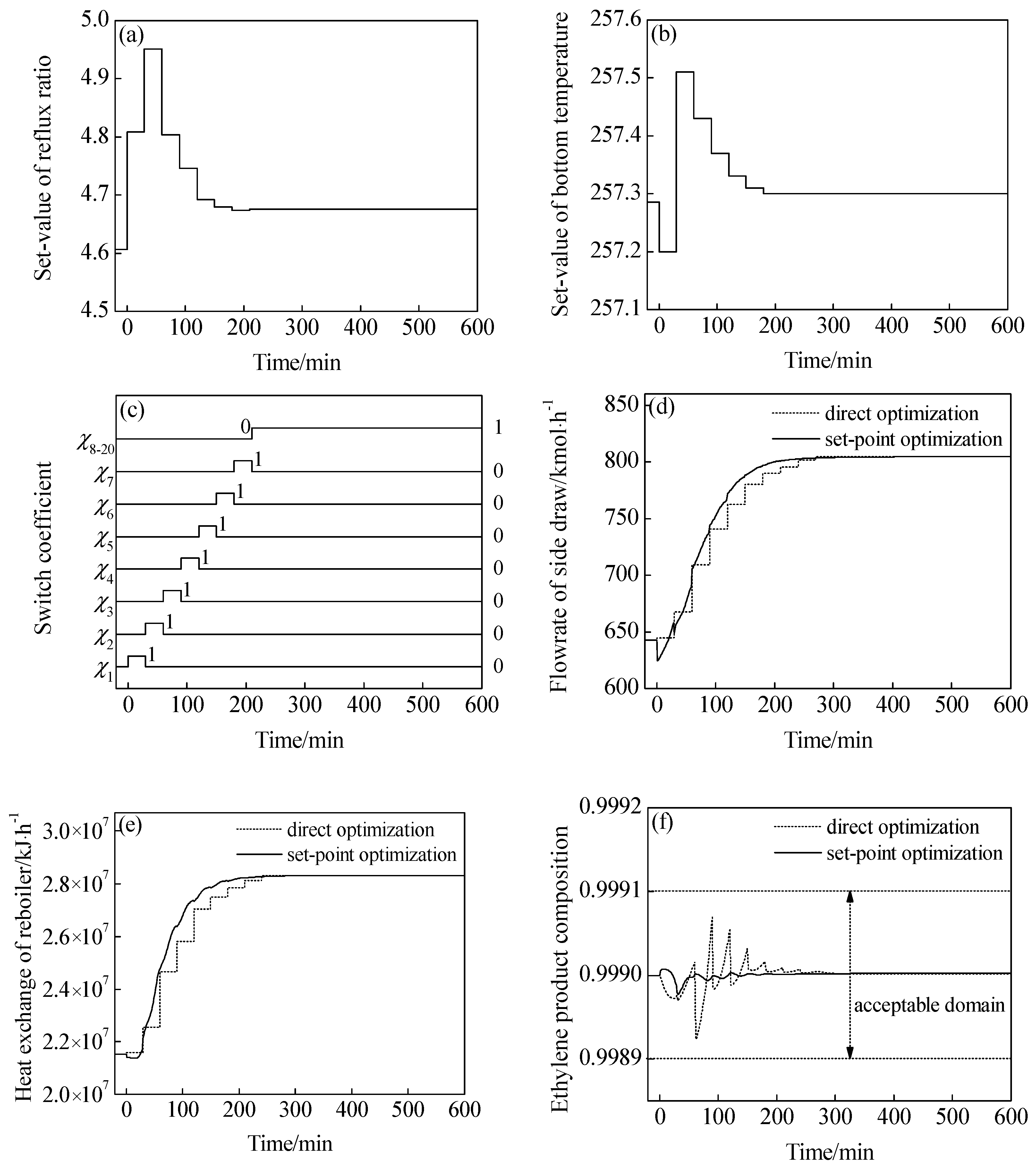
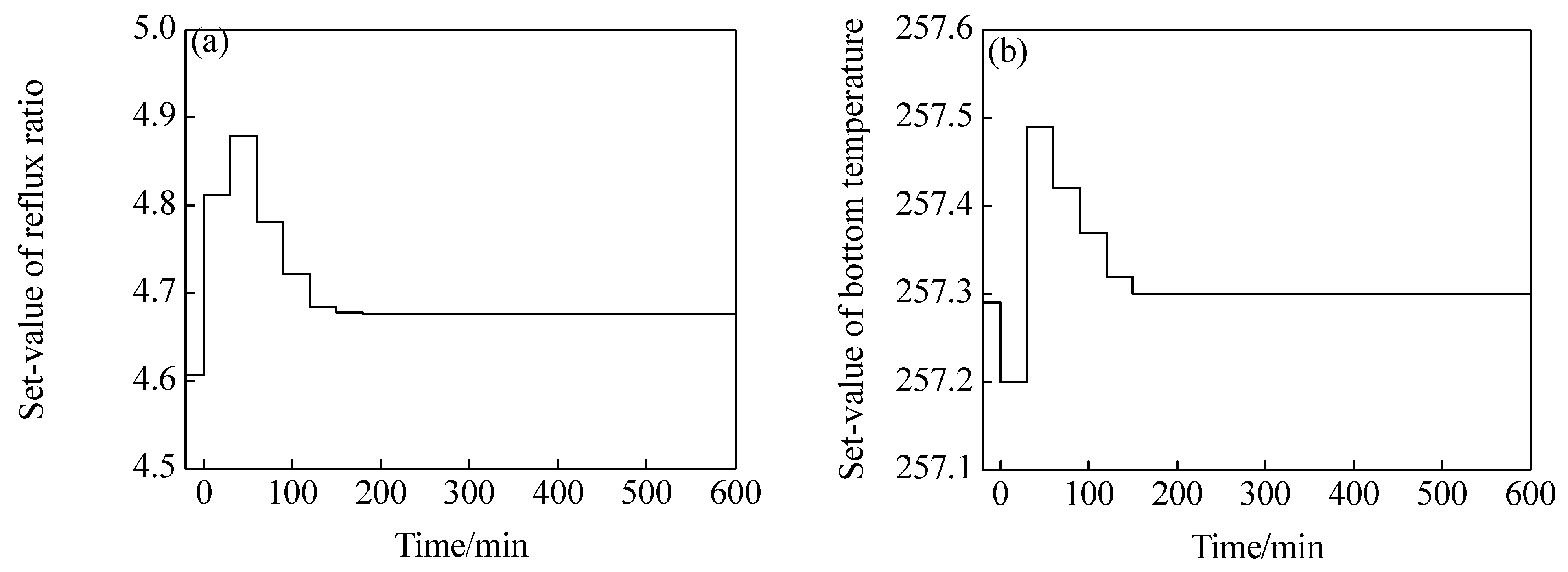
5.1. Process Transition Based on Set-Point Optimization

Dynamic optimization is recommended to search for a feasible trajectory, whereas the target of dynamic optimization is to reduce the fluctuation of ethylene product quality during the process transition. To avoid the structural adjustment that leads to process unsteadiness, an approach to process transition via regulatory controllers, namely set-point optimization, is proposed.

For simulation, the set-point controllers are established by the ready module. Moreover, the proportion and integration parameters are given by the practical operation. The set-point optimization is solved by two steps of the equal time-interval approach.

The first step is providing the discrete time grid. The control horizon and the discrete periodic are, respectively, assigned as 600 min and 30 min from experience; a detailed demonstration has been given in the previous research of the authors [2]. That is to say, the control horizon consists of a 20-time grid, whose interval is 30 min. The B-splines function is assigned as

$${\chi }_k(t)=\left\{\begin{array}{cc}1& \mathrm{if}\begin{array}{c} \end{array}30(k-1)\le t<30k\\ 0& \mathrm{else}\end{array}\right.\begin{array}{cc}, & k=1, 2, 3, \cdots , 20.\end{array}$$

(29)

While the discrete time grid is given, the decision variables of the problem are the sequences of optimization variables of set-point optimization in all time intervals, namely ${\widehat{\mathit{R}}}_{\mathbf{s}\mathbf{p}}$ and ${\widehat{\mathit{T}}}_{\mathbf{s}\mathbf{p}}$.

The second step is solving the NLP problem. The optimal sequences of optimization variables are shown in

Table 2. Optimal result of set-point optimization.

Time Interval	Duration (min)	Reflux Ratio Set-Value	Bottom Temperature Set-Value (K)
Initialization (0)	--	4.606	257.29
1	30	4.809	257.20
2	30	4.951	257.51
3	30	4.804	257.43
4	30	4.746	257.37
5	30	4.692	257.33
6	30	4.680	257.31
7	30	4.674	257.30
8–20	390	4.676	257.30

.

Based on the optimal sequences in Table 2, the trajectory of optimization variables is shown in Figure 5a–c. Moreover, the trajectory of manipulated variables and product quality of the ethylene column is drawn in Figure 5d–f.

Figure 5a,b are the optimal trajectory of optimization variables, namely the connection of the optimal sequence in Table 2 to the timeline. Figure 5c is the trajectory of the B-spline function, which determines the discrete time grid. For direct optimization, the optimal sequences of manipulated variables, which contain the molar flowrate of the side draw and the heat flowrate of the reboiler, are calculated and shown as the dashed line in Figure 5d,e. The ethylene quality is manipulated by the discrete sequences and shown as the dash line in Figure 5f. For set-point optimization, the discrete sequences of controller input variables, which contain the set-value of reflux ratio and bottom temperature controllers, are softened and shown as the solid line in Figure 5d,e. The trajectory of ethylene quality is shown as the solid line in Figure 5f.

On the basis of the comparison in Figure 5d–f, the step change of manipulated variables is avoided by the employment regulatory controllers, and the curve is smoothed for flowrate of side draw and heat exchange of the reboiler. The softness of manipulated variables reduces the fluctuation of the ethylene product. In detail, the results are displayed in

Table 3. Simulation results for different types of optimization.

Performance	Direct Optimization	Set-Point Optimization
Effective control horizon (min)	270	210
IAE of product quality (10−3)	2.424	1.093
Maximum deviation of product quality (10−4)	0.685	0.181

.

As shown in Table 3, for set-point optimization, the effective control horizon, namely the duration before the ethylene quality is stabilized, is shortened, and the ethylene quality fluctuation is significantly reduced. That is to say, the involvement of set-point controllers is beneficial to improving the performance of dynamic optimization. In a word, the approach to process transition via regulatory controllers not only avoids the insecurity and instability caused by the switching of set-point controllers but also improves the control performance.

5.2. Tunable Controller Parameters

The advantage of set-point optimization is proven in Section 3.2 and verified in Section 5.1. There is a factor that affects the performance of set-point optimization. In general, although the switching of control structure and control algorithm is not recommended for continuous production, the control parameters could be adjusted. The influence of set-point controllers’ parameters on control performance is due to the change in the equivalent filter’s transfer function. While the control parameters are tunable, the optimization vector is extended as Equation (30).

$${\mathit{u}}_{\mathbf{s}\mathbf{p}}(\mathit{t})={\left[\begin{array}{cc}{\mathit{x}}_{\mathbf{s}\mathbf{p}}(\mathit{t})& {\mathit{p}}_{\mathbf{c}}(t)\end{array}\right]}^{\mathrm{T}}$$

(30)

where ${\mathit{u}}_{\mathbf{s}\mathbf{p}}$ is the extended optimization vector for set-point optimization; ${\mathit{p}}_{\mathbf{c}}$ is the control parameters, which contain the proportion and integration of set-point controllers. While the proportion of reflux ratio controllers is discussed, the optimal sequences of optimization variables are shown in

Table 4. Optimal result of set-point optimization with a tunable control parameter.

Time Interval	Duration (min)	Reflux Ratio Set-Value	Bottom Temperature Set-Value (K)	Proportion of Reflux Ratio Controller
Initialization (0)	--	4.606	257.29	0.361
1	30	4.812	257.20	0.158
2	30	4.879	257.49	0.143
3	30	4.781	257.42	0.234
4	30	4.722	257.37	0.251
5	30	4.685	257.32	0.263
6	30	4.678	257.30	0.268
7–20	420	4.676	257.30	0.271

.

Based on the optimal sequences in Table 4, the trajectory of optimization variables is shown in Figure 6a–c. Moreover, the trajectory of manipulated variables and product quality of the ethylene column is drawn in Figure 6d–f.

Figure 6a–c are the optimal trajectory of optimization variables, whereas Figure 6d,f are the optimal trajectory of manipulated variables. Based on the comparison in Figure 6f, the adjustment of the control parameter reduces the fluctuation of the ethylene product. In detail, the results are displayed in

Table 5. Simulation results for different control parameters.

Performance	Direct Optimization	Set-Point Optimization
Effective control horizon (min)	210	180
IAE of product quality (10−3)	1.093	0.953
Maximum deviation of product quality (10−4)	0.181	0.154

.

As shown in Table 5, the control performance of the process transition is slightly improved by the adjustment of the set-point controller’s parameter. Despite operation complexity increasing, optimization of control parameters is an effective way to further improve control performance.

6. Conclusions

Dynamic optimization is a suitable approach to implement the process transition for a continuous chemical process. This paper discusses the influence of regulatory controllers on dynamic optimization and proposes two types of dynamic optimization models, namely direct optimization and set-point optimization. To avoid the operation insecurity caused by the adjustment of the regulatory control structure, set-point optimization is recommended. What is more, the merit of set-point optimization is rigorously proven for general situations.

By simulation, the process transition of a throughput-fluctuation ethylene column, caused by the decoking of a cracking furnace, is implemented by set-point optimization. Comparing with direct optimization (the previous work of the authors), the involvement of set-point controllers is beneficial to improving the performance of dynamic optimization. In a word, the approach to process transition via regulatory controllers not only avoids the insecurity caused by the switching of set-point controllers but also improves the control performance. In addition, the influence of adjusting set-point controllers’ parameters on optimization performance is positive.

References

1. Xie, Y.F.; Liu, J.H.; Xu, D.G.; Gui, W.H.; Yang, C.H. Optimal control strategy of working condition transition for copper flash smelting process. Contr. Eng. Pract. 2016, 46, 66–76. [Google Scholar] [CrossRef]
2. Huang, D.; Luo, X.L. Process transition based on dynamic optimization with the case of a throughput-fluctuating ethylene column. Ind. Eng. Chem. Res. 2018, 57, 6292–6302. [Google Scholar] [CrossRef]
3. Cao, X.Y.; Xu, F.; Luo, X.L. A novel strategy of continuous process transition and wide range throughput fluctuating ethylene column. J. Taiwan Ins. Chem. Eng. 2021, 121, 61–73. [Google Scholar] [CrossRef]
4. Yang, C.; Wang, K.X.; Shao, Z.J.; Biegler, L.T. Integrated parameter mapping and real-time optimization for load changes in high-temperature gas-cooled pebble bed reactors. Ind. Eng. Chem. Res. 2018, 57, 9171–9184. [Google Scholar] [CrossRef]
5. Victor, D.; Sergey, S. Electrically controlled optical spectral filters for WDM communication networks based on multilayer inhomogeneous holographic diffraction structures. In Proceedings of the IX International Conference on Information Technology and Nanotechnology (ITNT), Samara, Russian, 17–21 April 2023. [Google Scholar]
6. Rabii, A.; El Sayed, A.; Ismail, A.; Aldin, S.; Dahman, Y.; Elbeshbishy, E. Optimizing the Mixing Ratios of Source-Separated Organic Waste and Thickened Waste Activated Sludge in Anaerobic Co-Digestion: A New Approach. Processes 2024, 12, 794. [Google Scholar] [CrossRef]
7. Tatjewski, P. Advanced control and on-line process optimization in multilayer structures. Annu. Rev. Contr. 2008, 32, 71–85. [Google Scholar] [CrossRef]
8. Delou, P.D.A.; Curvelo, R.; Maurício, B.; Secchi, A.R. Steady-state real-time optimization using transient measurements in the absence of a dynamic mechanistic model: A framework of HRTO integrated with Adaptive Self-Optimizing IHMPC. J. Process Contr. 2021, 106, 1–19. [Google Scholar] [CrossRef]
9. Li, X.X.; Yang, J.M.; Sun, H.; Che, H.J.; Hu, Z.Y.; Zhao, Z.W. Inverse model based prediction for evolutionary dynamic multiobjective optimization. In Proceedings of the Chinese Automation Congress (CAC), Shanghai, China, 6–8 November 2020. [Google Scholar]
10. Liang, E.; Yuan, Z. Robust dynamic optimization for nonlinear chemical processes under measurable and unmeasurable uncertainties. AIChE J. 2022, 8, 17733. [Google Scholar] [CrossRef]
11. Soloveva, O.V.; Solovev, S.A.; Shakurova, R.Z. Numerical Study of the Thermal and Hydraulic Characteristics of Plate-Fin Heat Sinks. Processes 2024, 12, 744. [Google Scholar] [CrossRef]
12. Dirza, R.; Matias, J.; Skogestad, S.; Krishnamoorthy, D. Experimental validation of distributed feedback-based real-time optimization in a gas-lifted oil well rig. Contr. Eng. Pract. 2022, 126, 105253. [Google Scholar] [CrossRef]
13. Lv, K.; Liu, H.; Liu, X.; Zhou, Y.; Jiang, W.; Zheng, W. Numerical analysis and differential push-flow structure optimization of vacuum disc drying process. Can. J. Chem. Eng. 2023, 12, 6845–6857. [Google Scholar] [CrossRef]
14. Esche, E.; Arellano-Garcia, H.; Wozny, G.; Biegler, L.T. Optimal operation of a membrane reactor network. AIChE J. 2014, 60, 1321–1325. [Google Scholar] [CrossRef]
15. Oliveira, R.D.; Roux, G.A.; Mahadevan, R. Nonlinear programming reformulation of dynamic flux balance analysis models. Compu. Chem. Eng. 2023, 170, 108101. [Google Scholar] [CrossRef]
16. Liu, X.G.; Hu, Y.Q.; Feng, J.H.; Liu, K.A. A Novel penalty approach for nonlinear dynamic optimization problems with inequality path constraints. IEEE Trans. Automat. Contr. 2014, 59, 2863–2867. [Google Scholar] [CrossRef]
17. Wang, L.W.; Liu, X.G.; Zhang, Z.Y. A new sensitivity-based adaptive control vector parameterization approach for dynamic optimization of bioprocesses. Bioprocess Biosyst. Eng. 2017, 40, 181–189. [Google Scholar] [CrossRef]
18. Zhang, K.; Wu, X.; Lin, J.; Cheng, M. Sensitivity analysis for the optimization of switched dynamical processes with state-dependent switching conditions and its application. J. Ind. Manag. Optim. 2023, 10, 7306–7333. [Google Scholar]
19. Ko, D. Conceptual design optimization of an integrated membrane bioreactor system for wastewater treatment. Chem. Eng. Res. Des. 2018, 132, 385–398. [Google Scholar] [CrossRef]
20. Almasi, A.; Yavari, L.; Mohammadi, M.; Mousavi, S.A. Optimization of an integrated system for refinery wastewater treatment. Toxin Rev. 2020, 39, 408–421. [Google Scholar] [CrossRef]
21. Adetola, V.; Guay, M. Integration of real-time optimization and model predictive control. J. Process Contr. 2010, 20, 125–133. [Google Scholar] [CrossRef]
22. Jia, M.X.; Chen, C.H.; Kou, W.Q.; Niu, D.P.; Wang, F.L. Real-time optimization of converter inlet temperature in acid production with flue gas. Chem. Eng. Res. Des. 2017, 122, 226–232. [Google Scholar] [CrossRef]
23. Li, Z.; Wang, X.; Kruger, U. Efficient cross-validatory algorithm for identifying dynamic nonlinear process models. Contr. Eng. Pract. 2021, 111, 104787. [Google Scholar] [CrossRef]
24. Cheng, Z.; Tenny, K.; Pizzolato, A.; Forner-Cuenca, A.; Verda, V.; Chiang, Y.M. A generalized reduced fluid dynamic model for flow fields and electrodes in redox flow batteries. AIChE J. 2022, 4, 17540. [Google Scholar] [CrossRef]
25. Asad, H.S.; Yuen, R.K.K.; Huang, G.S. Multiplexed real-time optimization of HVAC systems with enhanced control stability. Appl. Energy 2017, 187, 640–651. [Google Scholar] [CrossRef]
26. Zhou, H.L.; Chen, X.; Wu, M.; Cao, W.H.; Hu, J. A new hybrid modeling and optimization algorithm for improving carbon efficiency based on different time scales in sintering process. Contr. Eng. Pract. 2019, 91, 104104. [Google Scholar] [CrossRef]
27. Luo, Y.; Gopaluni, B.; Cao, L.; Wang, Y.J.; Cheng, J. Adaptive online optimization of alarm thresholds using multilayer Bayesian networks and active transfer entropy. Contr. Eng. Pract. 2023, 137, 105534. [Google Scholar] [CrossRef]
28. Dirza, R.; Skogestad, S. Primal–dual feedback-optimizing control with override for real-time optimization. J. Process Contr. 2024, 138, 103208. [Google Scholar] [CrossRef]
29. Marco, V.; Riccardo-Bacci, D.C.; Elisabetta, B.; Leonardo, T.; Paolo, P.; Roberto, V.; Gabriele, P. Optimally managing chemical plant operations: An example oriented by industry 4.0 paradigms. Ind. Eng. Chem. Res. 2021, 21, 7853–7867. [Google Scholar]
30. Nie, Y.; Kerrigan, E.C. Solving dynamic optimization problems to a specified accuracy: An alternating approach using integrated residuals. IEEE Trans. Automat. Contr. 2023, 68, 548–555. [Google Scholar] [CrossRef]
31. Jie, H.; Zhu, G.Z.; Hong, W.R. Direct approaches for PDE-constrained dynamic optimization based on space–time orthogonal collocation on finite elements. J. Process Contr. 2023, 124, 187–198. [Google Scholar] [CrossRef]
32. Turan, E.M.; Jäschke, J. Closed-loop optimisation of neural networks for the design of feedback policies under uncertainty. J. Process Contr. 2024, 133, 103144. [Google Scholar] [CrossRef]
33. Huang, D.; Luo, X.L. A novel approach to promptly control product quality in precise distillation columns based on pressure dynamic modeling. Asia-Pac. J. Chem. Eng. 2018, 13, e2212. [Google Scholar] [CrossRef]
34. Huang, D.; Zhao, X.Y.; Luo, X.L. Trade-off between energy consumption and ethylene recovery rate for quasi-plant wide operation optimization of the ethylene column with bottom circulatory system in ethylene complex. Asia-Pac. J. Chem. Eng. 2017, 12, 694–708. [Google Scholar] [CrossRef]
Figure 1. Process transition under the multilayer control structure.
Processes 12 01105 g001
Figure 2. Control structures for different optimization types: (a) direct optimization; (b) set-point optimization.
Processes 12 01105 g002
Figure 3. Comparison between direct optimization and set-point optimization ((a). direct optimizaiton structure; (b). set-point optimization structure; (c). intermediate set-point optimization structure; (d). final set-point optimization structure).
Processes 12 01105 g003
Figure 4. Diagram of the ethylene column and regulatory control system.
Processes 12 01105 g004
Figure 5. Optimal trajectory for set-point optimization: (a) reflux ratio set-value; (b) bottom temperature set-value; (c) spline function; (d) molar flowrate of side draw; (e) heat flowrate of reboiler; (f) ethylene product quality.
Processes 12 01105 g005
Figure 6. Optimal trajectory with a tunable control parameter: (a) reflux ratio set-value; (b) bottom temperature set-value; (c) spline function; (d) molar flowrate of side draw; (e) heat flowrate of reboiler; (f) ethylene product quality.
Processes 12 01105 g006aProcesses 12 01105 g006b