Study of Draft Tube Optimization Using a Neural Network Surrogate Model for Micro-Francis Turbines Utilized in the Water Supply System of High-Rise Buildings

Abstract

With the increasing popularity of clean energy, the use of micro turbines to recover surplus energy in the water supply pipelines of high-rise buildings has attracted more attention. This study adopts a predictor model based on Radial Basis Function Neural Network (RBFNN) to optimize the draft tube shape for micro-Francis turbines. The predictor model is formed on a dataset provided by numerical simulations, which are validated by lab tests. Specifically, numerical investigations are carried out in the shape of a draft tube to determine an optimal model. Additionally, the superiority of the RBFNN model in nonlinear optimization is verified by comparing it with other models under the same date sets. After that, the design parameters are optimized using RBFNN and sequential quadratic programming algorithm (SQPA). Finally, the turbine prototype is fabricated and tested on a lab test rig. The experimental results indicate that the numerical method adopted in this research is accurate enough for such a micro-Francis turbine performance prediction. Under the design conditions, the proposed micro-Francis turbine produces a power of 147 W with an efficiency of over 29%, which shows a considerable improvement compared to the initial prototype.

1. Introduction

With the progress of urbanization, the number of high-rise buildings in cities has been increasing significantly [1,2], which also leads to a huge energy consumption in the urban water supply systems (WSS) [3,4]. In order to supply water to high-rise buildings, the secondary water supply equipment is usually employed [5]. Before supplying water to the buildings, pressure-reducing valves (PRVs) are commonly used to minimize leakages and damages caused by high-pressure water flow from the municipal network [6,7]. However, the PRV may reduce the energy efficiency of WSS as it achieves water head reduction by dissipating excess energy. By contrast, micro turbines can not only convert excess water energy into electrical energy, but also can recover the excess energy in the pipeline [8,9]. Therefore, the replacement of PRVs with micro-hydro turbines is a promising solution to reduce the water supply energy consumption of buildings.

As a traditional type of pressure turbine, the Francis turbine can maintain high efficiency over a wide range of water head and flow rate, so it is widely used in micro, medium, and large hydropower plants [10]. And, the Francis turbine is more suitable for closed systems where downstream water pressure is required [11]. Some scholars have carried out research related to the micro application of Francis turbines. Xiong et al. [12] developed a micro-Francis turbine with an inlet and outlet diameter of 40 mm based on the single-factor design theory. Simulation results showed that at a rotational speed of 1200 r/min and an inlet flow rate of 3.47 × 10⁻³ m³/s, the water turbine had a water head of 8.1 m, an output power of 135 W, and an efficiency of 48.5%. Guo et al. [13] designed a micro-Francis turbine for a 15 mm diameter water pipe with a flow velocity range of 1–3 m/s for converting the excess hydraulic energy in the pipe to supply the induction faucet. After optimization with orthogonal experiments setting the internal pipe flow velocity to 1.5 m/s and the available water head to 3 m, the output power of the Francis turbine was 6.3 W, and the efficiency was 85.13%. Experimental results showed that the output power of the generator was 6.35 W at the set flow rate, and the total system efficiency was 85.8%. Another study [6] showed that it is feasible to apply a single-stage pump-turbine for excess water energy recovery in the WSS of buildings. The micro-Francis turbine is similar to the single-stage pump-turbine in terms of structural composition and water flow status inside the equipment during operation [14]. Based on the above research, it is feasible to recover excess hydraulic energy in the WSS by applying a micro-Francis turbine.

As the flow passage component of the Francis turbine, the draft tube is usually located below the runner. The main functions of the draft tube include directing the flow of water from the runner outlet to the downstream and recovering energy. As a core component of Francis turbines, the draft tube has a significant impact on the performance of the turbine. Therefore, the design theory and optimization methods of the draft tube have been a major research focus. Tania et al. [15] used three types of curves and their combinations to define the influence of the geometry of the draft tube elbow profile on the performance of Francis turbines. The study found that the hyperbolic–logarithmic form of draft tube had the highest efficiency, while the logarithmic form of draft tube had the lowest loss coefficient. Chen et al. [16] introduced the J-shaped groove technology on the wall of the draft tube to expand the operating range of Francis turbines and meet the energy demand. The optimized J-shaped groove significantly mitigated the pressure fluctuation inside the draft tube, stabilizing the operation of Francis turbines under non-design conditions. Zhou et al. [17] introduced an inclined conical diffuser into the draft tube. The results showed that at a speed of 250 r/min, the maximum pressure fluctuation amplitude of the improved draft tube reduced by 18.4% compared to that of the traditional draft tube. However, there is still limited research on the draft tube of micro-Francis turbines for pipeline applications.

Artificial neural networks are often used to generate predictive models to optimize equipment performance [18]. Numerous researchers have effectively employed neural networks for the optimization of hydraulic turbines. Hasanzadeh et al. [19] utilized artificial neural networks and multi-objective genetic algorithms to optimize runner and deflector blocks. Similarly, Mengistu et al. [20] applied an evolutionary optimization algorithm based on artificial neural networks for the aerodynamic optimization of turbine blades. Therefore, it is feasible to optimize the draft tube using neural networks to improve its performance.

This study developed a micro-Francis turbine for high-rise buildings in the WSS and introduced the RBFNN to optimize the shape of the draft tube. Unlike traditional Francis turbines, the exit of the micro-Francis turbine runner is located below the tailwater level. To align the center of the draft tube outlet with the center of the volute inlet, an “S”-shaped draft tube was designed. The structure of this paper is as follows. Section 2 describes the theoretical optimization method, design conditions of the draft tube, and the numerical simulation and lab test adopted in this study. In Section 3, numerical simulation and lab test results based on the optimal parameters are presented. Finally, the main conclusions of this study are summarized.

2. Methodology

The entire research flow chart is indicated in Figure 1. The draft tube optimization starts with the parameterization of the shape based on Bezier curves. After that, the Latin hypercube sampling and numerical simulations are used to create an initial uniform set of samples. Since RBFNN is applicable to nonlinear optimization, the nonlinear relationship between the design variables and the optimization objective is proved. Additionally, to prove the superiority of the RBFNN model in nonlinear optimization, the model errors of standard response surface functions, radial basis function and Kriging function are compared under the same date sets. And then, the acceptability of the accuracy of the RBFNN is judged, and acceptable models are used to find the optimal design parameters. If the accuracy is deemed unacceptable, additional sample points are required. Finally, the prototype is fabricated and lab tests are conducted to validate the numerical results and study the turbine performance. The design process would be repeated if the numerical or Lab test results do not satisfy the design requirements.

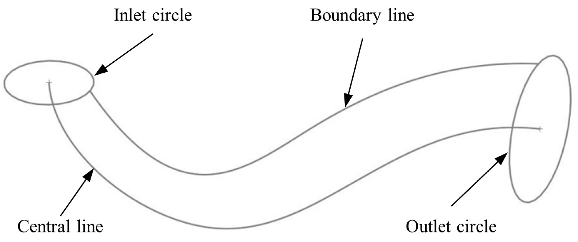
2.1. Francis Turbine Model and Modified Draft Tube

The WSS for high-rise buildings in Hong Kong was selected as the subject of the study, and the pipe diameter of this WSS is 100 mm. Based on previous studies of flow data throughout the day in this water supply pipeline [20], it can be determined that the design flow rate of the turbine would be 10 m³/h. An excessive water head may cause leakage in the WSS and damage to the water supply equipment, so the water head of fresh water needs to be reduced by 30–50 m before it enters the WSS from the municipal pipeline. The design water head of the turbine can be determined to be 30 m by combining the above analysis.

Water head H, power P and efficiency η are the most important indicators for turbine performance evaluation. Turbine power can be divided into theoretical power P_t, mechanical shaft power P_s and output power P_e. Theoretical power P_t refers to the energy of water flow utilized by the turbine, which can be calculated by Equation (2). Mechanical shaft power P_s refers to the mechanical energy captured from water flow by the runner. The output power P_e is the electrical energy output by the generator. The total efficiency η_t of the turbine is determined by the mechanical shaft conversion efficiency η_s and the generator conversion efficiency η_e together. The respective calculation formulas are as follows:

$$H=\frac{(P_{inlet}-P_{outlet})}{\rho g}$$

(1)

$$P_t=\frac{\rho gHQ}{3600}$$

(2)

$$P_s=\frac{nT}{9.55}$$

(3)

$${\eta }_s=\frac{P_s}{P_t}={\eta }_h{\eta }_l{\eta }_m$$

(4)

$$P_e={\eta }_s{\eta }_e{P}_t=\frac{{\eta }_h{\eta }_l{\eta }_m{\eta }_e\rho gHQ}{3600}$$

(5)

$${\eta }_t={\eta }_s{\eta }_e=\frac{P_e}{P_t}$$

(6)

The conventional Francis turbine structure mainly includes the volute, guide vane, runner, and draft tube. Based on the above basic requirements, the flow path structure of the Francis turbine developed in this research is shown in Figure 2. In order to reduce the installation space required for the turbine, the design does not contain a guide vane. In addition, a radial inlet volute and an “S”-shaped draft tube are used to make the center of the turbine inlet and outlet coincide with the central line of the pipe.

The turbine draft tube inlet is connected to the runner outlet, and the draft tube outlet is connected to the circular inlet of the outlet reducer, so the draft tube inlet and outlet and its cross-sectional shape are designed to be circular. The shape control of the draft tube can be achieved by controlling the shape of the central line of the draft tube and the distribution of the radius of the cross sections along the central line. The 3D modeling of the draft tube is built by SolidWorks 2016. Figure 3 shows the sketch of the shape definition of the draft tube, including the inlet and outlet circles, the central line and the boundary line. For the distribution of the radius of the section along the central line, the shape of the boundary line can be adjusted to control.

Based on the optimized design of the runner, the diameter of the runner outlet can be determined as 46 mm [21]. Therefore, the corresponding radius of the draft tube inlet is set as 23 mm. In addition, the height difference between the center of the draft tube outlet circle and the center of the volute inlet circle is 22.5 mm in order to make the center of the draft tube outlet and the center of the inlet circle coincide.

By taking the center of the inlet circle of the draft tube as the origin, the shape control of the central line and boundary line is achieved by using a Bezier curve (as shown in Figure 4). Specifically, six shape control points are defined for the central line of the draft tube, and the fifth-degree Bezier curve is utilized to control them. Additionally, four shape control points are defined for the boundary line, and the third-degree Bezier curve is used to control them. The definitions of the fifth-degree and third-degree Bezier curves are as follows:

$$\begin{array}{ll}B(t)=& P_0{(1-t)}^5+5P_{1}t{(1-t)}^4+10P_2{t}^2{(1-t)}^3\\ & +10P_3{t}^3{(1-t)}^2+5P_4{t}^4(1-t)+P_5{t}^5,t\in [0,1]\end{array}$$

(7)

$$B(t)=P_0{(1-t)}^3+3P_{1}t{(1-t)}^2+3P_2{t}^2(1-t)+P_3{t}^3,t\in [0,1]$$

(8)

Based on the known conditions, P₀, Y₅ and P₆ can be determined first. For P₁ and P₄, the main purpose is to make the transition between the inlet and outlet section of the draft tube smooth, so P₀ and P₁ have the same horizontal coordinates and P₄ and P₅ have the same vertical coordinates. In addition, Y₁ is set to −50 and X₄ is set to X₅ − 40. Based on the above analysis, the unknown variables for central line shape control include X₂, Y₂, X₃, Y₃, X₅, and the unknown variables for boundary line shape control include X₇, Y₇, X₈, Y₈, Y₉, totaling 10 unknown variables.

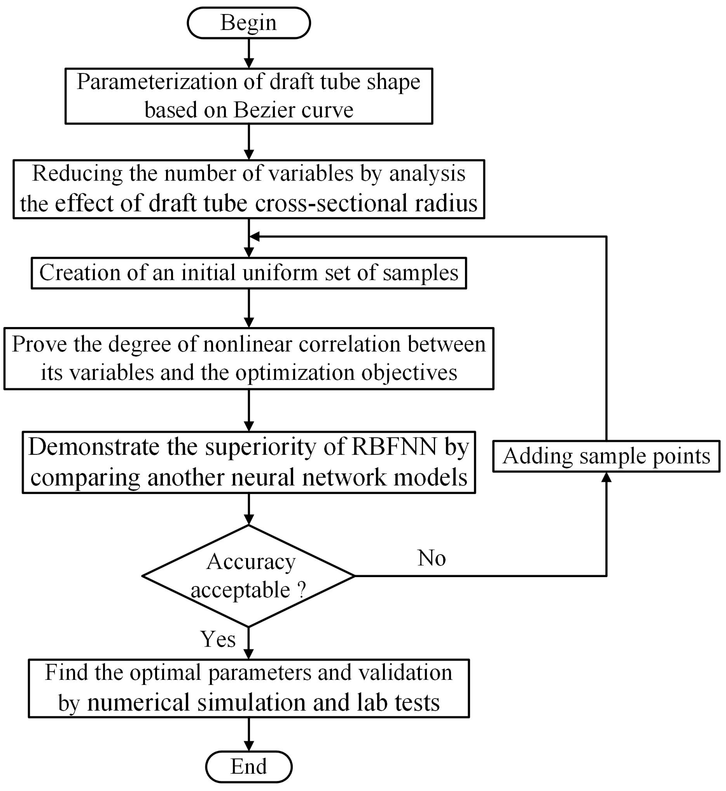
2.2. Research Methods of Draft Tube

In the process of sample collection, the sample points are selected in the design space, and the response values of the samples are obtained through numerical simulation. The sample points and their response values constitute the sample point information. The commonly used methods for sample point collection include a full factorial design, orthogonal experimental design, central composite design, Box–Behnken design, and Latin hypercube sampling. In this study, the method of Latin hypercube sampling was adopted, which can evenly and smoothly distribute the selected sample points in the design space.

RBFNN has the advantage of strong nonlinear approximation capability, so it is important to determine the nonlinear relationship between design variables and optimization objectives. The Pearson correlation coefficient r can be used to measure the degree of correlation between two sets of data. It is calculated based on the deviation of each set of data from its mean value and reflects the linear correlation between the two variables by multiplying the two deviations [22]. For two variables X = [x₁, x₂, x₃, …, x_n]^T and Y = [y₁, y₂, y₃, …, y_n]^T, the Pearson correlation coefficient r is calculated as follows [23]:

$$r=\frac{{\displaystyle {\sum }_{i=1}^n\left(x_i-\overline{x}\right)\left(y_i-\overline{y}\right)}}{\sqrt{{\displaystyle {\sum }_{i=1}^n{\left(x_i-\overline{x}\right)}^2}}\sqrt{{\displaystyle {\sum }_{i=1}^n{\left(y_i-\overline{y}\right)}^2}}}$$

(9)

where $\overline{x}$and $\overline{y}$ represent the mean values of two sets of data. The correlation coefficient r ranges from −1 to 1, where r is positive if there is a positive linear correlation between two variables, and negative if there is a negative linear correlation. Moreover, the closer the absolute value of r is to 1, the higher the degree of linear correlation between the two variables, while the closer the absolute value of r is to 0, the lower the degree of linear correlation between the two variables.

Commonly used surrogate models include standard response surface functions, Kriging functions, radial basis functions, etc. As one of the neural network agent models, the RBFNN, which is widely used due to its excellent approximation capability and faster learning speed, is a three-layer feedforward network consisting of an input layer, a hidden layer, and an output layer, with the structural features shown in Figure 5. The input layer imports m input parameters into the model in the form of vectors X = [x₁, x₂, x₃, …, x_n]^T, which are nonlinearly transformed by the hidden layer neurons and then linearly transformed by the output layer to finally obtain an output vector Y = [y₁, y₂, y₃, …, y_n]^T consisting of n responses [24]. The output response is calculated as follows [25,26]:

$$\tilde{y}={\displaystyle \sum _{i=1}^k{\alpha }_i\phi (r_i,c)}$$

(10)

where r_i is the distance between the point to be measured and the sample point; c is the control parameter; φ(r_i, c) is the basis function; α_i is the weighting factor of the ith basis function; and k is the number of basis functions.

In order to verify the superiority of the radial basis function in this study, the model errors of standard response surface functions and Kriging function can be compared under the same date sets. The response functions of standard response surface functions and Kriging function are Equations (11) and (12). Commonly used metrics for surrogate model error analysis include coefficient of determination R², root mean square error (RMSE), and maximum relative error (MRE), which are calculated by the following Equations (13)–(15) [26,27]:

Standard response surface functions:

$${\tilde{y}}_1(x)={\beta }_0+{\displaystyle \sum _{i=1}^N{\beta }_i{x}_i}+{\displaystyle \sum _{i=1}^N{\beta }_{ii}{x}_i^2}+{\displaystyle \sum _{i=2}^N{\displaystyle \sum _{j=1}^{i-1}{\beta }_{ij}{x}_i}}{x}_j$$

(11)

where N is the number of design variables; x_i, x_j are the design variables; and β₀, β_i, β_ii, β_ij are the coefficients to be determined for the polynomial.

The Kriging function is as follows:

$${\tilde{y}}_2(x)={\displaystyle \sum _{i=1}^m{\gamma }_i{f}_i(x)}+Z(x)$$

(12)

where m is the number of basis functions; f_i(x) is the determined polynomial basis function; γ_i is the weighting factor to be determined; and Z(x) is the random distribution error function.

$$R^2=\frac{{\displaystyle \sum _{i=1}^n{({\widehat{y}}_i-\overline{y})}^2}}{{\displaystyle \sum _{i=1}^n{(y_i-\overline{y})}^2}}$$

(13)

$$RMSE=\sqrt{\frac{1}{n}{\displaystyle \sum _{i=1}^n{(y_i-{\widehat{y}}_i)}^2}}$$

(14)

$$MRE=\underset{i}{\max }\left[Abs(\frac{y_i-{\widehat{y}}_i}{\overline{y}})\right]$$

(15)

where n is the number of validation points; ${\widehat{y}}_i$ is the response value of the surrogate model; y_i is the response value of the numerical simulation; and $\overline{y}$ is the arithmetic mean of y_i. The coefficient of determination R² is the most important indicator for assessing the prediction accuracy of a surrogate model, and it is generally believed that the prediction results of a surrogate model are reliable when R² is greater than 0.9. The closer the R² calculation result is to 1, the higher the prediction accuracy of the surrogate model. As for the RMSE and MRE, the closer their calculation results are to 0, the more reliable the surrogate model is considered to be.

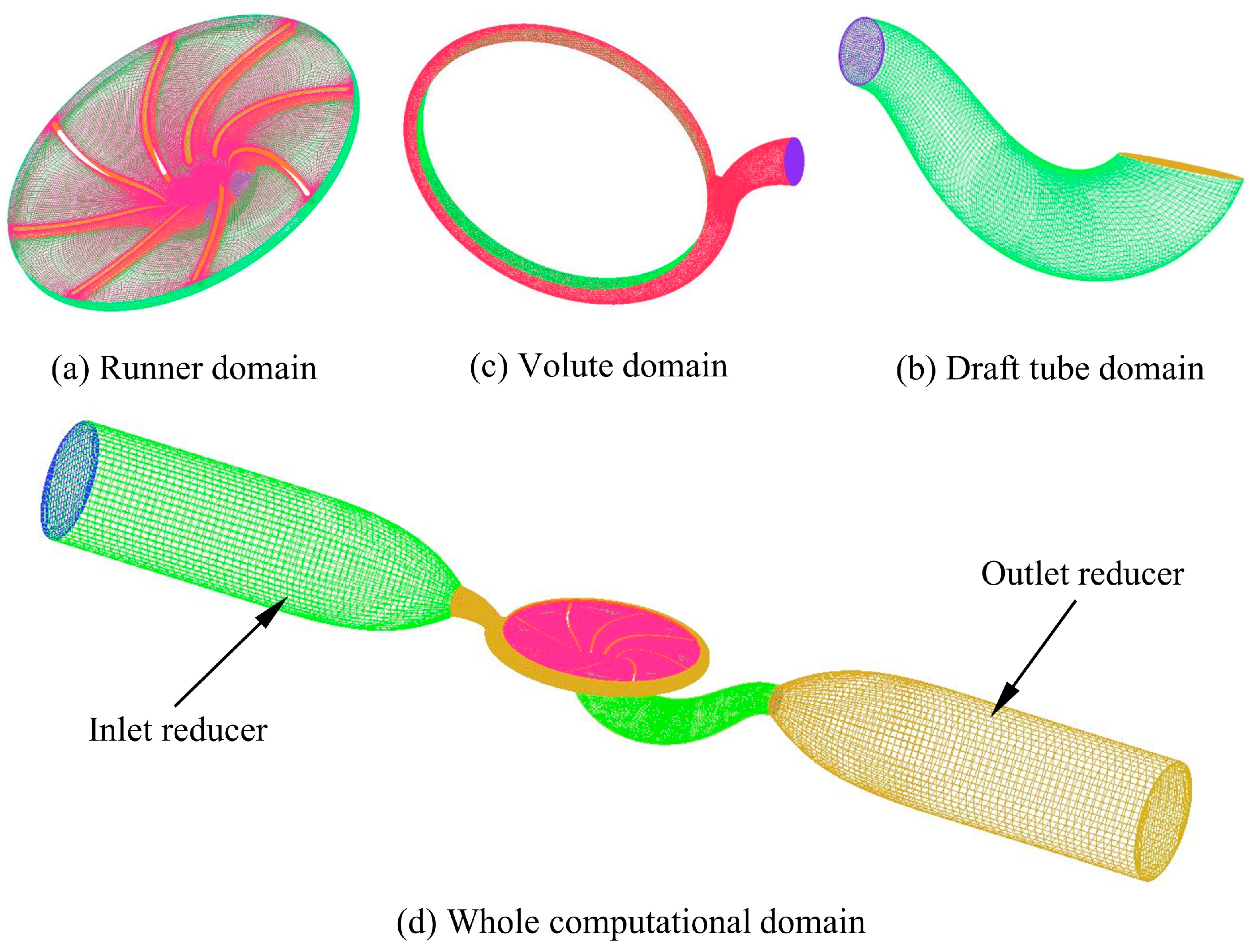
2.3. Numerical Simulation

2.3.1. Grid Generation

Ansys Turbo Grid and ICEM CFD mesh generation tools were used for model discretization. For the runner, the structured mesh is generated directly by Ansys Turbo Grid (see Figure 6a); for the draft tube, the hexahedral mesh is generated by “O” segmentation in ICEM CFD (see Figure 6b); and for the volute, the unstructured mesh is generated by ICEM CFD (see Figure 6c). In order to improve the computational accuracy, boundary layer treatment was conducted for all the wall surfaces during the meshing of different components. Figure 6 shows the meshing results. Moreover, the mesh quality of each computational domain was above 0.35, and the angle was above 18°. In addition, based on the grid independence test in the previous runner optimization study, the number of grids can be determined to be 2.29 million [21]. The final mesh model is shown in Figure 6d.

2.3.2. Simulation Settings

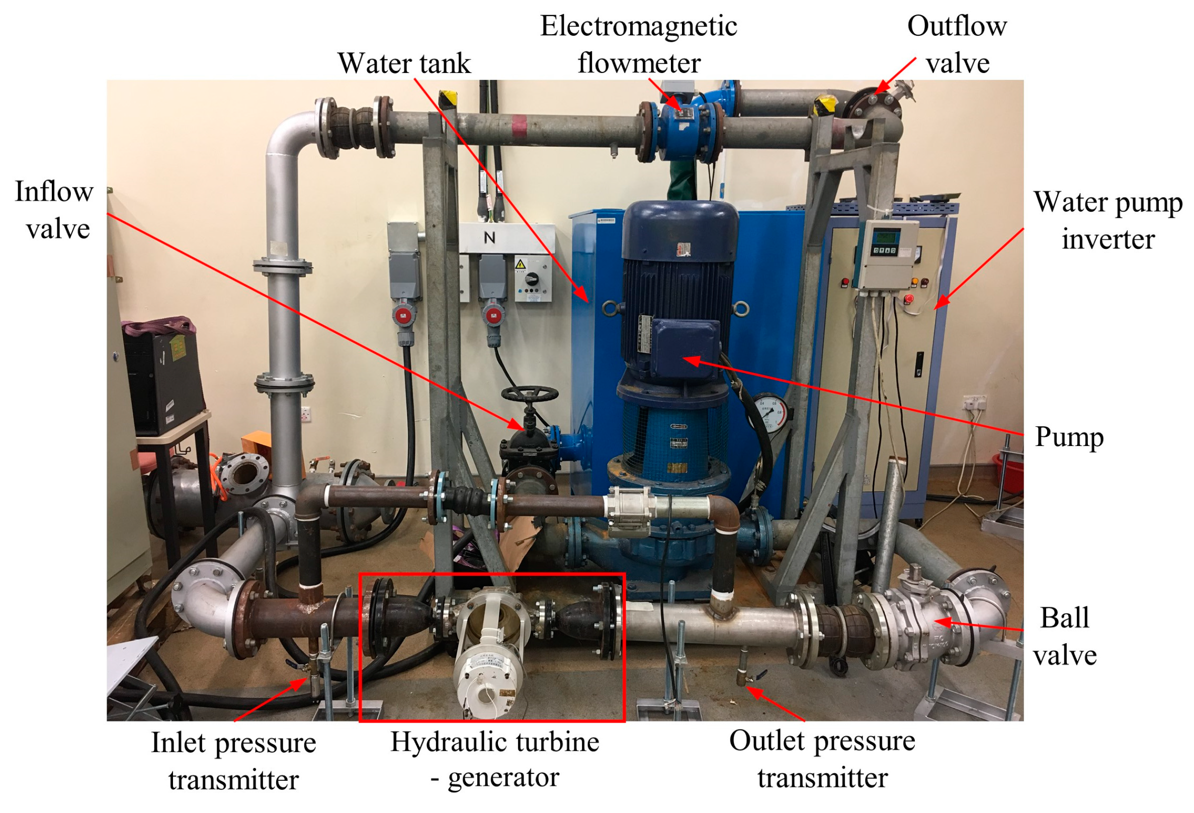
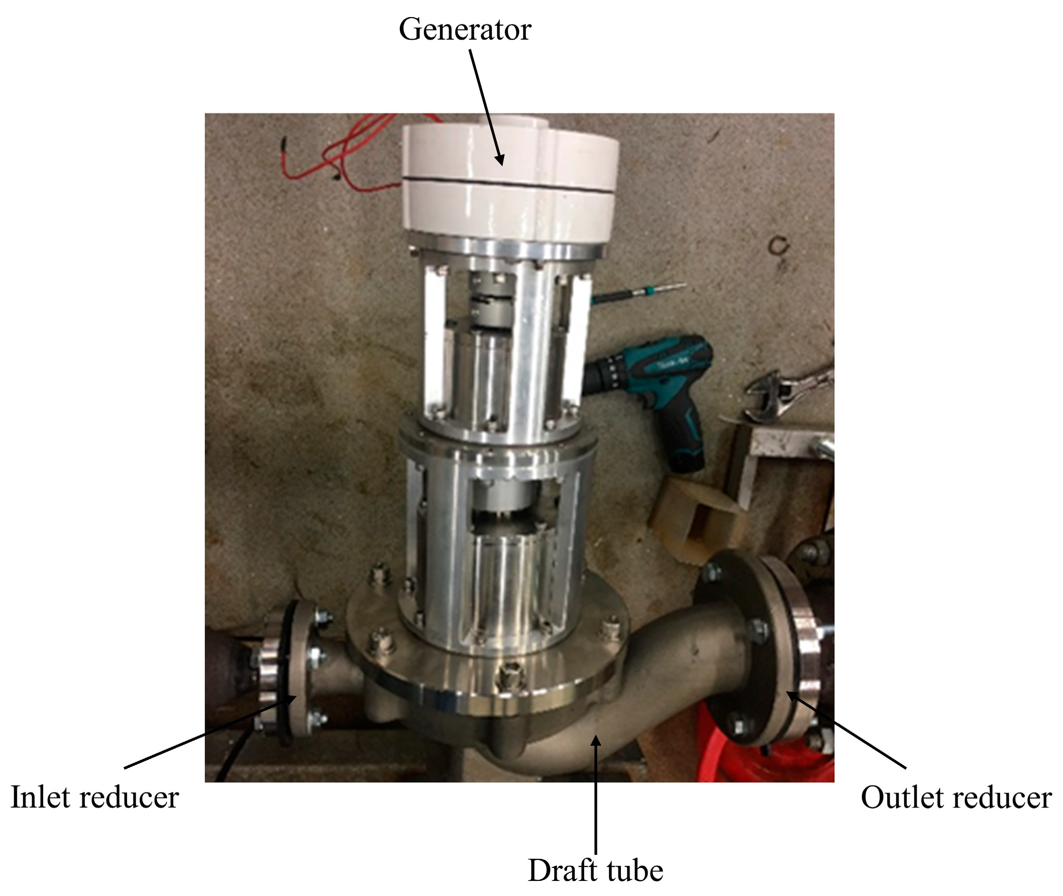
The incompressible isothermal flow through a turbomachine is fully described by the continuity and momentum equations, which are called the Navier–Stokes (N–S) equations and are written as follows [28]:

$$\frac{\partial u_i}{\partial x_i}=0$$

(16)

$$\frac{\partial u_i}{\partial t}+u_j\frac{\partial u_i}{\partial x_j}=-\frac{1}{\rho }\frac{\partial p}{\partial x_i}+\nu \frac{{\partial }^2{u}_i}{\partial x_i\partial x_j}$$

(17)

where u is the velocity, p is the pressure, v is the kinematic viscosity of fluid, and ρ is the density of water.

Since solving the Navier–Stokes equations is computationally expensive for high Reynolds number flows in complex geometries, the Reynolds averaged Navier–Stokes (RANS) equations are generally solved to determine the mean velocity field. In the numerical simulation, in order to make the control equations closed, a suitable turbulence model needs to be determined for solving the Reynolds stress. Additionally, the SST $k-\omega$ model is selected. The RANS equations are written as follows [29]:

$$\frac{\partial u_i}{\partial x_i}=0$$

(18)

$$\frac{\partial U}{\partial t}+U_j\frac{\partial U_i}{\partial x_j}=-\frac{1}{\rho }\frac{\partial p}{\partial x_i}+\frac{\partial }{\partial x_j}\left[\nu \left(\frac{\partial U_j}{\partial x_i}+\frac{\partial U_i}{\partial x_j}\right)-\rho \overline{{u^{\prime }}_i{u^{\prime }}_j}\right]$$

(19)

where U is the hourly average flow rate, and $-\rho \overline{{u^{\prime }}_i{u^{\prime }}_j}$ is the Reynolds stress.

In the process of establishing discrete equations, high-order formats are adopted for the discretization of all terms in the control equation to ensure computational accuracy. Convergence of the calculation is evaluated by considering both the variation of water head and the average residual value of the equation being less than 10⁻⁵. In the numerical simulation work, the calculation domain of the water turbine is divided into two parts: the rotating domain (runner channel) and the stationary domain (other component channels), and data transfer between the stationary and rotating domains is achieved by freezing the Frozen Rotor [30]. For the boundary and wall conditions of the model, the flow velocity is set as the inlet boundary condition of the Francis turbine, the pressure is set as the outlet boundary condition of the micro-Francis turbine, and the roughness of all walls is set to be 100 μm.

2.3.3. Lab Tests

In order to accurately obtain the real preference performance of the micro-Francis turbine after draft tube optimization and to verify the simulation results, it is also necessary to conduct lab tests using a test rig, which is shown in Figure 7. The test rig mainly includes a pump, electromagnetic flow meter, pressure transmitter, ball valve, water tank, generator, micro-Francis turbine, etc. Additionally, the test rig is driven by the pump, which has a rated flow rate of 81 m³/h and a water head of 82 m. The flow rate and water head can be measured by the electromagnetic flowmeter (accuracy ± 0.25%) and pressure transmitter, respectively. The mechanical energy captured by the turbine is converted into electrical energy using a 24 V three-phase permanent magnet AC generator. Finally, the output power of the generator is calculated by testing a 22 Ω resistor. Figure 8 shows the hydraulic test rig actually used in this project. The pipe diameter of the test rig is 100 mm, which is consistent with that of the WSS and can meet the testing requirements.

In the lab tests, the flow rate Q, the turbine inlet pressure P_inlet and the turbine outlet pressure P_outlet are measured, and the water head H and the theoretical available power P_t are calculated by Equations (1) and (2). In addition, the output power P_e is obtained in the lab tests, and the total efficiency η_t is calculated. In order to obtain P_e and η_t, the leakage efficiency η_l, the mechanical efficiency η_m and the generator conversion efficiency η_e need to be evaluated.

3. Results and Discussion

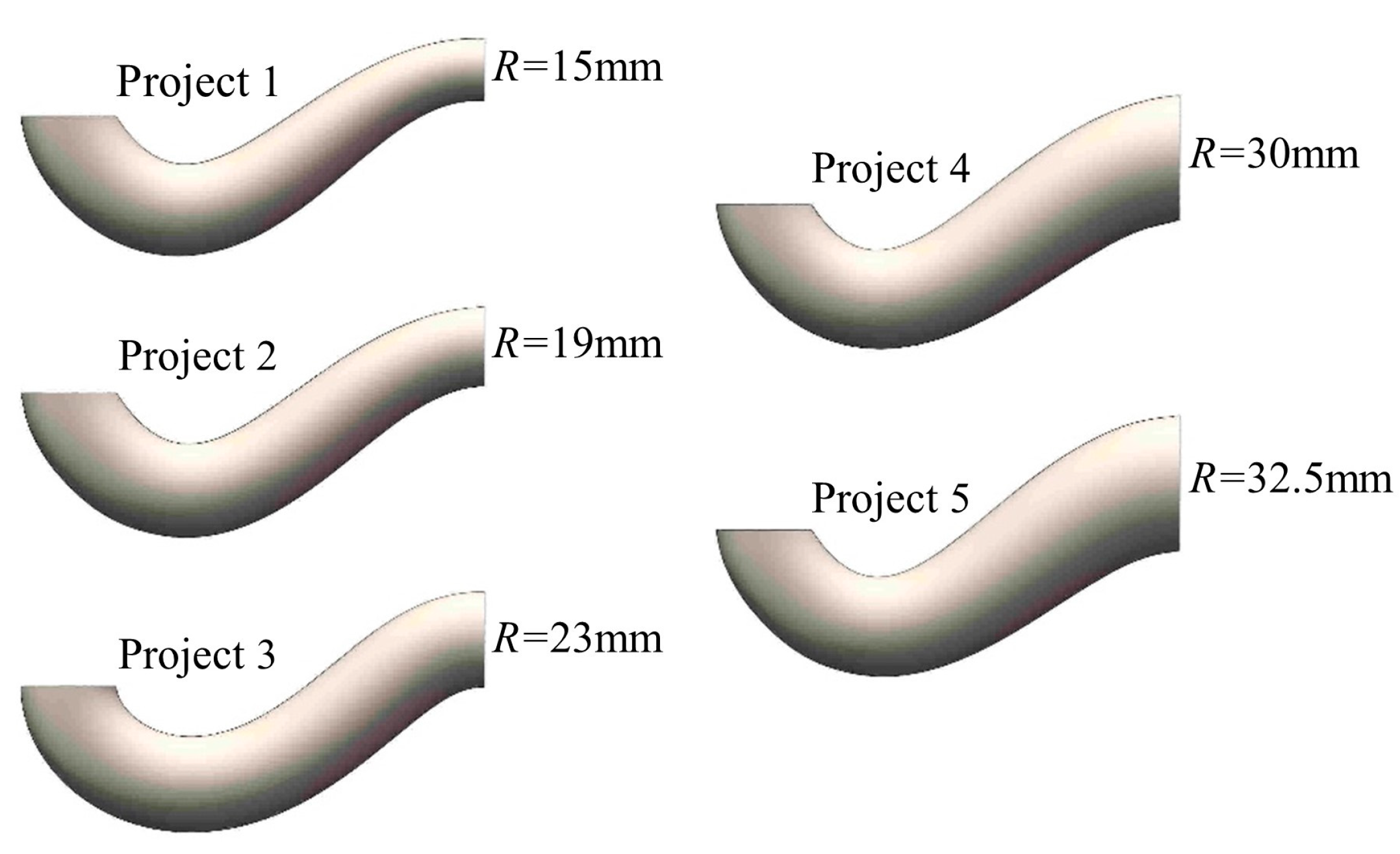
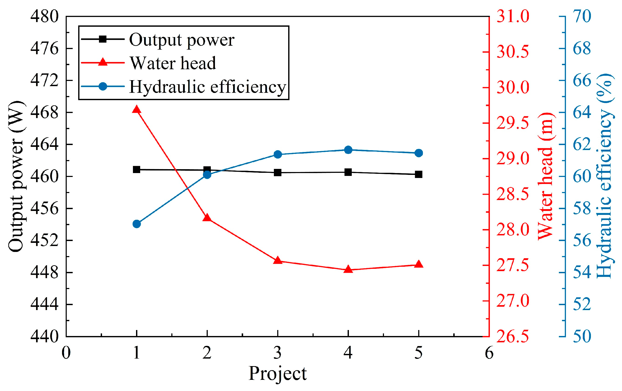
3.1. Radius Analysis of Draft Tube

The networks with fewer input numbers tend to have better accuracy. Therefore, reducing the neural network input number and finding the optimal topology for the network helps in the reduction of the network error [19]. To analyze the effect of draft tube cross-sectional radius, five different projects are built and studied. From Projects 1 to 5, the outlet radius of the draft tube gradually increased (Projects 1 and 2 were contraction-type draft tubes, Project 3 was an equal-diameter draft tube, and Project 4 and 5 were diffusion-type draft tubes). The specific values of the unknown variable for different projects are shown in

Table 1. Draft tube boundary line shape control project.

Project Number	X7	Y7	X8	Y8	Y9
Project 1	67.2	−69.2	116.7	40.5	37.5
Project 2	69.8	−72.6	114.8	38.6	41.5
Project 3	Isometric distribution (all cross-sectional radii are 23 mm)
Project 4	67.2	−69.2	116.2	46.4	52.5
Project 5	69.8	−72.6	115.6	51.9	55

, and the 3D modeling results of the draft tube of the five projects are shown in Figure 9.

The simulation results of the draft tube with different shapes under the design condition are shown in Figure 10. The hydraulic efficiency and output power are directly obtained through numerical simulations without considering leakage loss, mechanical loss, and generator conversion loss. It can be seen from the Figure 10 that for Projects 1 to 5, the water head of the turbine decreases gradually then keeping stable, while the hydraulic efficiency saw an opposite trend. Furthermore, different draft tube section radius distributions have no significant impact on the output power of the turbine. It can be concluded that contraction-type draft tubes have a negative impact on the turbine performance, while the performance of turbines with equal-diameter draft tubes and diffusion-type draft tubes are similar. Considering fewer input variables can lead to more accurate prediction models, an equal-diameter draft tube is adopted to reduce the variables.

Therefore, the final design variables only include five central line shape control variables, including X₂, Y₂, X₃, Y₃, and X₅.

3.2. Determine the Boundary Conditions

In order to maintain the turbine performance in an acceptable and practical working condition, the boundary conditions of draft tube effective parameters should be determined in the optimization process. The main purpose of this study is to improve the efficiency of the Francis turbine by reducing hydraulic losses in the draft tube and downstream components. Therefore, the maximum hydraulic efficiency of the micro-Francis turbine is determined as the optimization objective. In addition, a low water head results in high water pressure in the pipeline, which limits the full recovery of surplus energy in the pipeline. Hence, a constraint condition of the water head simulation result being greater than or equal to 26.9 m is established. The defined bound for each variable is shown in

Table 2. The defined bound for each variable considering necessary limitations.

Main Variables Bound Used for Designing and Simulation
Variables	X2	Y2	X3	Y3	X5
Boundary (mm)	60~120	−100~−40	60~120	−40~20	150~250

.

3.3. RBFNN Model Optimization

3.3.1. Creation of an Initial Uniform Set of Samples

Based on the Latin hypercube sampling, a total of 120 sample points were selected in the design space, and the draft tubes at different sample points were modeled by SolidWorks 2016. In the modeling process, there were three sample points where modeling failed. After eliminating the invalid sample points, a total of 117 sets of sample point information were obtained by numerical simulation.

Table 3. Information on different sample points.

Serial Number	X2	Y2	X3	Y3	X5	Water Head (m)	Hydraulic Efficiency (%)
1	91.76	−97.98	75.13	8.91	202.94	27.11	62.17
2	85.71	−88.91	98.82	17.98	220.59	26.99	62.34
3	109.41	−54.62	114.45	−0.17	150.84	27.29	61.77
4	70.08	−76.3	107.9	−33.95	158.4	27.45	61.37
⋮	⋮	⋮	⋮	⋮	⋮	⋮	⋮
110	87.23	−46.55	86.22	16.97	228.99	27.22	62.00
111	79.16	−63.7	91.76	4.37	200.42	27.12	62.17
112	86.72	−98.99	76.13	−27.9	179.41	27.67	60.89
113	80.17	−87.39	69.58	−39.5	218.91	27.50	61.30
114	66.55	−95.46	96.81	−31.93	223.95	27.60	61.02
115	97.82	−59.16	90.25	−13.78	218.07	26.99	62.38
116	98.82	−66.22	77.14	−38.99	211.34	27.07	62.23
117	74.62	−78.82	116.97	−32.44	203.78	27.31	61.68

shows the information, including the values of the optimized design variables in different sample points and the simulation results of the water head and hydraulic efficiency at the design condition.

3.3.2. Investigation of Nonlinear Relationships

Since RBFNN is applicable to nonlinear optimization, the nonlinear relationship between the design variables and the optimization objective is necessary to verify. The calculated results of the correlation coefficients r between design variables, design variables and optimization objectives are shown in Figure 11. It can be found that the correlation coefficients r between design variables are very small, which means that the linear correlation between different design variables is very low. It proves that sample points selected by the Latin hypercube sampling are evenly distributed and the sampling results are reasonable.

By calculating the correlation coefficients r between different design variables and the optimization objective, it can be seen that Y₂, Y₃ and X₅ have the most significant influence on hydraulic efficiency, while X₂ has the smallest influence. This is because the alterations in Y₂, Y₃ and X₅ lead to variations in the through-flow length of the draft tube. This modification subsequently influences the level of energy dissipation occurring as water traverses through the draft tube. However, the correlation coefficients r between different design variables and the optimization objective are small, indicating that the design variables are nonlinearly correlated with the optimization objective. Therefore, it is reasonable to use the RBFNN model for this optimization.

3.3.3. Validation of RBFNN Model

In order to verify that the RBFNN model has higher accuracy than other models in nonlinear approximation, the model errors of standard response surface functions, radial basis function and Kriging function are compared under the same date sets. The total number of 117 samples are provided to form the dataset. Ninety percent of the dates were assigned to train the network, while the remaining date was used to test the performance of the trained network. The prediction accuracy of different surrogate models for hydraulic efficiency are shown in

Table 4. Results of model error evaluation.

Surrogate Model	R2 (Best Value = 1)	RMSE (Best Value = 0)	MRE (Best Value = 0)
Standard response surface function	0.9149	0.1016	0.0042
Kriging function	0.9020	0.1090	0.0049
Radial basis function	0.9280	0.0930	0.0038

.

From Table 4, it can be found that the R² of the radial basis function is the highest among the three, and the RMSE and MRE are both the smallest. Therefore, the prediction accuracy of the radial basis function is the highest among the three models, and RBFNN is feasible in this study. Figure 12 shows the 3D surface maps of the RBFNN, from which the response relationship between the design variables and optimization objectives can be observed more intuitively.

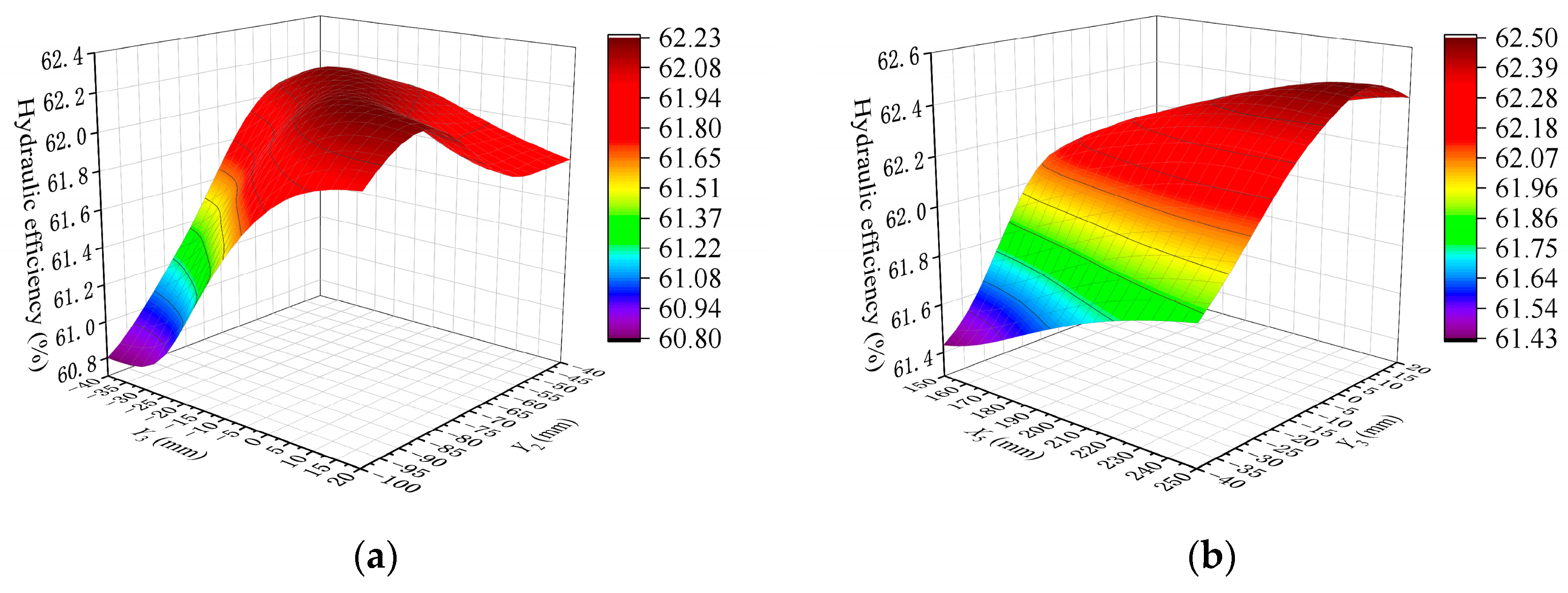
3.3.4. Search for Optimal Parameters

According to the results of the analysis, the draft tube shape optimization should be a nonlinear optimization. The SQPA can expand the objective function in a Taylor series, and this method has the characteristics of a stable solution process and high computational convergence efficiency when dealing with nonlinear optimization [31]. Therefore, the SQPA is used to find the optimal parameters. After several iterations of solving, the preliminary optimization results were obtained. Based on the correlation analysis results between different design variables and the optimization parameters, the design variables obtained from the preliminary optimization are rounded, and the results of numerical simulation after rounded are shown in

Table 5. Optimization results of draft tube shape.

	Before Optimization	After Optimization	Round Number
X2	/	69.5267	69.52
Y2	/	−75.8488	−75.84
X3	/	113.428	113.42
Y3	/	8.3927	8.4
X5	/	239.1079	239.11
Water head (m)	27.72	26.91	26.93
Hydraulic efficiency (%)	61.01	62.58	62.76

.

As can be seen from Table 5, the hydraulic efficiency of the turbine after rounding is 62.76% and the water head is 26.93 m, which indicates a significant improvement over that before optimization. In addition, the hydraulic efficiency of 62.76% is higher than all random sample points. Therefore, it can be determined that this design parameter is the optimum.

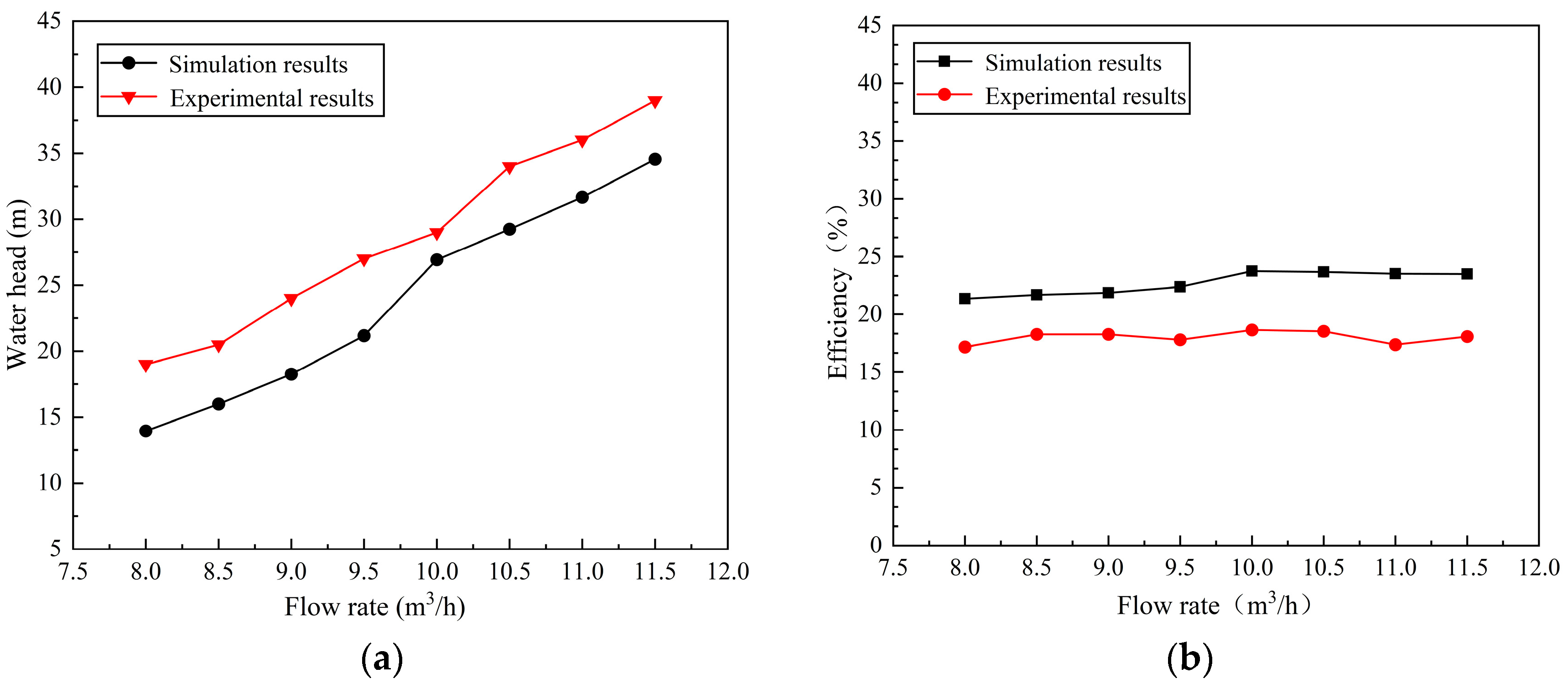
3.4. Numerical Simulation Validations

Using the lab tests to verify the accuracy of the numerical simulations for the shape-optimized draft tube. Therefore, a prototype of the turbine was manufactured to obtain the actual turbine performance of the optimized. Figure 13 shows the prototype of micro-Francis turbine after optimization. The numerical simulation outcomes and the lab test results were compared at several turbine working conditions. To perform a reasonable comparison between the results of the numerical simulation and lab tests, water head and efficiency diagrams are depicted in Figure 14 for the optimized micro-Francis turbine. It should be noted that mechanical losses, leakage losses, and generator conversion losses have been considered in the presented simulation results.

From Figure 14, it can be found that the simulated results of the water head and efficiency are consistent with the trend of the lab test results, and the best efficiency points are found at the design condition. However, the error of results between the lab test and simulation cannot be ignored. The reasons for the errors can be considered from the following three aspects:

• The numerical model of the turbine is a simplified model, which makes the hydraulic losses occurring inside the turbine not accurately predicted;
• The mechanical losses and leakage losses assessment methods used in this study were originally applied to pumps, which makes the loss assessment results inaccurate;
• There are inevitably errors in the manufacture of the prototype, instrumentation measurement errors, etc., which will have an impact on the lab test results of turbine performance.

In summary, although there are errors in the lab tests and simulation results, these errors are reasonable and acceptable. Therefore, the numerical approach chosen in this study is reliable. Additionally, the proposed micro-Francis turbine produces a power of 147 W with an efficiency of over 29% under the design conditions, which shows a considerable improvement compared to the initial prototype.

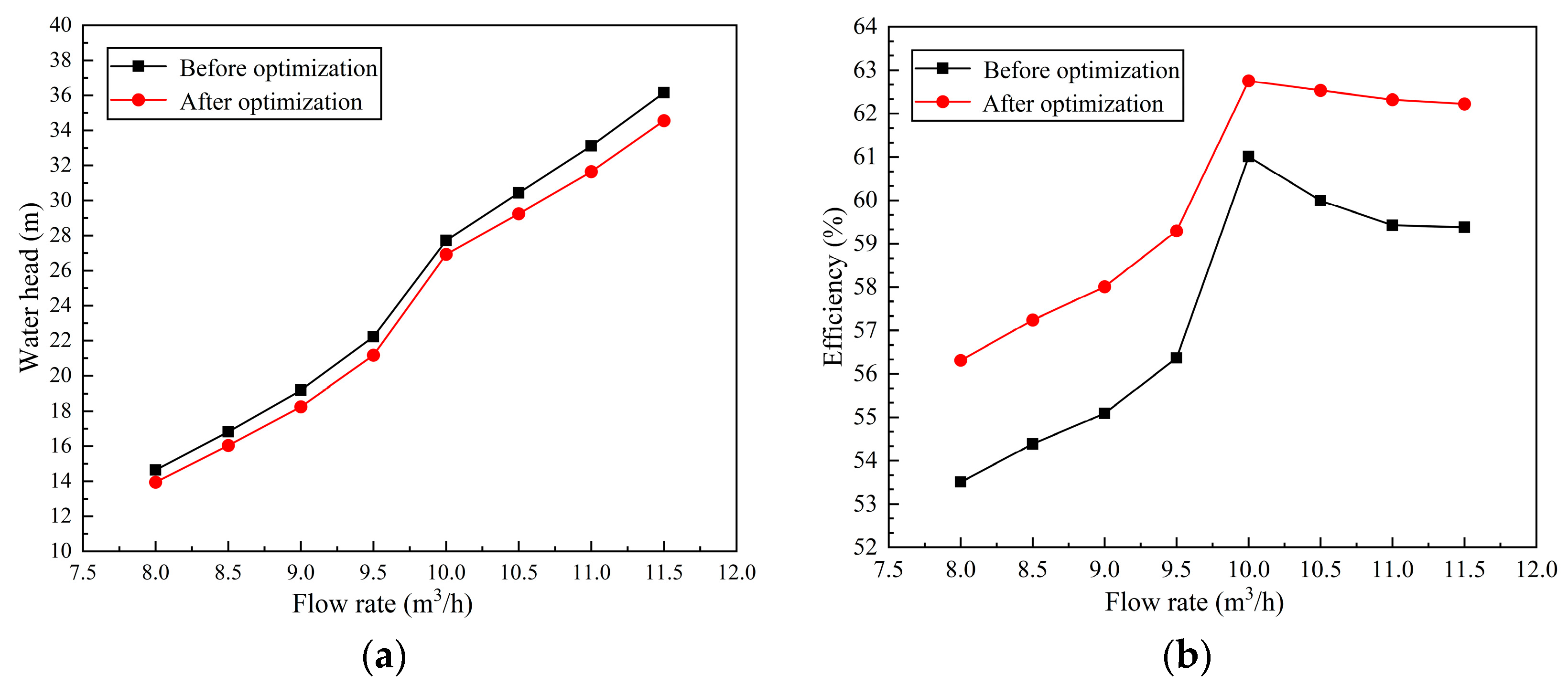
3.5. Analysis of Optimization Results

To further analyze the effect of draft tube shape optimization, the performance of the optimized turbine at non-design conditions was simulated. Figure 15 shows the simulated results of turbine performance before and after draft tube optimization at non-design conditions.

As shown in Figure 15a, the water head is significantly lower after optimization than before for the tested flow range. Although the draft tube shape optimization is carried out at the design condition, it can be seen from the results that the reduction in water head is relatively greater at the non-design condition. From Figure 15b, it can be found that the draft tube shape optimization results in a significant increase in hydraulic efficiency of the turbine in the test flow range. Corresponding to the change in water head, the increase in the hydraulic efficiency at non-design flow is relatively larger. Compared with the design condition, the flow rate at the outlet of the runner is more turbulent at the non-design condition, so an appropriate draft tube shape can play a positive effect.

Figure 16 compares the shape of the draft tube before and after optimization. It can be seen that the cross-sectional radius is equal of the draft tube after optimization. It can be predicted that the flow velocity in the draft tube and its downstream components are lower than before optimization. Therefore, the hydraulic losses such as friction and shock caused by high flow velocity will be reduced. For the location where the maximum curvature occurs, this location is closer to the draft tube inlet after optimization than before. As a result, there is a gentler transition area before the flow enters the downstream component from the location of maximum curvature in the draft tube, which results in a more stable flow at the draft tube outlet.

Figure 17 shows the velocity distribution in the draft tube outlet area before and after optimization at different flow rates. From Figure 17, it can be found that the velocity in the outlet area of the draft tube after optimization is significantly lower than that before optimization, and the high velocity area in the draft tube before and after optimization is shifted from the outside to the center area. Hence, the velocity distribution at the outlet area of the draft tube after optimization is more uniform. Additionally, before optimization, the flow lines at the draft tube outlet were mainly distributed in a spiral pattern. This anomalous flow inside the draft tube was caused by the large tangential velocity component of the water at the outlet of the runner, which led to hydraulic losses in the draft tube and downstream components. Compared to before optimization, there are still some distorted flow lines at the outlet after optimization, but the main flow is relatively stable. And consequently, the hydraulic efficiency of the turbine is significantly improved, ultimately giving rise to an increase in the turbine performance.

Based on the above analysis, the optimized model presents a notable enhancement in the hydraulic efficiency of the turbine. This efficiency improvement in the system holds the potential to greatly enhance the overall energy efficiency of the water supply system, consequently reducing the operational costs of the water supply pipeline. Additionally, the optimized draft tube facilitates a more stable water flow, effectively reducing the maintenance expenses associated with the water supply system.

4. Conclusions

In this study, a new type of micro-Francia turbine was developed for energy recovery in the WSS of high-rise buildings. The CFD simulations and lab tests were adopted to investigate the effects of the draft tube shape on the hydraulic efficiency, output power, and water head of the turbine. As inferred from the present study, the following conclusions can be obtained:

• For this micro-Francis turbine, the different radius distribution of the draft tube sections did not have a significant effect on the output power. Considering fewer input variables can lead to more accurate prediction models, the equal radius draft tube was adopted to reduce the input variables.
• A correlation analysis between design variables and optimization objectives was performed using the Pearson correlation coefficient. The results showed that the correlation coefficients r between different design variables and the optimization objective are small, which indicates that the design variables are nonlinearly correlated with the optimization objective.
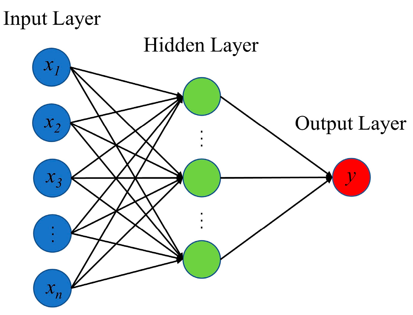
• The model errors of the standard response surface functions, radial basis function and Kriging function are compared under the same date sets, and the results showed that the R² of the radial basis function is the highest among the three, and the RMSE and MRE are both the smallest. It was verified that RBFNN has higher accuracy than other models in nonlinear approximation.
• Compared with the initial prototype, the optimized micro-Francis turbine shows a considerable improvement. The lab tests showed that the proposed turbine produces a power of 147 W with an efficiency over 29% under the design conditions.

At present, this study only discusses the external characteristics of the optimized shape of the draft tube. Therefore, subsequent studies can also investigate the effect of the change in draft tube shape on the internal characteristics of the micro-Francis turbine.

References

1. Lotfabadi, P. High-rise buildings and environmental factors. Renew. Sustain. Energy Rev. 2014, 38, 285–295. [Google Scholar] [CrossRef]
2. Park, J.H.; Chung, M.H.; Park, J.C. Development of a small wind power system with an integrated exhaust air duct in high-rise residential buildings. Energy Build. 2016, 122, 202–210. [Google Scholar] [CrossRef]
3. Wong, L.T.; Mui, K.W.; Zhou, Y. Energy efficiency evaluation for the water supply systems in tall buildings. Build. Serv. Eng. Res. Technol. 2017, 38, 400–407. [Google Scholar] [CrossRef]
4. Cheung, C.T.; Mui, K.W.; Wong, L.T. Energy efficiency of elevated water supply tanks for high-rise buildings. Appl. Energy 2013, 103, 685–691. [Google Scholar] [CrossRef]
5. Zhu, Y. Forms and problems of secondary water supply in high-rise buildings and suggestions. City Inf. 2022, 13, 232–234. [Google Scholar]
6. Du, J.; Yang, H.; Shen, Z.; Chen, J. Micro hydro power generation from water supply system in high rise buildings using pump as turbines. Energy 2017, 137, 431–440. [Google Scholar] [CrossRef]
7. Gupta, A.; Bokde, N.; Kulat, K.; Yaseen, Z.M. Nodal Matrix Analysis for Optimal PRV Localization in a Water Distribution System. Energies 2020, 13, 1878. [Google Scholar] [CrossRef]
8. Kougias, I.; Aggidis, G.; Avellan, F.; Deniz, S.; Lundin, U.; Moro, A.; Muntean, S.; Novara, D.; Pérez-Díaz, J.I.; Quaranta, E.; et al. Analysis of emerging technologies in the hydropower sector. Renew. Sustain. Energy Rev. 2019, 113, 109257. [Google Scholar] [CrossRef]
9. Okot, D.K. Review of small hydropower technology. Renew. Sustain. Energy Rev. 2013, 26, 515–520. [Google Scholar] [CrossRef]
10. Liu, X.; Luo, Y.; Karney, B.W.; Wang, W. A selected literature review of efficiency improvements in hydraulic turbines. Renew. Sustain. Energy Rev. 2015, 51, 18–28. [Google Scholar] [CrossRef]
11. Sari, M.A.; Badruzzaman, M.; Cherchi, C.; Swindle, M.; Ajami, N.; Jacangelo, J.G. Recent innovations and trends in in-conduit hydropower technologies and their applications in water distribution systems. J. Environ. Manag. 2018, 228, 416–428. [Google Scholar] [CrossRef] [PubMed]
12. Xiong, C.; Yu, B.; Li, W. Design and Performance Forecasting of Micro-channeis Turbine Based on Numerical Test. China Rural Water Hydropower 2009, 2, 130–132. [Google Scholar]
13. Guo, H.; Wang, H.; Zheng, Y.; Shi, J.; Kan, K. Optimal design of micro-pipe turbine based on orthogonal test method. J. Drain. Irrig. Mach. Eng. (JDIME) 2022, 40, 928–935. (In Chinese) [Google Scholar]
14. Graciano-Uribe, J.; Sierra, J.; Torres-Lopez, E. Instabilities and influence of geometric parameters on the efficiency of a pump operated as a turbine for micro hydro power generation: A review. J. Sustain. Dev. Energy Water Environ. Syst. 2021, 9, 1–23. [Google Scholar] [CrossRef]
15. Arispe, T.M.; de Oliveira, W.; Ramirez, R.G. Francis turbine draft tube para-meterization and analysis of performance characteristics using CFD techniques. Renew. Energy 2018, 127, 114–124. [Google Scholar] [CrossRef]
16. Chen, Z.; Baek, S.H.; Cho, H.; Choi, Y.D. Optimal design of J-groove shape on the suppression of unsteady flow in the Francis turbine draft tube. J. Mech. Sci. Technol. 2019, 33, 2211–2218. [Google Scholar] [CrossRef]
17. Zhou, X.; Wu, H.; Cheng, L.; Huang, Q.; Shi, C. A new draft tube shape optimisation methodology of introducing inclined conical diffuser in hydraulic turbine. Energy 2023, 265, 126347. [Google Scholar] [CrossRef]
18. Dai, C.; Che, H.; Leung, M.F. A neurodynamic optimization approach for l 1 minimization with application to compressed image reconstruction. Int. J. Artif. Intell. Tools 2021, 30, 2140007. [Google Scholar] [CrossRef]
19. Hasanzadeh, N.; Payambarpour, S.A.; Najafi, A.F.; Magagnato, F. Investigation of in-pipe drag-based turbine for distributed hydropower harvesting: Modeling and optimization. J. Clean. Prod. 2021, 298, 126710. [Google Scholar] [CrossRef]
20. Mengistu, T.; Ghaly, W. Aerodynamic optimization of turbomachinery blades using evolutionary methods and ANN-based surrogate models. Optim. Eng. 2008, 9, 239–255. [Google Scholar] [CrossRef]
21. Du, J.; Ge, Z.; Wu, H.; Shi, X.; Yuan, F.; Yu, W.; Wang, D.; Yang, X. Study on the effects of runner geometric parameters on the performance of micro Francis turbines used in water supply system of high-rise buildings. Energy 2022, 256, 124616. [Google Scholar] [CrossRef]
22. Zhang, H.; Long, C.; Hu, S.-Y.; Liao, K.; Gao, Y.W. Topology verification method of a distribution network based on hierarchical clustering and the Pearson correlation coefficient. Power Syst. Prot. Control 2021, 49, 88–96. [Google Scholar]
23. Luo, F.; Zhang, X.; Yang, X.; Yao, Z.; Zhu, L.; Qian, M. Load Analysis and Prediction of Integrated Energy Distribution System Based on Deep Learning. High Volt. Eng. 2021, 47, 23–32. [Google Scholar]
24. Wu, R.; Yao, Y.; Li, G. Multi-objective optimization of high-speed locomotive lateral dynamics performance based on RBFNN surrogate model. J. Cent. South Univ. (Sci. Technol.) 2023, 54, 1644–1652. [Google Scholar]
25. Tong, S.; He, S.; Tong, Z.; Fan, H.; Li, Y.; Tan, D.; Zhong, Y. Lightweight Design Method Based on Combined Approximation Model. China Mech. Eng. 2020, 31, 337–1343. [Google Scholar] [CrossRef]
26. Wang, X.; Li, Z.; Liu, D. Optimization of Glass Drilling Support Structure Based on Response Surface Method. Modul. Mach. Tool Autom. Manuf. Tech. 2021, 2, 131–135. [Google Scholar] [CrossRef]
27. Shrestha, U.; Choi, Y.-D. A CFD-Based Shape Design Optimization Process of Fixed Flow Passages in a Francis Hydro Turbine. Processes 2020, 8, 1392. [Google Scholar] [CrossRef]
28. Du, J.; Shen, Z.; Guo, X. Development of an inline vertical cross-flow turbine for hydropower harvesting in urban water supply pipes. Renew. Energy 2018, 127, 386–397. [Google Scholar]
29. Du, J.; Yang, H.; Shen, Z. Study on the impact of blades wrap angle on the performance of pumps as turbines used in water supply system of high-rise buildings. Int. J. Low-Carbon Technol. 2018, 13, 102–108. [Google Scholar] [CrossRef]
30. Kim, S.-J.; Choi, Y.-S.; Cho, Y.; Choi, J.-W.; Kim, J.-H. Effect of blade thickness on the hydraulic performance of a Francis hydro turbine model. Renew. Energy 2019, 134, 807–817. [Google Scholar] [CrossRef]
31. Long, L.; Xue, P.; Liu, J.; Wang, K.; Tan, Z. Optimization of Lattice Sandwich Structure With Sequential Quadratic Programming Algorithm. J. Beijing Univ. Technol. 2016, 42, 45–49. [Google Scholar]
Figure 1. Research flow chart.
Processes 12 01128 g001
Figure 2. Flow channel diagram of Francis turbine.
Processes 12 01128 g002
Figure 3. Sketch of draft tube shape definition.
Processes 12 01128 g003
Figure 4. Draft tube shape control. (a) Central line shape control. (b) Boundary line shape control.
Processes 12 01128 g004
Figure 5. Schematic diagram of RBFNN.
Processes 12 01128 g005
Figure 6. Meshing result of simulated model.
Processes 12 01128 g006
Figure 7. Schematic diagram of hydraulic test rig.
Processes 12 01128 g007
Figure 8. Hydraulic test rig for Francis turbine test.
Processes 12 01128 g008
Figure 9. 3D modeling of draft tube of different projects.
Processes 12 01128 g009
Figure 10. Simulation results of different project.
Processes 12 01128 g010
Figure 11. Calculation results of Pearson correlation coefficient.
Processes 12 01128 g011
Figure 12. The 3D surface maps of RBFNN. (a) Y2, Y3 and hydraulic efficiency. (b) Y3, X5 and hydraulic efficiency.
Processes 12 01128 g012
Figure 13. Prototype of micro-Francis turbine after system optimization.
Processes 12 01128 g013
Figure 14. Numerical and lab tests results comparison of water head and efficiency. (a) Comparison of water head. (b) Comparison of efficiency.
Processes 12 01128 g014
Figure 15. Simulation results of draft tube optimization before and after. (a) Water head. (b) Efficiency.
Processes 12 01128 g015
Figure 16. Shape of draft tube before and after optimization.
Processes 12 01128 g016
Figure 17. Velocity distribution in draft tube outlet area before and after optimization.
Processes 12 01128 g017