Abstract
The classification of microseismic signals represents a fundamental preprocessing step in microseismic monitoring and early warning. A microseismic signal source rock classification method based on a convolutional neural network is proposed. First, the characteristic parameters of the microseismic signals are extracted, and a convolutional neural network is constructed for the analysis of these parameters; then, the mapping relationship model between the characteristic parameters of the microseismic signals and the rock class is established. The feasibility of the proposed method in differentiating acoustic emission signals under different load conditions is verified by using acoustic emission data from laboratory uniaxial compression tests, Brazilian splitting tests, and shear tests. In the three distinct laboratory experiments, the proposed method achieved a source rock classification accuracy of greater than 90% for acoustic emission signals. The proposed and verified method provides a new basis for the preprocessing of microseismic signals.
1. Introduction
In recent years, the increasing demand for mineral resources has led mining companies to gradually expand their operations to deeper underground levels. However, underground excavation activities disrupt the natural stress equilibrium of the surrounding rock mass. The excavation process generates voids that release stored strain energy within the rock mass, resulting in rock mass failure and dynamic events such as ground pressure bursts and sudden inflows of water, contributing to mining-induced dynamic disasters [1,2]. Mining-induced dynamic disasters possess significant destructive power and high levels of hazard. They exhibit characteristics such as abrupt occurrence, complex mechanisms, and numerous influencing factors. Currently, research on mining-induced dynamic disasters has become a key and challenging aspect of underground mining safety efforts [3,4].
Microseismic monitoring is currently the most widely employed method for monitoring mining-induced dynamic disasters. It involves the use of acoustic-electric sensors to monitor the generation of elastic waves during the rock mass failure process, thereby obtaining spatiotemporal strength information related to microseismic events and facilitating the prediction of mining-induced dynamic disasters [5,6,7,8]. Before predicting mining-induced dynamic disasters, a series of preprocessing steps are required for microseismic signals: microseismic signal classification [9,10,11,12,13], microseismic signal denoising [14,15], initial arrival time picking [16,17], and seismic source localization [18,19,20]. Microseismic signal classification represents the first step in the preprocessing of microseismic signals and is a crucial component to ensure the effectiveness of subsequent procedures. The microseismic signals acquired via microseismic monitoring systems can be categorized into genuine microseismic signals and non-microseismic signals. The amplitude, frequency, and other characteristics of genuine microseismic signals are often used to reveal the state of rock failure. Some scholars [21,22,23] have conducted laboratory acoustic emission experiments to demonstrate the significant differences in the evolution patterns of microseismic characteristic parameters during the failure process of various rock types. Song [24] investigated the evolution of absolute acoustic emission energy and cumulative acoustic emission energy during the uniaxial compression failure process of granite under different loading rates. Li [25] investigated the mechanical behaviors and the variations in acoustic emission characteristic parameters, including event counts, cumulative counts, and energy, during the uniaxial compression failure process of sandstone. Xu [26] studied the variations in acoustic emission event counts and duration during the fracture failure process of limestone specimens. Wang [27] investigated the frequency-domain variations in acoustic emission energy during the failure process of limestone under Brazilian splitting loading conditions. Guo [28] characterized the failure process of coal under Brazilian splitting loading conditions using acoustic emission parameters such as energy, frequency counts, and amplitude, and compared them jointly with mechanical damage laws. Ban [29] investigated the variations in acoustic emission energy parameters during the failure process of rock-like materials under shear loading conditions. Luo [30] studied the patterns of cumulative acoustic emission counts and amplitudes during the failure process of red sandstone under various shear angle conditions. Li [31] conducted a comparative analysis of the differences in acoustic emission count variations during the failure process of red sandstone under three different loading conditions: uniaxial compression, Brazilian splitting, and shear. Li [32] compared the differences in acoustic emission B-values and peak frequency variations during the failure process of rocks from different geological formations, such as granite, sandstone, and marble, within the same region under Brazilian splitting loading conditions. These studies show that the characteristics of microseismic signals generated by different rocks under stress vary significantly, and accurately identifying the types of rocks that generate microseismic signals can help to more precisely judge the stress state and potential failure location inside the rock mass, thus improving the accuracy of early warning systems. Vallejos and McKinnon [33] introduced an algorithm for classifying microseismic events and explosions based on multiple source parameters and logistic neural networks. Meier [34] combined a generative adversarial network with a random forest classifier to discriminate between seismic signals and noise. Provost [35] used random forest surveillance to build a classifier that automatically identifies microseismic signals, seismic signals, and noise signals. Wilkins [36] used a convolutional neural network to accurately identify and select a large number of microseismic signals collected via the microseismic monitoring system in coal mine. Ma [37] introduced a Bayesian discriminative method that is based on source parameters and waveform characteristics, and they validated this method using microseismic data from a mine. Shang [38] trained an artificial neural network model using 22 parameters derived from principal component analysis as input features, which resulted in an enhanced accuracy in discriminating between genuine microseismic signals and explosion signals. This model was subsequently applied to the Junde underground mine, yielding a high level of accuracy. Tang [39] introduced deep spatial and channel attention modules and established an improved network architecture suitable for complex signal recognition and classification. The research findings of these scholars have achieved the identification of genuine microseismic signals from non-microseismic ones. On the other hand, Chien [40] built a convolutional self-coding network to identify real microseismic signals, classifying them according to the depth of the formation at which they were generated. Mousavi [41] studied the signal characteristics of deep and shallow microearthquakes and clustered them based on these characteristics using machine learning techniques. Few researchers have delved further into distinguishing the source rock types for microseismic signals. However, mines exist within complex geological environments where different rock strata are composed of various types of rocks. The rock failure detected using the microseismic system comprises a mixture of different types of microseismic signals. This complexity can introduce a certain degree of error when utilizing microseismic signals for mining-induced dynamic disaster prediction and assessment. Therefore, after distinguishing real microseismic signals from non-microseismic signals, it is necessary to further distinguish the types of rocks that generate microseismic signals.
In this study, we designed and explored a CNN-based classification model to identify source rock types generating microseismic signals using feature parameters from raw microseismic signals. The classification model associates the extracted feature parameters from raw microseismic signals with the corresponding rock types. Using the trained classification model, complex microseismic signals can be identified, providing the corresponding source rock types. Additionally, acoustic emission signals from laboratory uniaxial compression tests, shear tests, and Brazilian splitting tests were used to simulate the microseismic signals of actual rock failures in mines.
The overall structure of this article consists of four sections, including this introductory section. Section 2 presents the laboratory tests for obtaining microseismic signals, the design of a neural network for microseismic signal type recognition and the model training details. Section 3 describes the training process and test results of the new method under three different experimental conditions, while Section 4 provides an analysis of the experimental results, potential application value, shortcomings of the research, and future directions.
2. Materials and Methods
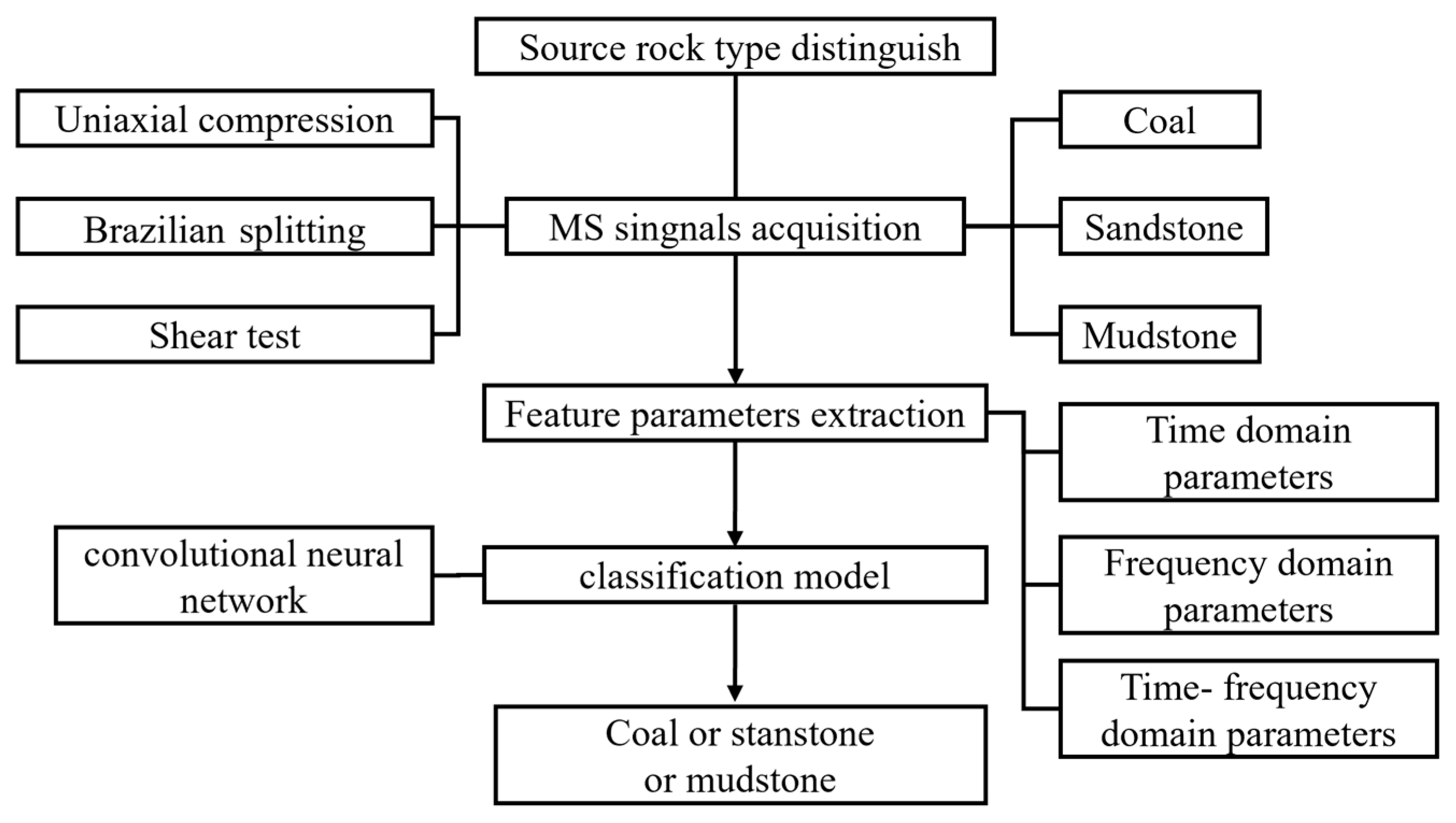
The proposed method for classifying the source rock types of microseismic signals (MS) integrates the Fourier transform with convolutional neural networks. The workflow of this method is illustrated in Figure 1 and consists of three key steps: (1) Establishing a dataset of microseismic signal features and a basic convolutional neural network framework; (2) training a model to map the relationship between microseismic signal features and source rock type labels; (3) application to new microseismic signals.

Figure 1.
Workflow source rock type identification for real microseismic signals.
2.1. Microseismic Signals Acquisition
In this section, microseismic signals are simulated by utilizing acoustic emission (AE) signals obtained from laboratory experiments. Following the standard test method of the International Society of Rock Mechanics [42], laboratory acoustic emission (AE) experiments involving uniaxial compression, Brazilian splitting, and shear tests were conducted on various rock specimens to simulate the distinct failure processes of deep-seated rocks.
2.1.1. Compressive Loading Test
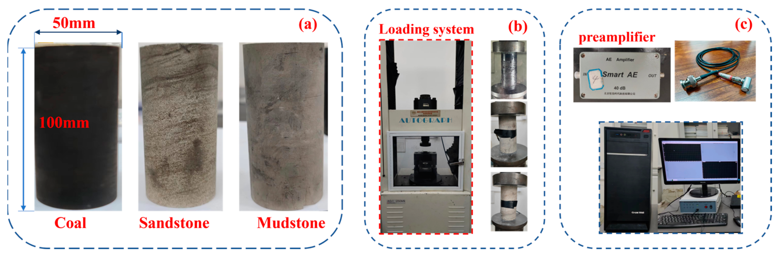
The process of simulating microseismic signals generated by rock failure under compression was conducted through uniaxial compression acoustic emission signal experiments, as depicted in Figure 2. The rock specimens used in this study, as shown in Figure 2a, were collected from the same coal seam, overlying aquifer, and aquitard within a single mine and working face. These specimens represented coal, sandstone, and mudstone, respectively (Zhalainuoer Coal Industry Co., Ltd., Hulunbuir, China). The rock specimens were cylindrical in shape with a diameter of 50 mm and a height of 100 mm. The mechanical loading system employed is depicted in Figure 2b and consisted of a Shimadzu AG-250KN (Shimadzu Co., Ltd., Kyoto Prefecture, Japan) mechanical testing machine. Displacement-controlled loading was used with a loading rate set at 0.05 mm/s. The acoustic emission monitoring setup, depicted in Figure 2c, utilized a Soft-Ice DS2 (Beijing Soft Island Times Technology Co., Ltd., Beijing, China) acoustic emission monitoring instrument with a sampling rate of 3 MHz, a threshold of 20 mV, a pre-amplifier gain of 40 dB, and RS-54A sensors.
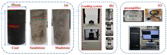
Figure 2.
Uniaxial compression acoustic emission signal experiments. (a) Test sample, (b) mechanical loading system, (c) acoustic emission monitoring system.
The specific test process is as follows: Firstly, the acoustic emission sensor is attached to the surface of the sample, with the center of the cylindrical side surface used for the uniaxial compression test, and the center of the circular bottom surface used for the Brazilian splitting and shear test. A coupler is applied between the specimen and the sensor. The sample is then placed vertically in the center of the lower seat of the press, and the position of the upper indenter is adjusted to be close to the sample. Finally, the pressure loading system and the acoustic emission monitoring system are started simultaneously until the sample is damaged.
2.1.2. Shear Loading Test
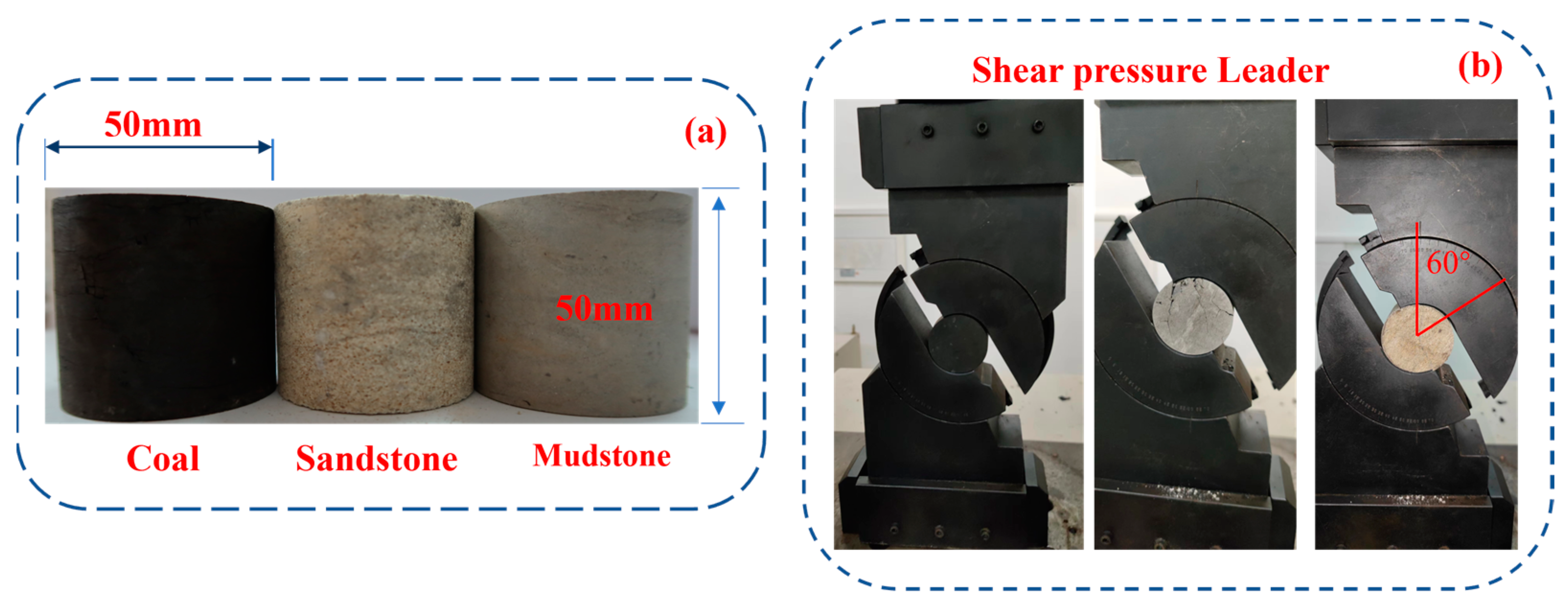
In this section, laboratory shear tests were conducted to simulate the scenario of rock mass failure under shear stress. The rock specimen types and sources utilized in Figure 3a were identical to those employed in the uniaxial compression test, except for a variation in specimen dimensions, with a diameter and height of 50 mm each. Similarly, the recognition types and parameters of the loading and monitoring systems used remained consistent with the previous experiment, except for the loading pressure head, which was replaced with a shear pressure head set at a shear angle of 60°, as illustrated in Figure 3b.
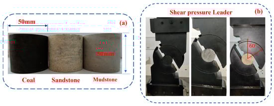
Figure 3.
Shear failure acoustic emission signal experiments. (a) Test sample, (b) mechanical loading system.
2.1.3. Indirect Tensile Loading Test
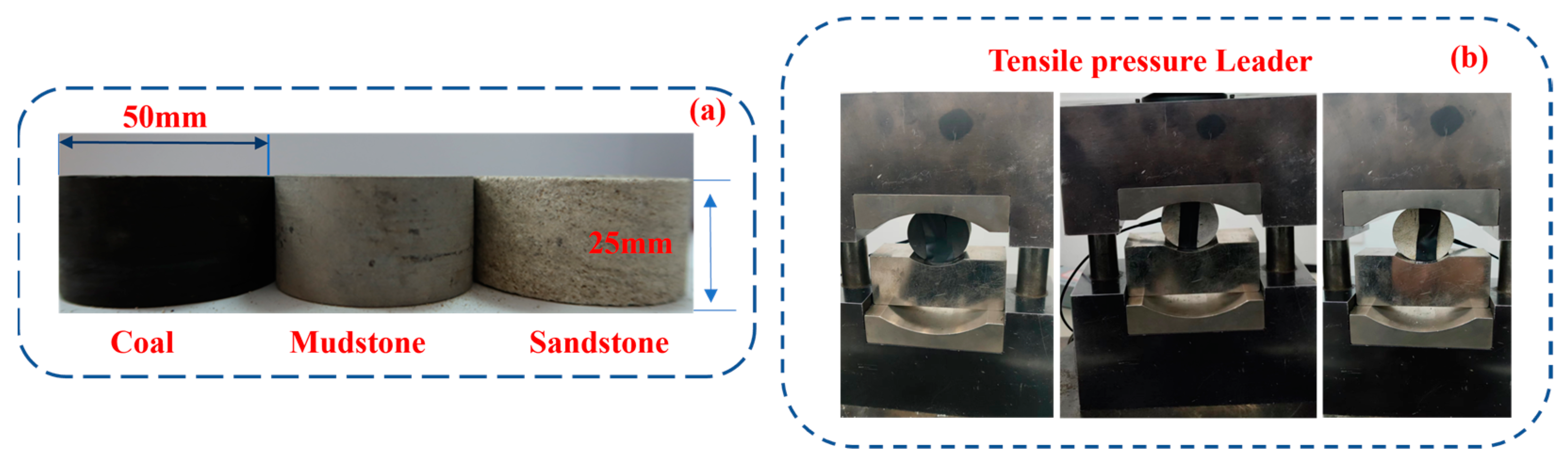
The fracture of rocks under tensile loading is a common failure mode in deep-seated rock formations. Therefore, in this section, the proposed method is validated for discriminating rock types using acoustic emission signals generated during laboratory Brazilian splitting tests, serving as an indicator of its effectiveness in distinguishing rock types based on microseismic signals produced during tensile failure. During the laboratory Brazilian splitting test, the types and parameter settings of the mechanical loading machine and acoustic emission monitoring device were the same as in the previous two tests. It should be noted that, in this test, the specimen used was a flat cylinder with a height of 25 mm and a diameter of 50 mm, as shown in Figure 4a. The loading head used was replaced with a tensile stress loader, as shown in Figure 4b.
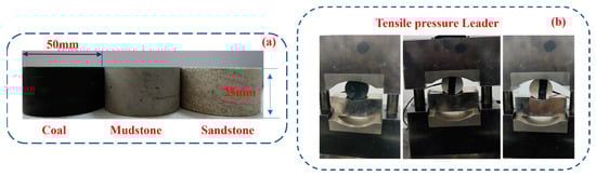
Figure 4.
Tensile failure acoustic emission signal experiments. (a) Test sample, (b) mechanical loading system.
2.1.4. Feature Parameters Extraction
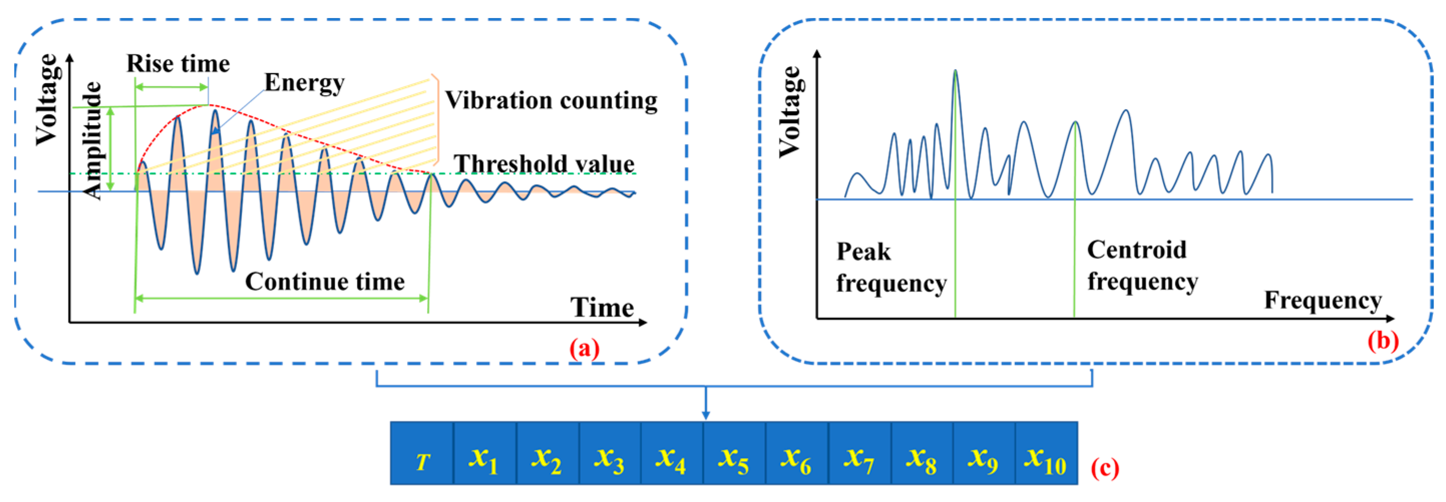
After collecting microseismic signals, 10 microseismic shape feature parameters need to be extracted from them to serve as input parameters for the machine learning model, as shown in Figure 5a,b. As illustrated in Figure 5c, x1 to x8 represent time-domain characteristics: amplitude, continuous time, rise time, rise count, vibration count, energy, effective voltage, and average level. x9 and x10 represent frequency-domain parameters obtained through Fourier transformation: centroid frequency and peak frequency, respectively. These parameters are then flattened into a one-dimensional feature matrix, which serve as the input features for the model. The labels are assigned based on the lithology of the rock formations. It is important to note that the microseismic signals in the dataset should originate from the same microseismic monitoring area to ensure data consistency.
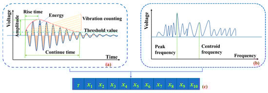
Figure 5.
Overview of common microseismic signal parameters used for rock type identifying. (a) Time domain characteristic parameter; (b) Frequncy domain characteristic parameter; (c) One-dimensional eigenparameter matrix; x1~x10 is the value of the feature parameter, T is the rock type of the damage source corresponding to the microseismic signal.
2.2. Type Identification Convolutional Neural Network (T_Net)
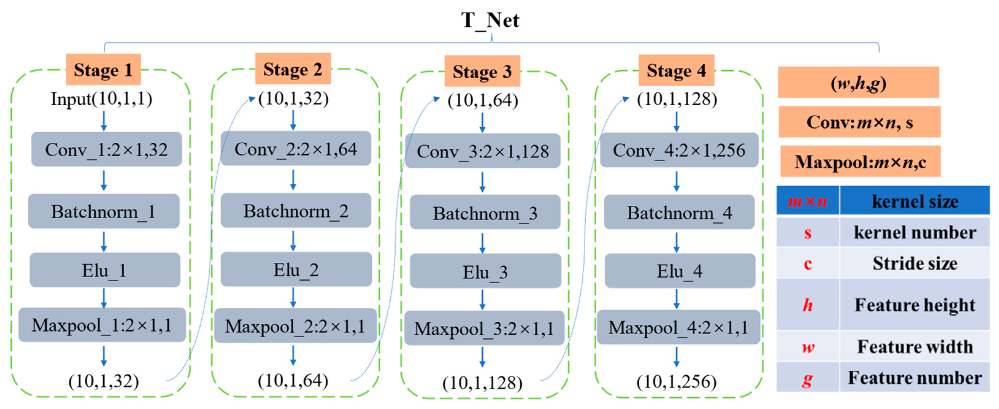
Figure 6 illustrates the T_Net, which is constructed based on microseismic signal feature parameters and comprises a total of 16 layers organized into 4 convolutional modules. Each convolutional module consists of a convolutional computation layer, a batch normalization layer, an activation function layer, and a max-pooling layer.
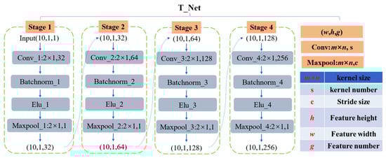
Figure 6.
Network structure and parameter composition of T_Net.
In the convolutional layers of the 4 convolutional modules, the convolutional kernel size is consistently set to (2 × 1) with a stride of 1. The number of generated convolutions for each module is 32, 64, 128, and 256, respectively. The input feature is a 10 × 1 feature matrix, and after the convolutional computations, it yields an output matrix comprising 256 microseismic signal feature parameters. The convolution operation can be expressed as the following Equation (1) [43]:
where, g, p represent the index of the output feature map, and m, n represent the index of the convolution kernel.
After the convolutional layers, a batch normalization layer is inserted. This is because parameters during the training process may undergo real-time variations, which can lead to changes in the data distribution of the microseismic signal feature matrix after convolutional computations. The placement of the batch normalization layer addresses the situation where the data distribution in intermediate layers changes during training, making the process of training the network model smoother and more stable. The implementation of batch normalization can be represented using the following Equations (2)–(5):
where, xi,j represents the value of the jth characteristic parameter in the ith microseismic signal characteristic matrix. i is the number of microseismic signals in the same batch, and j is the number of microseismic signal characteristic parameters in the matrix.
where, μj represents the mean value of the class j characteristic parameters of microseismic signals.
where, represents the variance of the class j characteristic parameters of microseismic signals.
where, yi,j represents the variance of the xi,j batch normalized value, γ is the scale factor, ε is the small positive numbers used when the divisor is 0.
Considering that microseismic waveforms exhibit both positive and negative amplitude points, making them susceptible to noise interference, the Exponential Linear Unit (ELU) activation function has been chosen as the appropriate activation function within the T_Net. The ELU function helps address this issue by allowing the representation of both positive and negative values while mitigating the adverse impact of noise. The characteristics of the ELU function make it suitable for preserving the dynamic range and reducing the degradation caused by noise interference in the analysis of microseismic waveforms. The ELU function can be expressed as the following Equation (6) [44]:
where α represents a scalar that represents the slope of the negative portion.
Within the T_Net framework, the maximum pooling strategy is employed, where the maximum value within each pooling region serves as the selected pooling result. This selection criterion aids in preserving the most salient features within the downsampled feature maps.
2.3. Model Training
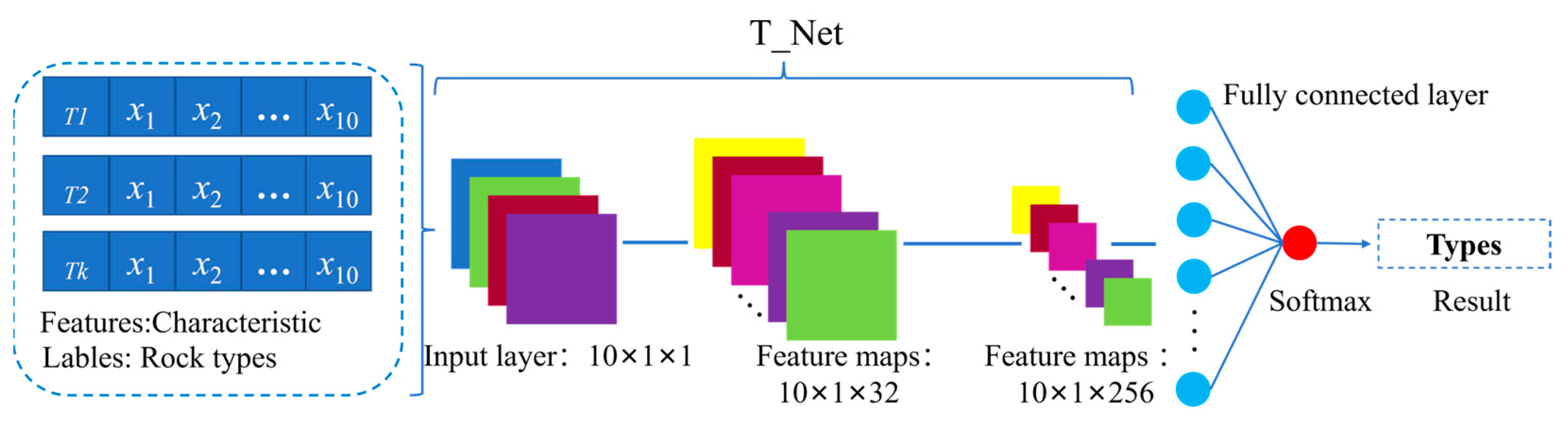
Figure 7 illustrates that during the model training process, the input layer takes the one-dimensional feature parameter matrix of microseismic signals as the model’s input, with the corresponding source rock type serving as the label. Within the training layers, the T_Net network, constructed as the foundational framework, learns the mapping relationship between the parameter matrix and the source rock type. The final output represents the most suitable source rock type for the microseismic signal.
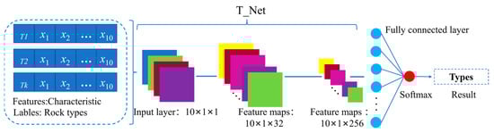
Figure 7.
Training framework and hyperparameter setting of rock class recognition model for microseismic signals.
2.3.1. Data Set
In the uniaxial compression test, a total of 7681 acoustic emission signals were collected, comprising 430 signals from sandstone, 6618 from mudstone, and 633 from coal. For the shear test, 6792 acoustic emission signals were collected, with 859 from sandstone, 846 from mudstone, and 5087 from coal. The Brazilian splitting test yielded 6935 acoustic emission signals, with 6065 from sandstone, 769 from mudstone, and 101 from coal. The dataset was divided into a 90% training set and a 10% test set. The final division results are shown in Table 1 below.

Table 1.
Data set partitioning results.
2.3.2. Hyperparameter Settings
The hyperparameters for model training include the use of the Adam optimization algorithm, a maximum of 5000 training steps, an initial learning rate of 0.001, a regularization parameter of 0.0001, and a learning rate that decreases by a factor of 0.5. The cross-entropy loss function is used to minimize prediction errors and facilitate model convergence. All experiments were conducted on a PC equipped with an NVIDIA GeForce 2080 Ti GPU and 64 GB RAM, using Matlab R2018a (Meiswalker Software (Beijing) Co., Ltd., Beijing, China) to construct the neural networks. This configuration was used for both model training and testing in all subsequent test examples.
The trained model can be employed for the source rock type classification of new microseismic signals related to the source of damage. However, it is important to note that the training data and the application data must originate from the same mine or project site. If there is a need to utilize the model in different projects, it is imperative to gather microseismic waveform data anew and conduct retraining of the model.
3. Results
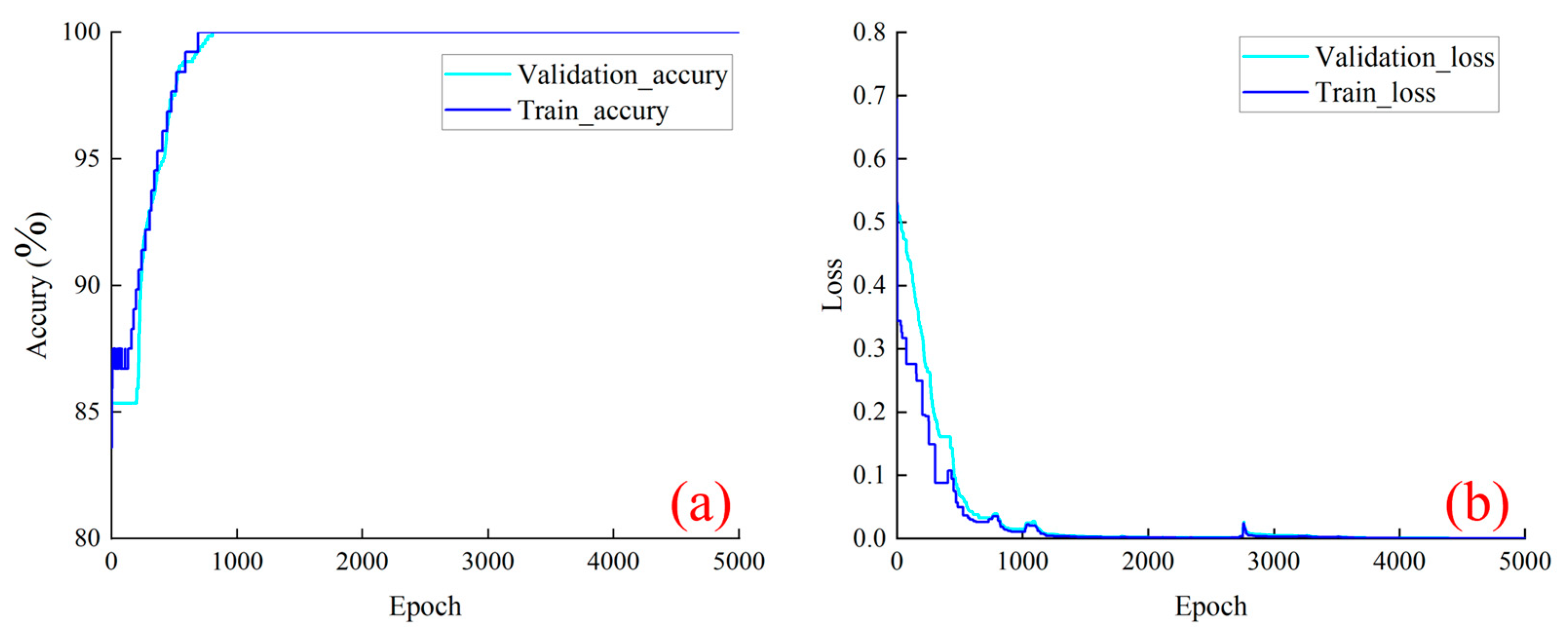
Figure 8a,b illustrate the variations in training set loss and accuracy (blue curves) and validation set variations (cyan curves) during the model training process. Throughout the entire training process, the training loss slightly outperforms the validation loss, as observed from the loss and accuracy curves. Both curves exhibit a rapid descent trend in the initial 1000 training epochs, followed by a gradual descent over the subsequent 3600 training epochs. The validation loss and accuracy stabilize after the 1000th epoch, with only a slight decrease from 0.01 to 0.003, whereas the training loss drops significantly from 1 to 0.1 during the first 1000 epochs. The training recognition accuracy sharply increases in the first 1000 iterations and subsequently stabilizes at around 99.9%. The continual decrease in both training and validation losses, coupled with the ascent in accuracy, validates that the proposed T_Net network has learned the mapping relationship between acoustic emission waveform parameters and the types of fractured rocks.
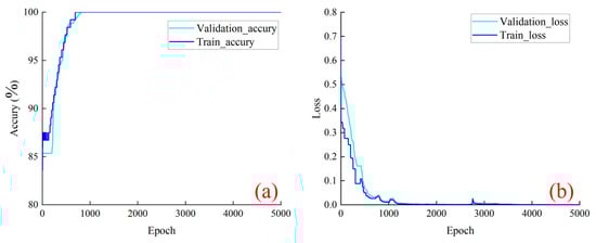
Figure 8.
The loss and accuracy variation for model training and validating under uniaxial compression failure mode. (a) Training and Validation accuracy during model training; (b) Training and Validation loss during model training.
The recognition accuracy of the test set’s acoustic emission signal identification, as depicted in Figure 9a,b, is as follows: sandstone—97.5%, mudstone—100%, and coal—98.3%. In terms of the misclassification of acoustic emission signals, signals originating from sandstone may be incorrectly classified as coal, while signals from coal–sandstone may be misclassified as sandstone. However, sandstone is not misclassified as mudstone, nor is it misclassified as both coal and mudstone. This section may be divided into subheadings and should provide a concise and precise description of the experimental results, their interpretation, as well as the experimental conclusions that can be drawn.
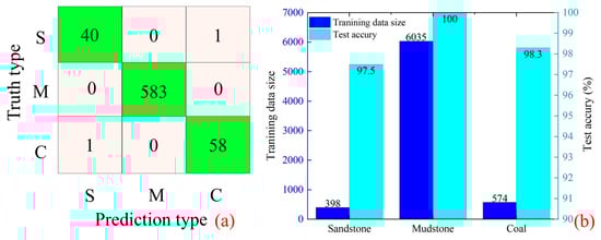
Figure 9.
Test results of the model under uniaxial compression failure mode. S stands for sandstone, M stands for mudstone, C stands for coal. (a) Test set data identification result confusion matrix; (b) Training set data and test set recognition accuracy.
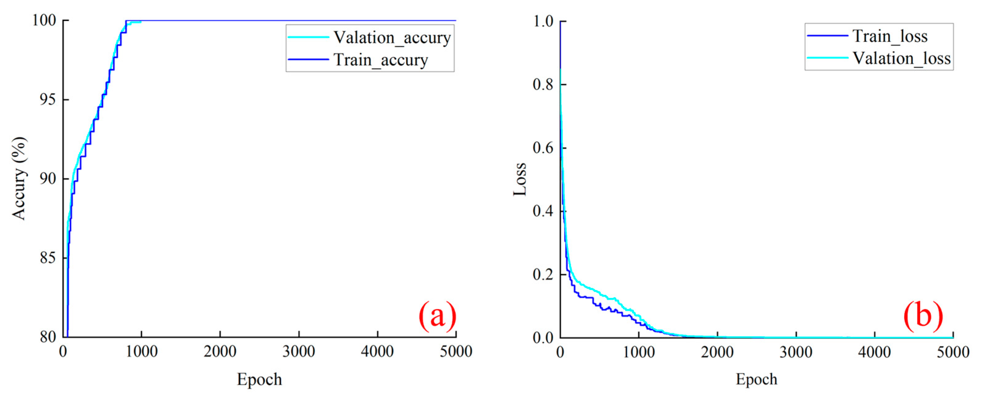
When the model is applied to the recognition of rock types based on acoustic emission signals under shear stress conditions, as depicted in Figure 10a,b, the training set loss and accuracy (blue curves) and validation set variations (cyan curves) during the model training process reveal that, by the end of the training, both curves will converge similarly to the previous experiment, approaching 0% loss and 100% accuracy. However, it is noteworthy that the loss curve experiences a sudden change near the 1500th step, which is relatively delayed compared to the uniaxial compression test.
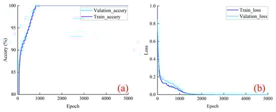
Figure 10.
The loss and accuracy variation for model training and validating under shear failure mode. (a) Training and Validation accuracy during model training; (b) Training and Validation loss during model training.
As illustrated in Figure 11a,b, the recognition accuracy of the test set’s acoustic emission signal identification is as follows: sandstone—97%, mudstone—96.9%, and coal—100%. Notably, the highest recognition accuracy shifts from mudstone to coal. Additionally, in terms of the misclassification of acoustic emission signals, the transition to coal no longer results in misidentification as sandstone or mudstone, but rather mutual misclassifications occur between sandstone and mudstone.
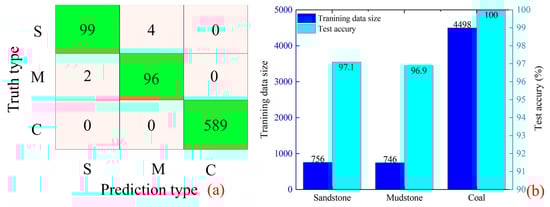
Figure 11.
Test results of the model under shear failure mode. S stands for sandstone, M stands for mudstone, C stands for coal. (a) Test set data identification result confusion matrix; (b) Training set data and test set recognition accuracy.
When the model is applied to the recognition of rock types based on acoustic emission signals under tensile stress conditions, as depicted in Figure 12a,b, the training set loss and accuracy (blue curves) and validation set variations (cyan curves) during the model training process reveal that, by the end of model training, both curves will converge similarly to the previous experiment, approaching 0% loss and 100% accuracy. However, it is noteworthy that the loss curve experiences a sudden change near the 600th step. Compared with the first two tests, the convergence rate of this model is the fastest.
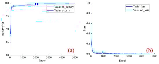
Figure 12.
The loss and accuracy variation for model training and validating under tensile failure mode. (a) Training and Validation accuracy during model training; (b) Training and Validation loss during model training.
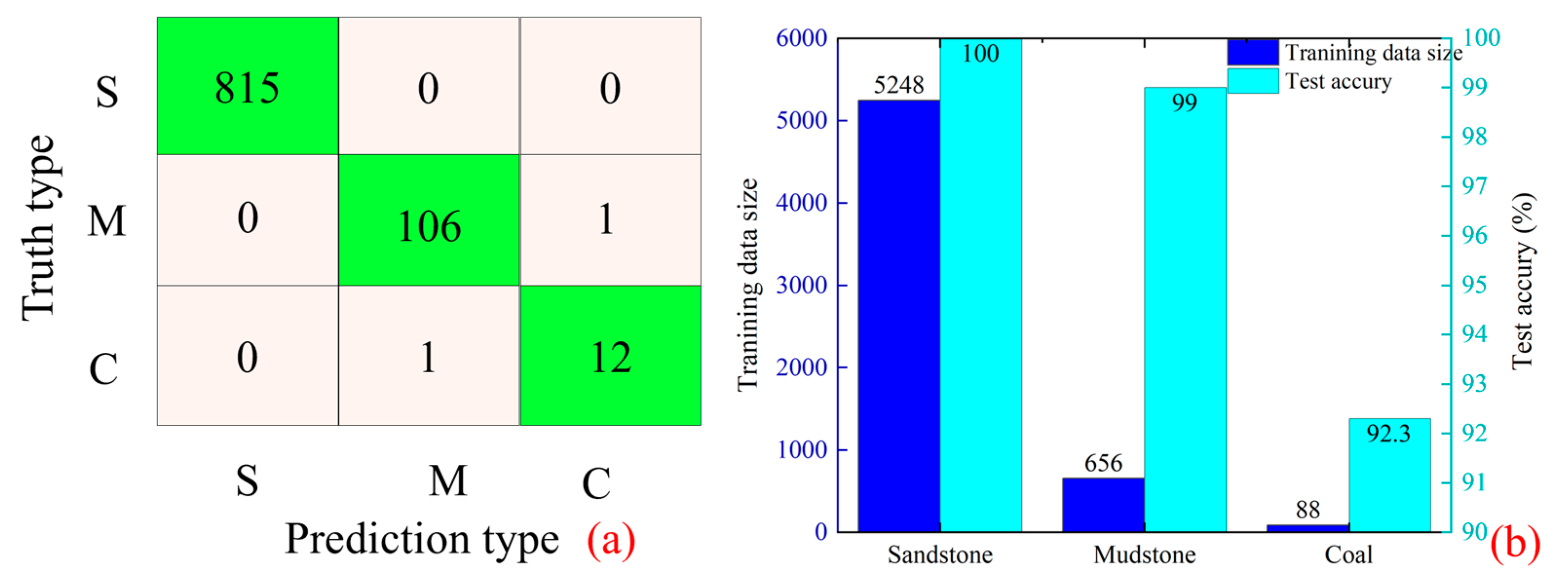
As illustrated in Figure 13a,b, the recognition accuracy of the test set’s acoustic emission signal identification is as follows: sandstone—100%, mudstone—99%, and coal—92.3%. It is worth noting that sandstone has the highest identification accuracy. Addition-ally, in terms of the misclassification of acoustic emission signals, the transition to sandstone no longer results in misidentification as coal or mudstone, but rather, mutual misclassifications occur between coal and mudstone.

Figure 13.
Test results of the model under tensile failure mode. S stands for sandstone, M stands for mudstone, C stands for coal. (a) Test set data identification result confusion matrix; (b) Training set data and test set recognition accuracy.
The proposed method achieved a source rock type classification accuracy of over 90% for acoustic emission signals in three distinct laboratory experiments, demonstrating the feasibility of source rock type classification based on microseismic signals generated during rock failure.
4. Discussion and Conclusions
In this study, a convolutional neural network (CNN) named T_Net was developed for identifying the source rock of microseismic signals. T_Net demonstrates effective performance in identifying the sources of laboratory acoustic emission signals through training, validation, and testing processes. Given the similarity between acoustic emission signals and microseismic signals, it is feasible to extend this method to identify the source rock types of microseismic signals in coal mines [45]. The application of T_Net to acoustic emission data from various rock failure modes indicates its strong generalization and microseismic signal recognition capabilities across different types of coal mine dynamic disasters. Accurately identifying the source rock types of microseismic signals can help determine which rock strata or ore bodies have stress concentration or crack expansion. Additionally, long-term monitoring and data accumulation contribute to the establishment of a coal mine dynamic-disaster risk assessment model and provide a comprehensive understanding of coal mine geological structure and stress distribution.
Despite T_Net demonstrating good performance in identifying the source rock of AE signals, it has several limitations: (1) In laboratory rock mechanics tests, environmental conditions are strictly controlled, resulting in fewer environmental noise influences. However, the complex conditions in real coal mining environments introduce noise components into the collected microseismic signals, reducing the model’s effectiveness in field applications. (2) As a supervised learning method, neural networks heavily rely on training samples. Insufficient, limited, or overly specific samples may lead to overfitting and ineffective model training.
In future work, combined with a denoising method, the automatic denoising of microseismic signals before feature extraction will improve the field application effect of the model.
Author Contributions
Conceptualization, Y.R. and D.M.; methodology, J.C. and Z.C.; software, Y.C.; validation, Y.P.; formal analysis, Z.C.; investigation, J.C.; resources, Y.R. and B.Y.; data curation, Y.P.; writing—original draft preparation, Z.C. and Y.C.; writing—review and editing, Z.C. and Y.P.; visualization, D.M.; supervision, J.C.; project administration, J.C.; funding acquisition, Y.P. and Y.R. All authors have read and agreed to the published version of the manuscript.
Funding
This research was funded by National Natural Science Foundation of China, grant number 52104077, the Central Universities Basic Research Funding Projects, grant number 2022CDJXY-009, the Huaneng Group headquarters technology projects, grant number HNKJ22-HF122, the National Natural Science Foundation of China, grant number 52304123, the Postdoctoral Fellowship Program of CPSF, grant number GZB20230914 and the China Postdoctoral Science Foundation, grant number 2023M730412.
Data Availability Statement
The datasets generated during and/or analyzed during the current study are available from the corresponding author on reasonable request.
Acknowledgments
Thanks to Kang Yanfei and Du Junsheng for their theoretical guidance during the experiment and suggestions on the manuscript writing.
Conflicts of Interest
Authors Yi Cui and Bin Yu are employed by the Zhalainuoer Coal Industry Co., Ltd. company; the remaining authors declare that the research was conducted in the absence of any commercial or financial relationships that could be construed as a potential conflict of interest.
References
- Wang, X.; Wei, Y.; Jiang, T.; Hao, F.; Xu, H. Elastic–Plastic Criterion Solution of Deep Roadway Surrounding Rock Based on Intermediate Principal Stress and Drucker–Prager Criterion. Energy Sci. Eng. 2024. early view. [Google Scholar] [CrossRef]
- Du, J.; Chen, J.; Pu, Y.; Jiang, D.; Chen, L.; Zhang, Y. Risk Assessment of Dynamic Disasters in Deep Coal Mines Based on Multi-Source, Multi-Parameter Indexes, and Engineering Application. Process Saf. Environ. Prot. 2021, 155, 575–586. [Google Scholar] [CrossRef]
- Chen, B.-R.; Wang, X.; Zhu, X.; Wang, Q.; Xie, H. Real-Time Arrival Picking of Rock Microfracture Signals Based on Convolutional-Recurrent Neural Network and Its Engineering Application. J. Rock Mech. Geotech. Eng. 2023, 16, S1674775523001993. [Google Scholar] [CrossRef]
- Xie, C.; Chen, Z.; Xiong, G.; Yang, B.; Shen, J. Study on the Evolutionary Mechanisms Driving Deformation Damage of Dry Tailing Stack Earth–Rock Dam under Short-Term Extreme Rainfall Conditions. Nat. Hazards 2023, 119, 1913–1939. [Google Scholar] [CrossRef]
- Dai, F.; Li, B.; Xu, N.; Zhu, Y. Microseismic Early Warning of Surrounding Rock Mass Deformation in the Underground Powerhouse of the Houziyan Hydropower Station, China. Tunn. Undergr. Space Technol. 2017, 62, 64–74. [Google Scholar] [CrossRef]
- Xue, R.; Liang, Z.; Xu, N.; Dong, L. Rockburst Prediction and Stability Analysis of the Access Tunnel in the Main Powerhouse of a Hydropower Station Based on Microseismic Monitoring. Int. J. Rock Mech. Min. Sci. 2020, 126, 104174. [Google Scholar] [CrossRef]
- Zhang, C.; Jin, G.; Liu, C.; Li, S.; Xue, J.; Cheng, R.; Wang, X.; Zeng, X. Prediction of Rockbursts in a Typical Island Working Face of a Coal Mine through Microseismic Monitoring Technology. Tunn. Undergr. Space Technol. 2021, 113, 103972. [Google Scholar] [CrossRef]
- Mao, H.; Xu, N.; Li, X.; Li, B.; Xiao, P.; Li, Y.; Li, P. Analysis of Rockburst Mechanism and Warning Based on Microseismic Moment Tensors and Dynamic Bayesian Networks. J. Rock Mech. Geotech. Eng. 2023, 15, S1674775522002530. [Google Scholar] [CrossRef]
- Arosio, D.; Longoni, L.; Papini, M.; Boccolari, M.; Zanzi, L. Analysis of Microseismic Signals Collected on an Unstable Rock Face in the Italian Prealps. Geophys. J. Int. 2018, 213, 475–488. [Google Scholar] [CrossRef]
- Mousavi, S.M.; Zhu, W.; Sheng, Y.; Beroza, G.C. CRED: A Deep Residual Network of Convolutional and Recurrent Units for Earthquake Signal Detection. Sci. Rep. 2019, 9, 10267. [Google Scholar] [CrossRef]
- Tonnellier, A.; Helmstetter, A.; Malet, J.-P.; Schmittbuhl, J.; Corsini, A.; Joswig, M. Seismic Monitoring of Soft-Rock Landslides: The Super-Sauze and Valoria Case Studies. Geophys. J. Int. 2013, 193, 1515–1536. [Google Scholar] [CrossRef]
- Xin, C.; Jiang, F.; Jin, G. Microseismic Signal Classification Based on Artificial Neural Networks. Shock Vib. 2021, 2021, 6697948. [Google Scholar] [CrossRef]
- Zhang, H.; Ma, C.; Pazzi, V.; Li, T.; Casagli, N. Deep Convolutional Neural Network for Microseismic Signal Detection and Classification. Pure Appl. Geophys. 2020, 177, 5781–5797. [Google Scholar] [CrossRef]
- Zhu, W.; Mousavi, S.M.; Beroza, G.C. Seismic Signal Denoising and Decomposition Using Deep Neural Networks. IEEE Trans. Geosci. Remote Sens. 2019, 57, 9476–9488. [Google Scholar] [CrossRef]
- Zhang, H.; Ma, C.; Jiang, Y.; Li, T.; Pazzi, V.; Casagli, N. Integrated Processing Method for Microseismic Signal Based on Deep Neural Network. Geophys. J. Int. 2021, 226, 2145–2157. [Google Scholar] [CrossRef]
- Ross, Z.E.; Meier, M.; Hauksson, E. P Wave Arrival Picking and First-Motion Polarity Determination with Deep Learning. J. Geophys. Res. Solid Earth 2018, 123, 5120–5129. [Google Scholar] [CrossRef]
- Guo, C.; Zhu, T.; Gao, Y.; Wu, S.; Sun, J. AEnet: Automatic Picking of P-Wave First Arrivals Using Deep Learning. IEEE Trans. Geosci. Remote Sens. 2021, 59, 5293–5303. [Google Scholar] [CrossRef]
- Woo, S.; Park, J.; Lee, J.-Y.; Kweon, I.S. CBAM: Convolutional Block Attention Module. In Proceedings of the European Conference on Computer Vision (ECCV), Munich, Germany, 8–14 September 2018. [Google Scholar]
- Zhang, Z.; Arosio, D.; Hojat, A.; Zanzi, L. Reclassification of Microseismic Events through Hypocenter Location: Case Study on an Unstable Rock Face in Northern Italy. Geosciences 2021, 11, 37. [Google Scholar] [CrossRef]
- Ma, K.; Sun, X.; Zhang, Z.; Hu, J.; Wang, Z. Intelligent Location of Microseismic Events Based on a Fully Convolutional Neural Network (FCNN). Rock Mech. Rock Eng. 2022, 55, 4801–4817. [Google Scholar] [CrossRef]
- Calabrese, L.; Proverbio, E. A Review on the Applications of Acoustic Emission Technique in the Study of Stress Corrosion Cracking. CMD 2020, 2, 1–33. [Google Scholar] [CrossRef]
- Gholizadeh, S.; Leman, Z.; Baharudin, B.T.H.T. A Review of the Application of Acoustic Emission Technique in Engineering. Struct. Eng. Mech. 2015, 54, 1075–1095. [Google Scholar] [CrossRef]
- Saeedifar, M.; Zarouchas, D. Damage Characterization of Laminated Composites Using Acoustic Emission: A Review. Compos. Part B Eng. 2020, 195, 108039. [Google Scholar] [CrossRef]
- Song, Z. Experimental Study on the Characteristics of Acoustic Emission Source of Rock under Uniaxial Compression. IOP Conf. Ser. Earth Environ. Sci. 2021, 791, 012003. [Google Scholar] [CrossRef]
- Li, X.; Zhang, D.; Yu, G.; Li, H.; Xiao, W. Research on Damage and Acoustic Emission Properties of Rock Under Uniaxial Compression. Geotech. Geol. Eng. 2021, 39, 3549–3562. [Google Scholar] [CrossRef]
- Xu, X.; Liu, B.; Li, S.; Song, J.; Li, M.; Mei, J. The Electrical Resistivity and Acoustic Emission Response Law and Damage Evolution of Limestone in Brazilian Split Test. Adv. Mater. Sci. Eng. 2016, 2016, 8052972. [Google Scholar] [CrossRef]
- Wang, H.; Li, Z.; He, X.; Song, D.; Guo, H. A Novel Acoustic Emission Parameter for Predicting Rock Failure during Brazilian Test Based on Cepstrum Analysis. E3S Web Conf. 2020, 192, 01004. [Google Scholar] [CrossRef]
- Guo, W.; Zhang, W.; Zhang, C.; Chen, Y. Experimental Study on the Deformation Localisation and Acoustic Emission Characteristics of Coal in Brazilian Splitting Tests. Sci. Rep. 2022, 12, 6348. [Google Scholar] [CrossRef] [PubMed]
- Ban, Y.; Xie, Q.; Fu, X.; Abdullah, R.A.; Wang, J. Shear Failure Mechanism and Acoustic Emission Characteristics of Jointed Rock-Like Specimens. JSM 2021, 50, 287–300. [Google Scholar] [CrossRef]
- Luo, F.; Xu, P.; Guo, Y.; Diao, Y.; Li, M. Study on Failure Characteristics and Acoustic Emission Characteristics of Sandstone Under Variable Angle Shear. Geotech. Geol. Eng. 2022, 40, 2705–2718. [Google Scholar] [CrossRef]
- Li, J.; Lian, S.; Huang, Y.; Wang, C. Study on Crack Classification Criterion and Failure Evaluation Index of Red Sandstone Based on Acoustic Emission Parameter Analysis. Sustainability 2022, 14, 5143. [Google Scholar] [CrossRef]
- Shengxiang, L.; Qin, X.; Xiling, L.; Xibing, L.; Yu, L.; Daolong, C. Study on the Acoustic Emission Characteristics of Different Rock Types and Its Fracture Mechanism in Brazilian Splitting Test. Front. Phys. 2021, 9, 591651. [Google Scholar] [CrossRef]
- Vallejos, J.A.; McKinnon, S.D. Logistic Regression and Neural Network Classification of Seismic Records. Int. J. Rock Mech. Min. Sci. 2013, 62, 86–95. [Google Scholar] [CrossRef]
- Meier, M.; Ross, Z.E.; Ramachandran, A.; Balakrishna, A.; Nair, S.; Kundzicz, P.; Li, Z.; Andrews, J.; Hauksson, E.; Yue, Y. Reliable Real-Time Seismic Signal/Noise Discrimination with Machine Learning. JGR Solid Earth 2019, 124, 788–800. [Google Scholar] [CrossRef]
- Provost, F.; Hibert, C.; Malet, J.-P. Automatic Classification of Endogenous Landslide Seismicity Using the Random Forest Supervised Classifier. Geophys. Res. Lett. 2017, 44, 113–120. [Google Scholar] [CrossRef]
- Wilkins, A.H.; Strange, A.; Duan, Y.; Luo, X. Identifying Microseismic Events in a Mining Scenario Using a Convolutional Neural Network. Comput. Geosci. 2020, 137, 104418. [Google Scholar] [CrossRef]
- Ma, J.; Zhao, G.; Dong, L.; Chen, G.; Zhang, C. A Comparison of Mine Seismic Discriminators Based on Features of Source Parameters to Waveform Characteristics. Shock Vib. 2015, 2015, 919143. [Google Scholar] [CrossRef]
- Shang, X.; Li, X.; Morales-Esteban, A.; Chen, G. Improving Microseismic Event and Quarry Blast Classification Using Artificial Neural Networks Based on Principal Component Analysis. Soil Dyn. Earthq. Eng. 2017, 99, 142–149. [Google Scholar] [CrossRef]
- Tang, S.; Wang, J.; Tang, C. Identification of Microseismic Events in Rock Engineering by a Convolutional Neural Network Combined with an Attention Mechanism. Rock Mech. Rock Eng. 2021, 54, 47–69. [Google Scholar] [CrossRef]
- Chien, C.-C.; Jenkins, W.F.; Gerstoft, P.; Zumberge, M.; Mellors, R. Automatic Classification with an Autoencoder of Seismic Signals on a Distributed Acoustic Sensing Cable. Comput. Geotech. 2023, 155, 105223. [Google Scholar] [CrossRef]
- Mousavi, S.M.; Horton, S.P.; Langston, C.A.; Samei, B. Seismic Features and Automatic Discrimination of Deep and Shallow Induced-Microearthquakes Using Neural Network and Logistic Regression. Geophys. J. Int. 2016, 207, 29–46. [Google Scholar] [CrossRef]
- Ulusay, R. (Ed.) The ISRM Suggested Methods for Rock Characterization, Testing and Monitoring: 2007–2014; Springer International Publishing: Cham, Switzerland, 2015; ISBN 978-3-319-07712-3. [Google Scholar]
- Kim, Y. Convolutional Neural Networks for Sentence Classification. In Proceedings of the 2014 Conference on Empirical Methods in Natural Language Processing (EMNLP), Doha, Qatar, 25–29 October 2014; Association for Computational Linguistics: Doha, Qatar, 2014; pp. 1746–1751. [Google Scholar]
- Trottier, L.; Giguere, P.; Chaib-draa, B. Parametric Exponential Linear Unit for Deep Convolutional Neural Networks. In Proceedings of the 2017 16th IEEE International Conference on Machine Learning and Applications (ICMLA), Cancun, Mexico, 18–21 December 2017; IEEE: Cancun, Mexico, 2017; pp. 207–214. [Google Scholar]
- Lei, X.; Ma, S. Laboratory Acoustic Emission Study for Earthquake Generation Process. Earthq Sci 2014, 27, 627–646. [Google Scholar] [CrossRef]


Disclaimer/Publisher’s Note: The statements, opinions and data contained in all publications are solely those of the individual author(s) and contributor(s) and not of MDPI and/or the editor(s). MDPI and/or the editor(s) disclaim responsibility for any injury to people or property resulting from any ideas, methods, instructions or products referred to in the content. |
© 2024 by the authors. Licensee MDPI, Basel, Switzerland. This article is an open access article distributed under the terms and conditions of the Creative Commons Attribution (CC BY) license (https://creativecommons.org/licenses/by/4.0/).