Research on the Ghost Cell Immersed Boundary Method for Compressible Flow

Abstract

In this paper, a kind of immersed boundary method, the discretized force with ghost cell method, is introduced to study compressible flow. Meanwhile, an adaptive mesh refinement scheme and a wall treatment for turbulent flow are proposed. With the help of in-house code, the accuracy of the method is verified based on several classic tests.

1. Introduction

As a kind of implicit scheme, the immersed boundary method (IBM) is used to discriminate between solid grid points and fluid grid points in border domains by means of the Lagrange method and then to substitute those grid points on the solid borders through the mathematical relationship with the help of the Euler method. Thus, the boundary conditions related to the solid wall are realized without the presence of the real solid borders, and some complex treatments adopted in traditional body-fitted grid schemes are avoided. Thus, the method is very beneficial when dealing with the subjects with the moving or complex boundaries, such as topics on fluid–structure interaction, multi-phase flow and so on [1].

Since Peskin [2] originally proposed the IBM and applied it to the calculation of cardiovascular flow in 1972; in the following decades, the IBM was continuously developed and successfully expanded into the field of fluid dynamics due to its flexibility. In the initial IBM, the boundaries were implicitly described as a kind of the volume force, which was added into dynamic equations and defined by the Dirac–Delta function. Many researchers proved that this scheme was very suitable for dealing with flexible and elastic boundaries with low speed in the field of hydrodynamics. Peskin [3] developed a simulation method to solve heart valve problems with a 3D model. The motion of two flexible filaments was simulated by Zhu [4] with the help of the IBM. It was found that all calculation results were in agreement with the experiments, even though there was a small difference in the Reynold number between calculations and experiments. A new simplified method for body force was presented by Xu [5]. In his research, the IBM was introduced into commercial software to perform the coupling calculation. However, when the solid faces were rigid, the method gave rise to instability in the discretization scheme [6]. Furthermore, it is due to the adoption of the continuous Dirac–Delta functions to describe the solid surface that the calculation accuracy was not high enough when the Reynold number was high and the shock wave could be found [7]. In order to solve these problems, Majumdar [8], Iaccarion [9], and Ghias [10] developed an IBM based on the ghost cell scheme. In this kind of method, it was unnecessary to change the governing equations. Instead, during the discretization process, the ghost cells (GCs) as well as their coupled mirror points (MPs) were used to determine the body intercept points (BPs) on the solid boundary. Considering the special boundary layer treatments in the turbulence simulations, Takahashi [11,12], Constant [13], and Ye [14] developed a series of methods based on a ghost cell scheme. In recent years, these methods combined with some higher-order discretization schemes were successfully applied to the subjects with compressible and high-Reynold-number flow. Luo [15] calculated heat transfer in compressible flows under different boundary conditions via a ghost cell scheme. In contrast to the initial ghost cell scheme, Chi [16] presented a method in which the ghost cell values were extrapolated along all discretization directions so that the boundaries could be described more accurately in multi-dimensional simulations. Zhang [17] adopted an improved ghost cell scheme to simulate the interaction between the reflected shock and the boundary layer and then study the shock propagation in a wavy-walled tube. Liu [18] introduced a discrete cell method into the in-house flow solver to develop a loosely coupled aero-elasticity scheme, through which turbine blade vibration induced by the unsteady flowing was researched with the full-annulus passages model. However, many researchers have found that an unphysical velocity field near the immersed boundary could be unwillingly introduced sometimes. In view of this, Yan [19] proposed a special treatment by solving the pressure correction equation, through which the unphysical velocity field could be eliminated and the numerical accuracy on the body surface further improved.

Cartesian grid has been widely used in the IBM. It is very simple. However, when the mesh density is increased in some regions where the gradient of the parameter is high or the solid boundary geometry is very complex, unnecessary grid points are also introduced in every direction. This gives rise to a huge grid number and influences the calculation efficiency negatively. Thus, it is necessary to find a mesh scheme which not only is suitable for the IBM but also makes it more efficient. In this paper, a kind of ghost cell IBM for the compressible fluid is introduced. In order to stratify the boundary conditions well on the immersed boundaries with the appropriate grid number, the adaptive mesh refinement technique is adopted. Moreover, a wall function scheme combined with the ghost cell IBM is presented. Finally, the method is validated by several classic examples.

2. Numerical Method

2.1. IBM Introduction

As shown in Figure 1, the ghost cells, the mesh points of which are marked as ghost points (GPs), are cut by the solid boundary; however, their mesh points are still in the solid region, or are all in the solid region but very close to the solid boundary. The mirror points (MPs) of the GPs can be found in the fluid field as the solid boundary is taken as a mirror. The connection line between the GP and its coupled MP passes across the solid boundary at the point named the boundary point (BP).

In this research, for improving the interpolation order to estimate the value at the MP, bi-linear interpolation and tri-linear interpolation are adopted for the 2D and the 3D model, respectively. During the interpolation process, there are three types of situations marked as A, B and C, as shown in Figure 1 [10]. In case A, the MP is neighbored by four points (with eight points for 3D). These points are all in the fluid field, and the value of the MP can be calculated by the neighboring points directly. In case B, one of neighbored points is the GP, which is the coupled point of the MP being calculated. Then, the BP related to the GP and MP is used to finish the interpolation instead of the using of the GP. In case C, some neighbored points are the GPs, other than the point coupled with the MP being calculated. In this case, these GPs can be used to interpolate the MP directly, and no specific treatment is needed [10]. Although these GPs are in a solid region, the inversed velocity is to form the no-slip boundary, and the accuracy is determined by the resolution of the near-wall grid [10]. In IBM, once the variables’ value at the MP is determined, the value at the GP can be calculated based on the boundary conditions. For the Dirichlet boundary condition,

$${\varphi }_{GP}=2{\varphi }_{BP}-{\varphi }_{MP}+O\left(\Delta l^2\right)$$

(1)

where $\varphi$ is a general variable and $\Delta l$ is a length between the MP and the GP. Additionally, for Neumann boundary condition,

$${\varphi }_{GP}={\varphi }_{MP}+{\left(\frac{\delta \varphi }{\delta n}\right)}_{BP}\Delta l+O\left(\Delta l^2\right)$$

(2)

Then, the immersed boundary can be calculated.

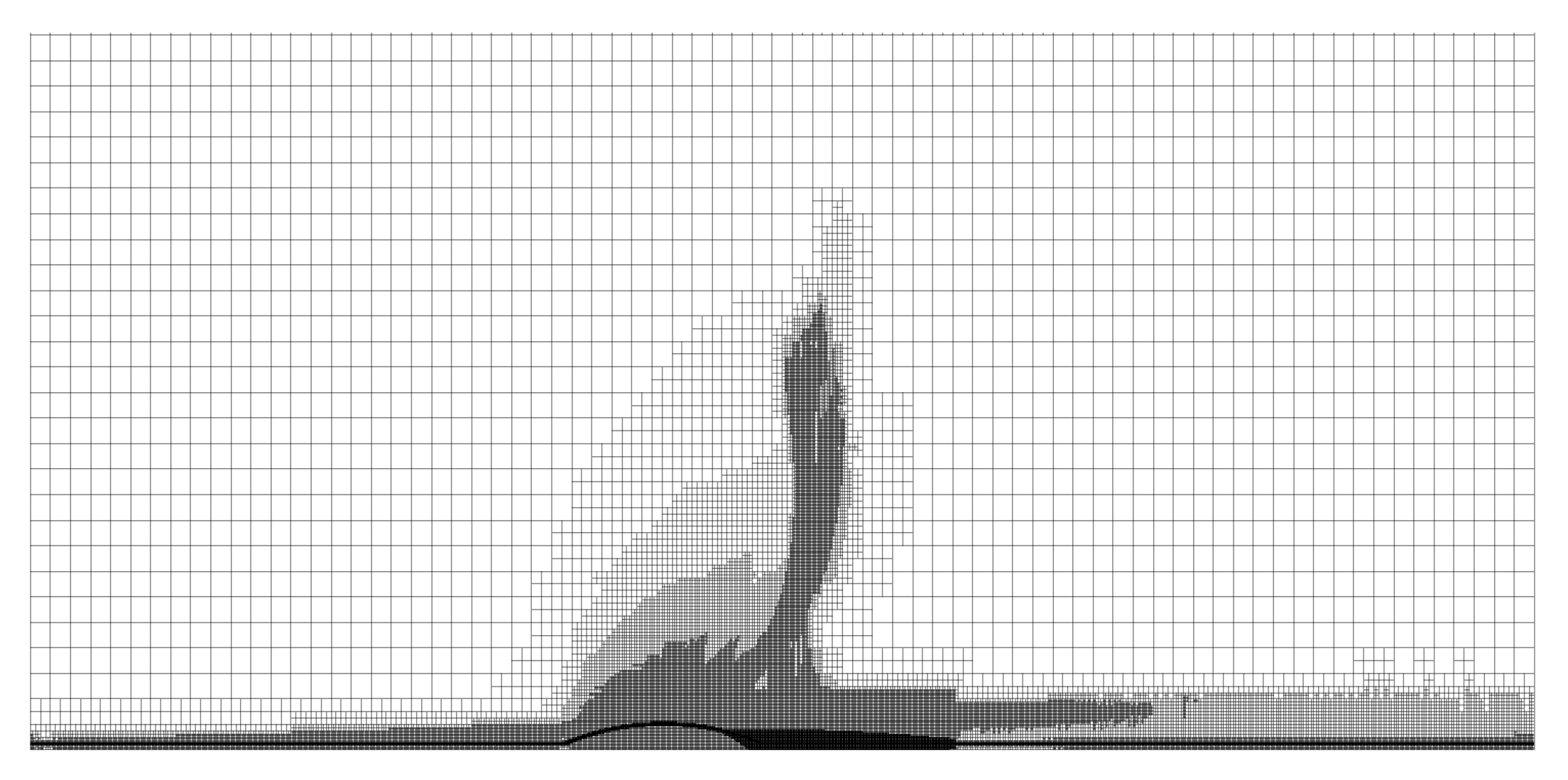
2.2. Mesh Refinement Scheme

In order to save computational costs, a kind of adaptive mesh refinement (AMR) technique is adopted to refine the mesh near the solid boundary or in some specific regions. Using the AMR method, each cell may be split into a given number of child cells. As shown in Figure 2, during a splitting process, a 2D cell gives birth in a Cartesian grid to four child cells and a 3D cell to eight child cells [20]. Two criteria are adopted to justify whether the splitting process is needed or not near the solid boundary.

$$Criterion1:\begin{array}{c}\frac{D_{wall}}{l_{level}}<T_V\end{array}$$

(3)

where $D_{wall}$ is the distance from the point being calculated to the solid boundary, $l_{level}$ the present mesh size of the cell, and $T_V$ the given threshold value.

$$Criterion2:\begin{array}{c}\left|Leve{l}_{center}-Leve{l}_{neighbor}\right|>1\end{array}$$

(4)

where $Leve{l}_{center}$ is the mesh level of the concerned cell, and $Leve{l}_{neighbor}$ is the mesh level of the neighbored cell. Provided $T_V=1$, it is shown in Figure 3 that cell 1 does not need refining treatment anymore, while cell 2 needs to be split based on criterion 1, cell 3 based on criteria 1 and 2, and cell 4 based on criterion 2.

In some cases, as variables or their gradients are changed dramatically in some special regions except those near the solid boundary, the necessary mesh refinement would be carried out in these regions based on criterion 3.

$$Criterion3:\begin{array}{c}\left|grad(\varphi )\right|>T_G\end{array}$$

(5)

where $\varphi$ is a general variable, $T_G$ the given threshold value.

Though the scale of the mesh is reduced efficiently by the AMR method, the discretization of the governing equations would have to be carried out among the different mesh levels. When the discretization is made, there are two kinds of situations for the Cell $i$ being calculated, marked by the black point and shown in Figure 4. One is that the related points are in the lower level or the coarse mesh, such as Cell $i-1$ shown on the left of Figure 4. The other one is that the related points are in the higher level or the finer mesh, such as Cell $i+1$ shown on the right of the figure. In this research, four neighbored points marked by the red triangles are used to substitute the Cell $i-1$ or Cell $i+1$ to estimate Cell i by the means of the multi-linear interpolation.

Furthermore, it is necessary to check the flux among the cell faces with a different mesh level at every calculation step. Once was non-conversation of the flux found, the necessary modification would be needed.

A moving solid boundary is a kind of boundary condition commonly found in some research, such as studies analyzing the performance of turbomachinery or fluid–structure interaction. At every time step, some points are involved in the fluid field from the solid, while some are rejected from the fluid field. As shown in Figure 5, when the time step proceeds from $T_n$ to $T_{n+1}$, the point $N$, which was in the solid at $T_n$, is then enrolled in fluid field at $T_{n+1}$. Thus, it is necessary to value the fresh fluid point $N$ before the calculation at the step $T_{n+1}$. If one draws a line through the point $N$ and makes it perpendicular to the solid boundary, the line intersects the solid boundary at the point marked BP, as shown in Figure 5. The mirror point of the BP named the extension point (EP) is found in the fluid field as the point $N$ is taken as a mirror. The variables’ value at the EP is determined by the neighbored points and the BP. Finally, the point $N$ is assigned based on the EP and boundary conditions. It is noted that the calculation accuracy would suffer from too many new enrolled fluid points in one time step. Thus, the displacement of the moving solid boundary in one time step should be controlled carefully.

2.3. Wall Function

Sometimes, the boundary layer very close to the solid wall is extremely thin, so the mesh refinement is not efficient enough to produce an accurate simulation. Therefore, the wall function can be used in these cases. In this research, referring to Tamaki’s model [12], a wall function scheme combined with the ghost cell IBM is introduced. First, the velocity component of the MP is resolved along the direction parallel to the tangential direction of the boundary line at the BP. The stress shear velocity can be calculated by the following Newton iteration:

$$u_{\tau }^1=u_{\tau }^0-\frac{u_{\tau }^0{U}^{+}(Y_{\mathrm{MP}}^{+})-u_{\mathrm{MP},t}}{U^{+}(Y_{\mathrm{MP}}^{+})+u_{\tau }^0{\left.(\partial U^{+}/\partial u_{\tau })\right|}_{Y^{+}=Y_{MP}^{+}}}$$

(6)

where $u_{\mathrm{MP},t}$ is the tangential component of velocity of the MP, $U^{+}$ is the dimensionless velocity near the wall, and $Y^{+}$ is the dimensionless wall distance. Additionally, the near-wall speed, $U^{+}\left(Y^{+}\right)$, can be estimated by the followed log-law distribution [21].

$$\begin{array}{l}{U}^{+}(Y^{+})=\overline{B}+c_1\log [{(Y^{+}+a_1)}^2+b_1^2]-c_2\log [{(Y^{+}+a_2)}^2+b_2^2]-\\ c_3\arctan [Y^{+}+a_1,b_1]-c_4\arctan [Y^{+}+a_2,b_2]\end{array}$$

(7)

Then, the tangential velocity component of the GP, $u_{\mathrm{GP},t}$, can be revised by the following formula:

$$u_{GP,t}=u_{\tau }{U}^{+}\left(Y_{MP}^{+}\right)$$

(8)

In this research, when the mesh level reaches 10 near the solid boundary but the $Y^{+}$ is still bigger than 50, the wall function goes into operation.

Based on the above-mentioned principles, we improved an in-house code [18]. In the code, the grid is numbered based on the mesh level number. The grid structure allows the refinement of the chosen cells without the regeneration of the entire mesh. In addition, each cell has the knowledge of its neighboring cells so that it is easy for discretized equations to be solved and the new refined grid to be maintained.

Meanwhile, unsteady and compressible Navier–Stokes (N-S) equations are used as the governing equations. The time derivative is discretized by an explicit scheme, the Adams–Bashforth scheme, with second-order accuracy. A five-order weighted essentially non-oscillatory scheme (WENO) is adopted to finish the spatial discretization process [18]. Additionally, a shear stress transport (SST) $k-\omega$ turbulence model is selected to close the Reynold-averaged Navier–Stokes simulation (RANS) equations.

3. Numerical Tests

3.1. Two-Dimensional Supersonic Inviscid Flow

The aim of the first test is to verify the calculation capacity of the IBM with the AMR technique for the analysis of the supersonic flow. The classic model, which consists of a circular-arc bump affixed to a cylinder aligned with the incident flow, is a kind of circular symmetric flow model and can be simplified as a 2D model. The model size is shown in Figure 6, which refers to the work of Bachalo [22]. The far-field boundary conditions are set on the left, right, and upper boundaries. Additionally, the Mach number ($M{a}_{\infty }=0.875$), static pressure ($p_{\infty }=1.013\times {10}^5 \mathrm{Pa}$), and the direction of velocity are provided on these boundaries.

The AMR technique is adopted near the solid boundary based on Criterion 1 and criterion 2, and the maximum mesh level is 10. Meanwhile, the mesh refinement is also carried out based on criterion 3 in some regions in which the density and velocity change dramatically. The final mesh generated by the AMR is shown in Figure 7.

The Mach number contour is shown in Figure 8. It is shown in the figure that the shock wave can be observed at about $x/C=0.7$, which agrees with the experimental data [22]. Additionally, the back-flowing zone is extended to $x/C=1.1$, which is consistent with the published numerical results from LES [23].

The pressure coefficient on the solid wall surface is compared in Figure 9. The pressure coefficient is defined as follows:

$$C_p=\frac{p-p_{\infty }}{\frac{1}{2}{\rho }_{\infty }{u}_{\infty }^2}$$

(9)

In the figure, the coefficient from the IBM is highly consistent with that from the CFL3D software [24]. All the same, there is a small difference between the experimental data and the series of numerical simulation results in the back-flowing region. It is thought that the error is mainly caused by three-dimensional effects in the experiments.

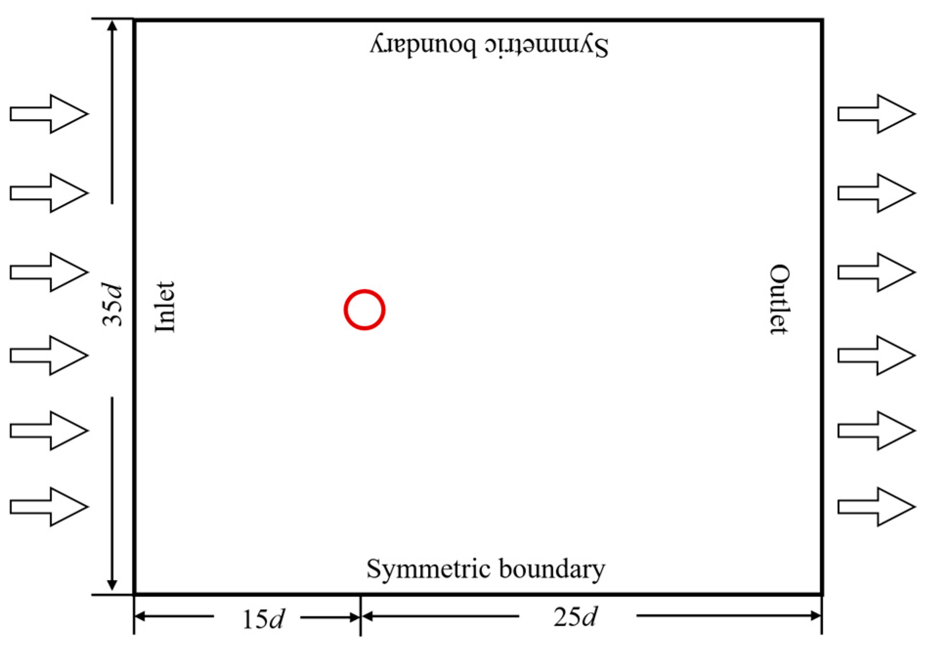
3.2. Flow around the Circular Cylinder

3.2.1. Low-Speed Flow

In the following test, a circular cylinder is placed in a chamber. The computation domain and the boundaries are shown in Figure 10. In this case, the Reynold number, $R{e}_d$, is provided at the inlet, reaching 100, 150 and 200, respectively.

The AMR technique is also used in the regions near the cylinder surface based on Criterion 1 and criterion 2, and the maximum mesh level is 7 in these regions. The velocity is adopted as a control variable to complete the mesh refinement in other regions based on criterion 3. The final mesh generated by the AMR is shown in Figure 11.

The vorticity contours under three $R{e}_d$ values are shown in Figure 12. In this figure, the famous Kármán Vortex Street can be observed in the downstream of the cylinder. It is due to the increase in the velocity that the vortex shedding process becomes more intensive with the increase in Reynold number; consequently, the intensity of vorticity increases.

The lift coefficient $C_l$ and the drag coefficient $C_d$ as well as Strouhal number St are usually used to investigate the calculation accuracy. They are defined using the following formulae:

$$C_l=F_l/(0.5\rho u_{\infty }^{2}d)$$

(10)

$$C_d=F_d/(0.5\rho u_{\infty }^{2}d)$$

(11)

$$St=f\cdot d/u_{\infty }$$

(12)

where $F_l$ and $F_d$ are the vertical component and the horizontal component of the aerodynamic force acting on the cylinder, which contribute to the pressure difference and the viscosity friction. $f$ is the frequency of $F_l$. $C_l$ and $C_d$ are estimated according to Equations (10) and (11) as shown in Figure 13. It is found that the force acting on the cylinder is obviously periodical, and the frequency of the $C_d$ is twice that of $C_l$, which has already been proven in many published materials. Moreover, the numerical results are compared with the experimental data [25] listed in

Table 1. Comparison of C_d and St.

Red	Cd (IBM)	Cd (EXP [25])	Cd Error%	St (IBM)	St (EXP [25])	St Error%
100	1.452	1.375	5.60	0.171	0.166	3.012
150	1.417	1.361	4.115	0.185	0.183	1.093
200	1.412	1.346	4.903	0.198	0.197	0.508

. The maximum error of the averaged $C_d$ between calculation and experiment is 5.6%, while the maximum error of St is only 3.0%.

3.2.2. Supersonic Flow

In order to validate the method further, the boundary condition is changed to supersonic flow, for example, $M{a}_{\infty }=1.7$, $R{e}_d=4\times {10}^5$. Concerning the influence of shock wave reflection, the far-field boundary condition is used to substitute the inlet, the outlet, and the symmetric boundary.

In the case of the low-speed flow, the AMR technique is also used to refine the mesh near the cylinder surface based on criterion 1 and criterion 2, but the maximum mesh level is 10 in these regions. The density is adopted as a control variable to complete the mesh refinement in other regions based on criterion 3. The final mesh generated by the AMR is shown in Figure 14. It is different from the mesh used in low-speed flow case (shown in Figure 11).

The Mach number contours are shown in Figure 15. A strong detached shock wave is captured upstream from the cylinder. The state of the flow is changed to subsonic through the shock wave and then quickly recovered to supersonic condition due to the circular surface of the cylinder. The flow separation, which is occurred at the rear part of the cylinder, can also be attributed to the circular surface. So, the phenomenon is observed that the back-flow region behind the separation point, which is surrounded by the supersonic flow; furthermore, a pair of symmetric shear layers are formed downstream of the cylinder. When the back-flow region is shrunken gradually in the wake, two parts of supersonic streams from the upper and lower cylinder surfaces collide, and two oblique shocks are produced. This flow pattern has been proven in many published works [26,27,28].

Additionally, the position of the separation point ${\theta }_{sep}$ and drag coefficient $C_d$ are listed in

Table 2. Comparison of the position of the separation point.

	${\theta }_{sep}$	$C_d$
Present IBM	111°	1.41
Bashkin et al. (Exp.) [26]	112°	1.43
De Palma et al. (IBM) [27]	111°	1.39
Yuan and Zhong (IBM) [28]	119°	1.45

. The results from our method are compared with those from experiments [26] and other IBM methods [27,28]. It is noted that $C_d$ from the numerical results agrees well with the experimental data. However, for ${\theta }_{sep}$, only the results from this paper and from reference [27] are consistent with the experimental data. The error between the experimental data and those from the reference [28] is around $7°$, which implies that the grid used in reference [28] is not fine enough to obtain the real convergent solution.

The computed pressure coefficient’s distribution along the surface of the cylinder is shown in Figure 16. The consistency between this paper and the reference [27] is so great that the two curves almost overlap. Meanwhile, both agree well with the experimental data, though the error is larger when $\theta$ ranges from $50°$ to $100°$. This error can be attributed to the difference between the two models.

3.3. Single Rotor Cascade of an Axial-Flow Compressor

A single row of rotor cascade is adopted to validate the method used in the cases with the moving solid boundaries. The parameters related to the rotor cascade are listed in

Table 3. The parameters of the rotor cascade [29].

Parameter	Value
Rotation speed (rpm)	4010
Pressure ratio	1.15
Volume coefficient	0.0783
Rotor tip difference ratio ($\delta /r_{hub}$)	0.001
Hub ratio	0.91
Ma (blade tip of the rotor)	0.698
Blade number	93

. Additionally, the numerical simulation model is shown in Figure 17. The inlet surface is in the front of the rotor cascade, which is the position for the measurement in the experiments [29]. The total pressure and total temperature are provided on the inlet surface, and both are determined by the measured data. The outlet surface is far away from the trailing edge of the blades, about seven times $C_{ax-R1}$ (the axial length of the airfoil). The static pressure is assigned to the outlet surface. It is noted that on the shroud, the case treatment is carried out to enlarge the operating range [29].

The AMR technique is adopted in the region near the solid boundaries. The maximum mesh level is as much as 10 in these regions. The final grid generated by the AMR is shown in Figure 18. The total grid number is about $3.2\times {10}^9$. In order to control the number of the new enrolled fluid points, the $\Delta t$ is set to as much as $1.2\times {10}^{-7}$ s.

Meanwhile, the commercial software, CFX [29], is used to make comparisons. The calculation model (full circumferential annulus) and boundary conditions are all the same as those mentioned in the above paragraph. The number of the body-fitted grid is about $5\times {10}^8$. SST $k-\omega$ is used as the turbulence model. For the spatial discretization, the high-resolution method [30] is used as the convection term. For the time discretization, the dual-time scheme is adopted. The pseudo time step is set to 20, and the physical time $\Delta t$ is $6.7\times {10}^{-6}$ s, which is 1/24 of the blade passing time (BPT). The total simulation time is $3.2\times {10}^{-4}$ s, which corresponds to two times the rotating time (RT). The grid independence setting and result are shown in

Table 4. The grid setting for grid independence verification.

Grid	Grid Number (×108)
Grid 1	1
Grid 2	2.5
Grid 3	5
Grid 4	8
Grid 5	12

and Figure 19, which show simulations under the peak efficiency condition (PE). With the increase in grid number, the efficiency tends to stay at a fixed value. From grid 3 to grid 4, the efficiency only varies by 0.0003, which indicates that grid 3 is sufficient and will be chosen for the following analysis.

3.3.1. Overall Performance

In Figure 19, the overall performance obtained withthe IBM is compared with that in experiments and with CFX. The normalized mass flow is defined as the mass flow divided by the choke flow, and the total pressure ratio is defined as the outlet total pressure divided by the inlet total pressure ratio. For the adiabatic efficiency, it is defined as

$$\eta =\frac{{(\frac{P_{Tout}}{P_{Tin}})}^{\frac{\gamma -1}{\gamma }}-1}{\frac{T_{Tout}}{T_{Tin}}-1}$$

where $P_{Tin}$/$P_{Tout}$ are the total pressure at the inlet/outlet boundary; $T_{Tin}$/$T_{Tout}$ are the total temperature at the inlet/outlet boundary; and $\gamma$ is the heat capacity ratio.

It is found that the performance from the IBM is more consistent with the experimental data than those from CFX. At the peak efficiency point (PE), the efficiency of IBM is greater than that of the experiment by as much as 0.23%, while that of CFX is as much as 0.569% lower (as shown in Figure 20a). In Figure 20b, the difference between the total pressure ratios from IBM and those from the experiment becomes more obvious when the working conditions are close to the near-stall point (NS). All the same, these two series of total pressure ratios show good agreement under the left working conditions. So, based on the figure, it is believed that the results from the IBM are more accurate than those from CFX.

3.3.2. PE Working Condition

At the PE point, a comparison of the span-wise distribution of the efficiency and the total pressure ratio is shown in Figure 21. It can be observed from Figure 21a that both results from the IBM and CFX are consistent with the experimental data from the hub up to 60% of the blade height. However, in the blade’s top region, the maximum difference in efficiency between CFX and the experiments is about 2.98%, while for the IBM, it is only 0.97%. The same situation can be found in Figure 21b.

To compare the results further, the static pressure contours from four sections are shown in Figure 22. Four case treatment grooves are arranged in a flow passage so that the four sections, S1, S2, S3, and S4, are selected according to these grooves. It is found in these contours that the distributions from the IBM and CFX are similar to each other except in the region near the blade’s top. In the blade’s top region, the data exchange at the interface between rotational cells and static cells for the body-fitted grid is unavoidable. This gives rise to abrupt change and destroys the continuity of the gradient of some parameters. From the CFX result, due to the data exchange between the static grooves and the moving flow passage, the pressure continuity cannot be guaranteed. Usually, the low-pressure region in the groove is enlarged somewhat so that more fluid enters into the groove. Based on the calculation, the incidence flow from CFX is larger than that from the IBM by as much as 4.1%. Once the incidence flow increases, the aerodynamic loss also increases, and efficiency is negatively effected. This is why the efficiency of CFX is lower than that of the IBM in the region near the blade’s top.

3.3.3. NS Working Condition

The simulation accuracy near the NS working conditions is one of the most important criteria for validating a method or a programmed code. The span-wise comparison of the efficiency and the total pressure ratio’s distribution at the NS point is shown in Figure 23. As a whole, the results from the IBM are still better than those from CFX, though the accuracy of the IBM is decreased a little bit compared with that under the PE working condition. The maximum efficiency difference between the IBM and the experiments is about −1.857% at about 80% of the blade height, and the maximum difference for the total pressure ratio is about −0.845%.

The results of spectrum analysis based on the FFT are shown in Figure 24. The initial static pressure signals were measured in front of the rotor cascade. It is found from the experimental data that the main frequencies include the by-pass frequency (BPF), the doubled BPF, and the tripled BPF. Besides these frequencies, there is another important frequency, called rotational–instable frequency (RF). The RF is mainly caused by the circumferential disturbance due to the rotation, which is believed to have a close connection to the stall inception [31]. A RF is about 0.843 BPF measured in experiment, while it is 0.831 BPF from the IBM and 0.865 BPF from CFX, marked A in Figure 24. The two numerical methods seem to have the same accuracy in this respect. It is also observed that unlike CFX, the IBM can still provide detailed information in the low-frequency band (marked B in Figure 24), which shows good consistency with the experimental data. This kind of detailed information would benefit to stall research and analysis.

3.3.4. Discussion

For rotational fluid machinery, the body-fitted mesh is a traditional scheme used for numerical simulation. When the model geometry is complex, it is not an easy task to achieve a fine body-fitted mesh. Plenty of studies have focused on how to improve factors of mesh quality such as orthogonality, aspect ratio, and so on. However, in the IBM, this kind of work is saved by the immersed boundary. In addition, for the traditional body-fitted mesh, the calculation domain is usually divided into two parts: the rotational region and the static region. So, the data exchange between two regions is unavoidable. This gives rise to the distortion and the loss of the data and leads to unavoidable calculation errors, especially in the unsteady calculation. In the IBM, no additional strategy for data exchange is needed, and some detail information can be reserved successfully.

Flow within turbomachinery has some typical characteristics, such as a high Reynold number, 3D features, unsteady flow, and so on. Additionally, the calculation strategy in regions near the blades, hub, and shroud is very important for the estimation of the machine’s performance. So, in these regions, the characteristic length of the grid should be small enough. This is beneficial for the body-fitted mesh because of its flexible mesh refinement scheme. However, in the IBM, the mesh refinement brings about a sharp increase in the grid number, though the AMR technique may be used to mitigate this situation somewhat. Moreover, for dealing with the moving solid boundary, the time step of the IBM is smaller than that adopted in the body-fitted mesh scheme in order to control the number of newly involved fluid points. Thus, the calculated consumption of the IBM is so high that its practical application is not efficient and cannot be realized authentically at present. However, it is believed that when the calculation source no longer needs to be considered as a barrier to the development of computer technology, the IBM will have wide applications in the field of numerical simulation.

4. Conclusions

The basic aim of this research is to find a method by which compressible flow can be estimated more accurately and efficiently. To this end, a discrete cell method, or ghost cell IBM, was introduced into an in-house flow solver, which is believed to be suitable for numerical simulation of the compressible flow. Moreover, particular effort has been focused on the mesh refinement scheme, and the AMR technique was adopted to avoid unnecessary increases in the grid number. Additionally, a wall function was modified according to the IBM. We may draw the following conclusions on current state-of-the-art methodologies for calculating compressible flow, demonstrating the perception of researchers in the field of numerical simulation:

• With the help of the AMR technique and the wall function, it is verified by three cases that the ghost cell IBM can be applied to numerical simulation of compressible flow. Compared with the results based on the body-fitted mesh, more detailed and useful information is obtained via the IBM, though calculation costs are a little higher.
• Based on the AMR presented in this paper, the scale of the mesh adopted in the IBM is controlled, and calculation efficiency is subsequently increased. The final mesh is determined by the criteria. As the criteria are different, the final mesh is different, even if the same geometry and calculation domain are used.
• The wall function is a very useful tool in the calculation of turbulence. Combined with the IBM, it can increase the calculation efficiency further when the boundary layer is extremely thin.

References

1. Gong, Z.-X.; Lu, C.-J.; Huang, H.-X. Immersed boundary method and its application. Chin. Q. Mech. 2007, 28, 353–362. (In Chinese) [Google Scholar]
2. Peskin, C.S. The immersed boundary method. Acta Numer. 2002, 11, 479–517. [Google Scholar] [CrossRef]
3. Peskin, C.S. The fluid dynamics of heart valves: Experimental, theoretical, and computational methods. Annu. Rev. Fluid Mech. 1982, 14, 235–259. [Google Scholar] [CrossRef]
4. Zhu, L.; Peskin, C.S. Interaction of two flapping filaments in a flowing soap film. Phys. Fluids 2003, 15, 1954–1960. [Google Scholar] [CrossRef]
5. Xu, D.; Xu, H.; Chun, N.; Yang, H.; Zhang, B. Direct-forcing immersed boundary method for incompressible viscous flow and its software implementation. Chin. J. Comput. Mech. 2019, 36, 520–527. (In Chinese) [Google Scholar]
6. Lai, M.C.; Peskin, C.S. An immersed boundary method with formal second-order accuracy and reduced numerical viscosity. J. Comput. Phys. 2000, 160, 705–719. [Google Scholar] [CrossRef]
7. Mittal, R.; Iaccarino, G. Immersed boundary methods. Annu. Rev. Fluid Mech. 2005, 37, 239–261. [Google Scholar] [CrossRef]
8. Majumdar, S.; Iaccarino, G.; Durbin, P. RANS solvers with adaptive structured boundary non-conforming grids. Annu. Res. Briefs 2001, 1, 179. [Google Scholar]
9. Iaccarino, G.; Verzicco, R. Immersed boundary technique for turbulent flow simulations. Appl. Mech. Rev. 2003, 56, 331–347. [Google Scholar] [CrossRef]
10. Ghias, R.; Mittal, R.; Dong, H. A sharp interface immersed boundary method for compressible viscous flows. J. Comput. Phys. 2007, 225, 528–553. [Google Scholar] [CrossRef]
11. Takahashi, Y.; Imamura, T. High Reynolds number steady state flow simulation using immersed boundary method. In Proceedings of the 52nd Aerospace Sciences Meeting, National Harbor, MD, USA, 13–17 January 2014; p. 0228. [Google Scholar]
12. Tamaki, Y.; Harada, M.; Imamura, T. Near-wall modification of Spalart–Allmaras turbulence model for immersed boundary method. AIAA J. 2017, 55, 3027–3039. [Google Scholar] [CrossRef]
13. Constant, B.; Péron, S.; Beaugendre, H.; Benoit, C. An improved immersed boundary method for turbulent flow simulations on Cartesian grids. J. Comput. Phys. 2021, 435, 110240. [Google Scholar] [CrossRef]
14. Ye, H.; Chen, Y.; Maki, K. A discrete-forcing immersed boundary method for turbulent-flow simulations. Proc. Inst. Mech. Eng. Part M J. Eng. Marit. Environ. 2021, 235, 188–202. [Google Scholar] [CrossRef]
15. Luo, K.; Zhuang, Z.; Fan, J.; Haugen, N.E.L. A ghost-cell immersed boundary method for simulations of heat transfer in compressible flows under different boundary conditions. Int. J. Heat Mass Transf. 2016, 92, 708–717. [Google Scholar] [CrossRef]
16. Chi, C.; Abdelsamie, A.; Thévenin, D. A directional ghost-cell immersed boundary method for incompressible flows. J. Comput. Phys. 2020, 404, 109122. [Google Scholar] [CrossRef]
17. Zhang, Y.; Fang, X.; Zou, J.; Shi, X.; Ma, Z.; Zheng, Y. Numerical simulations of shock/obstacle interactions using an improved ghost-cell immersed boundary method. Comput. Fluids 2019, 182, 128–143. [Google Scholar] [CrossRef]
18. Liu, X.; Yang, B.; Ji, C.; Chen, Q.; Song, M. Research on the Turbine Blade Vibration Base on the Immersed Boundary Method. ASME J. Fluids Eng. 2018, 140, 061402. [Google Scholar] [CrossRef]
19. Yan, C.; Huang, W.-X.; Cui, G.-X.; Xu, C.; Zhang, Z.-S. A ghost-cell immersed boundary method for large eddy simulation of flows in complex geometries. Int. J. Comput. Fluid Dyn. 2015, 29, 12–25. [Google Scholar] [CrossRef]
20. Schmidmayer, K.; Petitpas, F.; Daniel, E. Adaptive Mesh Refinement Algorithm Based on Dual Trees for Cells and Faces for Multiphase Compressible Flows. J. Comput. Phys. 2019, 388, 252–278. [Google Scholar] [CrossRef]
21. Allmaras, S.R.; Johnson, F.T. Modifications and clarifications for the implementation of the Spalart-Allmaras turbulence model. In Proceedings of the 7th International Conference on Computational Fluid Dynamics (ICCFD7), Big Island, HI, USA, 9–13 July 2012. [Google Scholar]
22. Bachalo, W.D.; Johnson, D.A. Transonic, turbulent boundary-layer separation generated on an axisymmetric flow model. AIAA J. 1986, 24, 437–443. [Google Scholar] [CrossRef]
23. Iyer, P.S.; Park, G.I.; Malik, M.R. Wall-modeled large eddy simulation of transonic flow over an axisymmetric bump with shock-induced separation. In Proceedings of the 23rd AIAA Computational Fluid Dynamics Conference, Denver, CO, USA, 5–9 June 2017; p. 3953. [Google Scholar]
24. Jespersen, D.C.; Pulliam, T.H.; Childs, M.L. Overflow Turbulence Modeling Resource Validation Results; NASA Technical Report; NASA AMES Research Center: Mountain View, CA, USA, 2016. [Google Scholar]
25. Potter, M.C.; Wiggert, D.C. Schaum’s Outline of Fluid Mechanics; McGraw-Hill Education: New York, NY, USA, 2016; ISBN 13 978-1305635173. [Google Scholar]
26. Bashkin, V.A.; Vaganov, A.V.; Egorov, I.V.; Ivanov, D.V.; Ignatova, G.A. Comparison of calculated and experimental data on supersonic flow past a circular cylinder. Fluid Dyn. 2002, 37, 473–483. [Google Scholar] [CrossRef]
27. De Palma, P.; De Tullio, M.D.; Pascazio, G.; Napolitano, M. An immersed-boundary method for compressible viscous flows. Comput. Fluids 2006, 35, 693–702. [Google Scholar] [CrossRef]
28. Yuan, R.; Zhong, C. An immersed-boundary method for compressible viscous flows and its application in the gas-kinetic BGK scheme. Appl. Math. Model. 2018, 55, 417–446. [Google Scholar] [CrossRef]
29. Zhu, G.M. A Study of Inlet Distortion Influence and Stall Margin Enhancement Method in Axial Compressor. Ph.D. Thesis, Shanghai Jiaotong University, Shanghai, China, 2022. (In Chinese). [Google Scholar]
30. Barth, T.; Jespersen, D. The design and application of upwind schemes on unstructured meshes. In Proceedings of the 27th Aerospace Sciences Meeting, Reno, NV, USA, 9–12 January 1989. [Google Scholar]
31. Hewkin-Smith, P.; Pullan, G. The role of tip leakage flow in spike-type rotating stall inception. ASME J. Turbomach. 2019, 141, 061010. [Google Scholar] [CrossRef]
Figure 1. Sketch of the ghost cell immersed boundary method.
Processes 12 01182 g001
Figure 2. Sketch of the Cartesian grid refinement method [20].
Processes 12 01182 g002
Figure 3. Sketch of mesh refinement criteria.
Processes 12 01182 g003
Figure 4. Difference scheme in ASR.
Processes 12 01182 g004
Figure 5. Fresh fluid nodes due to the boundary motion.
Processes 12 01182 g005
Figure 6. Computation domain and boundary conditions.
Processes 12 01182 g006
Figure 7. Mesh generated by the AMR.
Processes 12 01182 g007
Figure 8. Mach number contours and streamlines.
Processes 12 01182 g008
Figure 9. Wall pressure coefficient (Exp. results referred to Ref. [22], CFL3D results referred to Ref. [24]).
Processes 12 01182 g009
Figure 10. Scheme of computation domain and boundaries.
Processes 12 01182 g010
Figure 11. Mesh generated by the AMR.
Processes 12 01182 g011
Figure 12. Vorticity normal to the plane.
Processes 12 01182 g012
Figure 13. Lift coefficient and drag coefficient ( Re d = 100).
Processes 12 01182 g013
Figure 14. Mesh generated by the AMR.
Processes 12 01182 g014
Figure 15. Mach number contours.
Processes 12 01182 g015
Figure 16. Pressure coefficient’s distribution along the surface of the cylinder (Bashkin’s data referred to Ref. [26], and De Palma’s data referred to Ref. [27]).
Processes 12 01182 g016
Figure 17. Scheme of the simulation model.
Processes 12 01182 g017
Figure 18. Mesh generated by the AMR.
Processes 12 01182 g018
Figure 19. Grid independence verification.
Processes 12 01182 g019
Figure 20. Comparisons of overall performance.
Processes 12 01182 g020
Figure 21. Span-wise comparisons of performance at the PE point.
Processes 12 01182 g021
Figure 22. Static pressure contours at the PE point.
Processes 12 01182 g022
Figure 23. Span-wise comparisons of performance at the NS point.
Processes 12 01182 g023
Figure 24. Pressure spectrum in front of the leading edge of the rotor cascade at the NS point.
Processes 12 01182 g024