Analysis of Fault Influence on Geostress Perturbation Based on Fault Model Test

Abstract

The distribution of the geostress field in reservoirs holds significant implications for the precise exploration and efficient development and utilization of oil and gas resources, especially in deep strata regions where faults are prevalent. Geological structural movements in these deep strata regions exacerbate the complexity of geostress field distributions. To elucidate the perturbation of the geostress field in deep reservoirs caused by faults, this study initially conducted a series of physical model tests on single fault dislocation, employing digital image correlation techniques to capture the displacement fields of various types of fault dislocations. Subsequently, a numerical model of the fault interface element was established, and fault element parameters were determined through sensitivity analysis and trial calculation. This study further analyzed the perturbation of the geostress field using this numerical model. Finally, a multi-fault numerical simulation model was constructed to clarify the perturbations in the regional geostress field under the influence of multiple faults. The results indicate that the geostress perturbation range under the action of multiple faults spans from 183.06 to 310.06 m.

1. Introduction

The determination of geostress magnitude and distribution is of the utmost importance in the field of petroleum exploration and development. In the early stages of oil and gas field development, geostress was the basis for mining design, well location planning, and optimized production strategies; during drilling operations, geostress is essential for assessing and maintaining wellbore stability, preventing collapse, and ensuring a safe and efficient drilling process [1,2]. Deep oil and gas reservoirs, being subject to multiple episodes of mineralization during their formation, commonly exhibit faulting and other unfavorable geological features, which further complicates the prediction of geostress patterns within these reservoirs [3]. Consequently, it is vital to analyze the influence of faults on geostress perturbations, particularly in regions prone to faulting, as this information is instrumental in the development of oil and gas reservoirs.

Due to constraints imposed by geological and operational conditions, conducting field tests presents significant challenges and difficulties. This is especially true in areas such as deep oil and gas reservoirs, which the equipment cannot reach. To overcome these limitations, physical model tests based on similarity theory are commonly employed to simulate field conditions and explore the displacement patterns of change in the research subject. Displacements and deformations in strata caused by faults are primarily controlled by internal and external factors. Internal factors mainly refer to the geometric characteristics of the fault [4,5,6], while external factors include stress conditions and the elastic modulus of the stratum [7]. Regions with a history of tectonic activity often exhibit inherited faults [8], which not only have an impact on the regional tectonic distribution but also evolve during new tectonic movements to form complex fault systems [9]. The interaction of multiple faults within such systems can result in intricate combined effects. Large-scale model tests on multiple strike-slip faults demonstrated the occurrence of nonlinear linkage displacement within the fault zone under the combined action of multiple faults [10]. Wet clay physical models can be used to analyze the impact of inherited faults with different geometrical shapes and orientations on the development of new extensional structures within a basin [11].

Field geostress data reveal that fault activity has a significant influence on the continuity and structural integrity of rock masses, thereby affecting the distribution of geostress [12,13,14]. Numerical simulation methods, utilizing geological data, seismic data, and drilling data such as borehole logs and core samples, can provide a quantitative analysis of geostress field perturbations caused by faults. The finite element method and the finite difference method are the main numerical simulation methods for geostress field disturbances near fault zones [15,16,17,18,19,20]. The discrete element method can also be used to analyze the relationship between fault activity and three-dimensional geostress [21]. Summarizing previous numerical simulations of geostress fields in fault-prone regions reveals that multiple factors, including the size of the fault, boundary conditions, dislocation modes, and physical parameters of the rock mass, significantly impact geostress [21,22,23,24,25].

While the referenced literature has explored geostress perturbations in fault-prone regions, physical model tests have primarily focused on fault displacement and deformation, lacking a quantitative analysis of the impact of faults on geostress perturbations. Furthermore, numerical analysis methods have not adequately incorporated test data to calibrate internal fault factors. Therefore, this study aims to address these gaps by establishing a physical model based on similarity theory, which simulates actual faults, to conduct fault dislocation tests. By integrating digital image correlation analysis and numerical simulation methods, this study aims to deduce the influence of single fault dislocation on internal geostress perturbations within the model. The main factors contributing to geostress perturbation will be analyzed, and a fault stress perturbation analysis model will be developed. Ultimately, this research aims to elucidate the characteristics of various faults’ impacts on geostress under deep stratum conditions.

2. Fault Physical Model Test

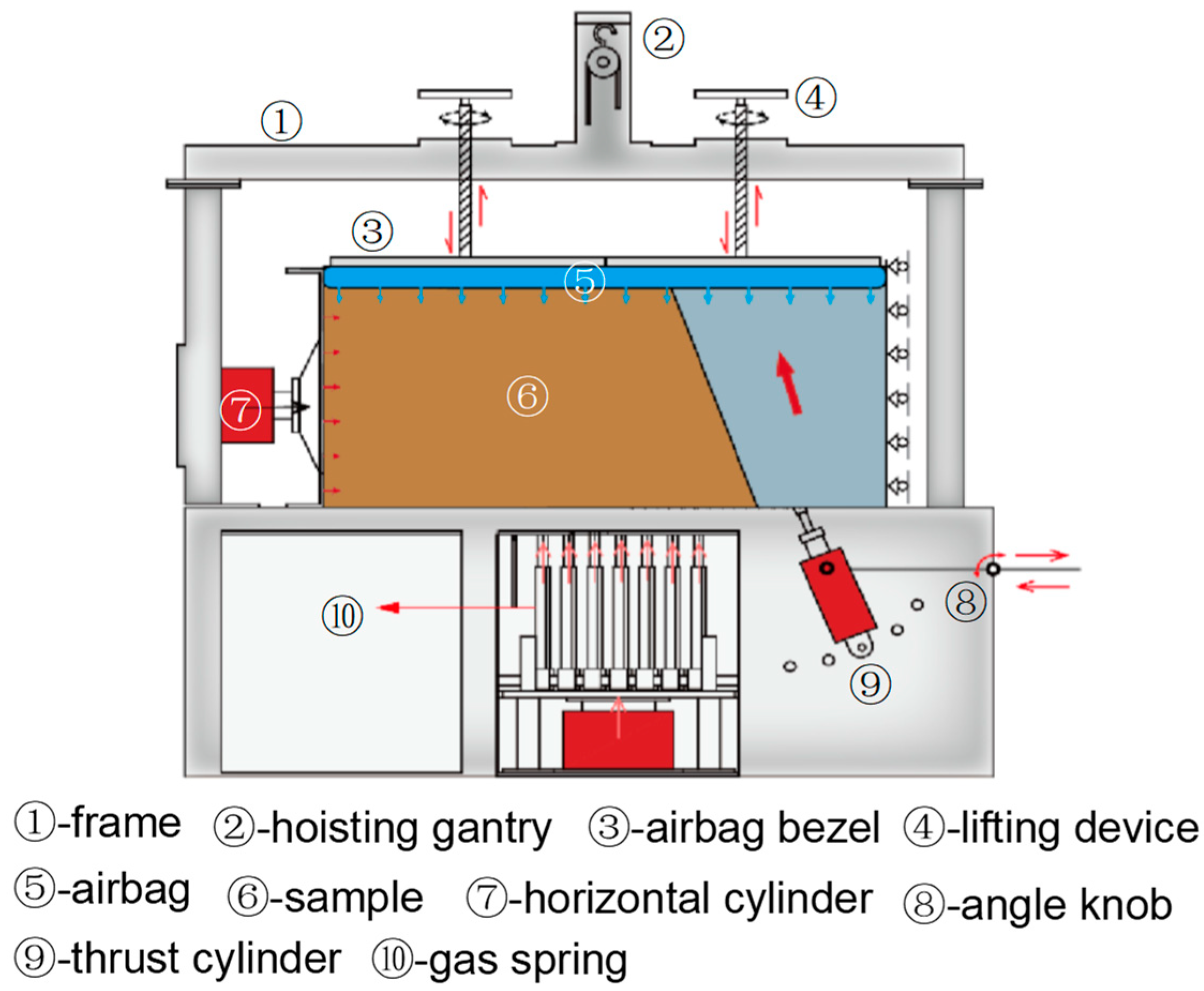
The physical model test of fault dislocation is based on similarity theory, referencing the actual mechanical parameters of reservoirs and the geometric elements of faults to design an indoor test scheme corresponding to actual faults. This approach explores the impact of fault dislocation on strata through indoor physical models. The physical model test in this article is based on three actual faults: F1 is a reverse fault with a dip angle of 55°~70°; F2 is a strike-slip fault with a dip angle of 85°~90°; F3 is a reverse fault with a dip angle of 70°~80°; the maximum principal stress within the reservoir range is 96.05~108.59 MPa; and the minimum principal stress range is 69.96~82.04 MPa. The test is divided into four parts: the selection of the similarity ratio and configuration of similar materials; the construction of the fault physical model; the monitoring of the fault dislocation process; and the processing of the test results.

2.1. Test Equipment

This test utilizes the fault dislocation simulation test platform under triaxial stress, independently developed by the Institute of Rock and Soil Mechanics, Chinese Academy of Sciences. The overall dimensions of the test apparatus are 2.2 m × 1.2 m × 2.2 m (length × width × height), with the internal model dimensions being 1.5 m × 0.6 m × 0.6 m (length × width × height). The equipment is primarily composed of ten parts: the external frame, hoisting gantry, airbag bezel, lifting device, airbag, sample, horizontal cylinder, angle knob, thrust cylinder, and gas spring. The external frame provides support and reaction force for the horizontal hydraulic cylinder and airbag baffle. The angle knob allows for the adjustment of the dislocation hydraulic cylinder’s angle to simulate different fault dislocation angles, while the gas spring provides flexible loading to ensure the continuity of displacement between the two sides of the fault during the dislocation process. One side of the fault dislocation simulation test platform is equipped with a customized, thickened transparent acrylic baffle, allowing for the observation and recording of the internal deformation of the model during the fault dislocation test (Figure 1).

The dislocation loading system is powered by a dislocation hydraulic cylinder, capable of providing a maximum dislocation load of 50 kN, with a maximum dislocation formation of 100 mm. By adjusting the angle knob, the loading direction of dislocation can be changed to simulate fault modes at different angles ranging from 45° to 90°. The geostress loading system comprises two parts: a hydraulic loading system and a pneumatic loading system. The maximum loading capacity of the hydraulic cylinder can provide a pressure of 3 MPa, with a maximum stroke of 100 mm; the airbag’s ultimate pneumatic parameter is 0.5 MPa, with a maximum compression amount of 80 mm. During the test, three-dimensional active geostress loads can be applied by placing airbags at the top and sides of the specimen, combined with the loading of the horizontal hydraulic cylinder, thereby simulating two types of stress boundary conditions: strike-slip faults and reverse faults.

2.2. Similarity Coefficient

The physical model test method involves studying scaled-down replicas of real-world structures, ensuring that the model accurately replicates the geometric shape, motion, and mechanical behavior of the actual structure. This allows the extrapolation of test results from the model to the real structure. In this study, the boundary stress similarity ratio is determined based on the relationship between the stress conditions in the actual geological environment and the loading capacity of the test equipment used to simulate these conditions. With the maximum principal stress in the actual strata being 110 MPa and the test boundary stress airbags’ maximum pneumatic pressure at 0.5 MPa, the boundary stress similarity ratio needed to satisfy the loading conditions is calculated to be greater than 220:1. Considering a reasonable margin for the test system, the boundary stress similarity ratio is set at 240:1. In specific model tests, the unit weight similarity ratio coefficient is set at 1:1, indicating that the density of the model material is the same as that of the prototype rock. Consistency is maintained in the stress similarity ratio, geometric similarity ratio, elastic modulus similarity ratio, and boundary stress similarity ratio (240:1 in this article), ensuring the model’s similarity to the prototype in all aspects. Moreover, the fault dislocation displacement similarity ratio is consistent with the geometric similarity ratio, maintaining the model’s dynamic behavior similarity to the prototype (

Table 1. Similar proportion coefficient.

Category	Similarity Parameters	Similarity Coefficient	Similarity Relationship
Density	Cγ	1	/
Geometry	CL	240	CL = Cσ/Cγ
Stress	Cσ	240	Cσ = CLCγ
Elastic modulus	CE	240	Cσ = CECε
Boundary stress	Cp	240	CE = Cp
Poisson’s ratio	Cν	1	Cν = Cε
Strain	Cε	1	/

Note: C_γ is the density similarity ratio, C_L is the geometric similarity ratio, C_σ is the stress similarity ratio, C_E is the elastic modulus similarity ratio, C_p is the boundary stress similarity ratio, C_ν is the Poisson’s ratio similarity ratio, and C_ε is the strain similarity ratio.

).

2.3. Similar Model

Based on the similarity coefficient determined above and combined with the mechanical parameters of the target reservoir rock mass, river sand and diatomite are selected as the main materials to configure similar materials. The specific material ratio is as follows: river sand–diatomite–cement–emery–water = 70%:15%:3%:5%:7%. The mechanical parameters of similar materials and reservoir rock mass are shown in

Table 2. Material mechanical parameters.

Material Type	Severity (kN/m3)	Elastic Modulus (GPa)	Poisson’s Ratio
Actual rock mass	23.9	26.80	0.20
Similar materials	23.2	0.11	0.20

Note: Similar coefficients of similar materials are as follows: C_γ = 1.03, C_E = 243.64, and C_ν = 1.

.

Incorporating the information on fault dip angles, three sets of fault dislocation physical model test schemes are determined: (1) 90° strike-slip fault dislocation test scheme; (2) 60° reverse fault dislocation test scheme; (3) 75° reverse fault dislocation test scheme. The fault’s hanging wall and footwall are constructed using a zoned paving approach, establishing fault planes at the aforementioned angles between different model upper and lower blocks, simulating the spatial distribution of faults within the reservoir (Figure 2).

Based on the specific proportions of the similar materials, the model is constructed using a zoned paving method as follows: (1) Construct and secure the fault mold according to the model setup requirements, dividing the model into passive and active block zones. (2) Lay the passive block from the bottom upwards, which, in this article, refers to the lower block of the reverse fault, compacting every 10 cm and measuring the levelness of the layer to ensure the compactness and uniformity within the similar model. (3) After the passive block is laid, remove the fault mold and level the prefabricated fault surface, and then lay the active block, which, in this article, refers to the upper block of the reverse fault, compacting every 10 cm and measuring the levelness of the layer until the entire model is laid. (4) Once the model casting is complete, remove the side limit steel plates of the model and install airbags on the sides and top of the model. Leave the model at room temperature (20 °C) for 7 days until it consolidates.

2.4. Test Process

Different fault dislocation physical model tests have varying boundary stress conditions: In the reverse fault model, the maximum horizontal principal stress is σ₁, the vertical principal stress is σ₃, and the minimum horizontal principal stress is σ₂. The principal stress directions in the physical model correspond to the actual directions. In the strike-slip fault model, the maximum horizontal principal stress is σ₁, the minimum horizontal principal stress is σ₃, and the vertical principal stress is σ₂. Due to the directional limitations of fault dislocation in this physical model test, the strike-slip fault dislocation direction is vertical. Therefore, in the physical model, the vertical principal stress is σ₁, the maximum horizontal principal stress is σ₂, and the minimum horizontal principal stress is σ₃. The specific boundary stress loading conditions are illustrated in Figure 3. and the movement direction of the active block on the right side of the fault plane is indicated by the blue arrow.

Based on the boundary stress similarity ratio, the boundary stress magnitudes for the fault dislocation simulation test are calculated, resulting in σ₁ = 0.42 MPa, σ₂ = 0.40 MPa, and σ₃ = 0.32 MPa. The dislocation distance for the physical model test refers to the actual fault displacement, calculated according to the geometric similarity ratio, establishing a displacement of 50 mm for all three faults. The fault dislocation process employs quasi-static loading to prevent the accumulation and release of energy inherent in dynamic loading. Quasi-static loading requires the material strain rate in the test to be between 10⁻⁵ s⁻¹ and 10⁻¹ s⁻¹, from which the fault dislocation rate in the physical model test is calculated to be 1 mm/min.

Throughout this test, a SONY PXW-FS5K digital CCD camera (Tokyo, Japan) was utilized to capture the entire process of the fault dislocation test with a resolution of 3840 (horizontal) × 2160 (vertical) pixels at 30 frames per second. The image data were analyzed using digital image correlation (DIC) with an open-source MATLAB-based program, NCORR v1.14.0.0. Due to the compression and deformation experienced by the active block, only the displacement perturbations within the passive block under fault dislocation were analyzed. The analysis region (Region of Interest) is depicted as shown in Figure 4. To ensure effective DIC analysis, preprocessing adjustments were made, using a subset radius of 60 pixels and a grid interval of 5 pixels as the computational parameters for the digital image correlation analysis.

During the test, boundary stress is applied to the top and sides of the model using the expansion of air bladders, while horizontal loading is provided by the extension and retraction of hydraulic cylinders. To ensure the stability and safety of the pneumatic loading, both the overflow valve and the pneumatic control valve are opened during loading. The stress is applied according to the preset loading levels and maintained at a constant pressure once the desired value is reached.

After the boundary stress loading is completed, the displacement loading of the active block is performed using a thrust cylinder according to the requirements of quasi-static loading. The loading is carried out in cycles of 10 mm each, for a total of 5 cycles.

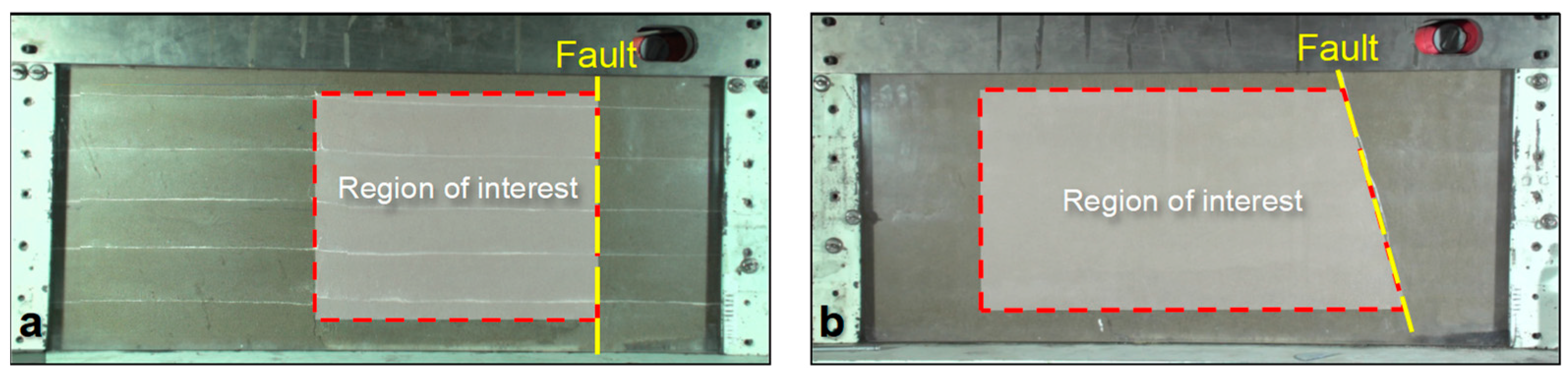
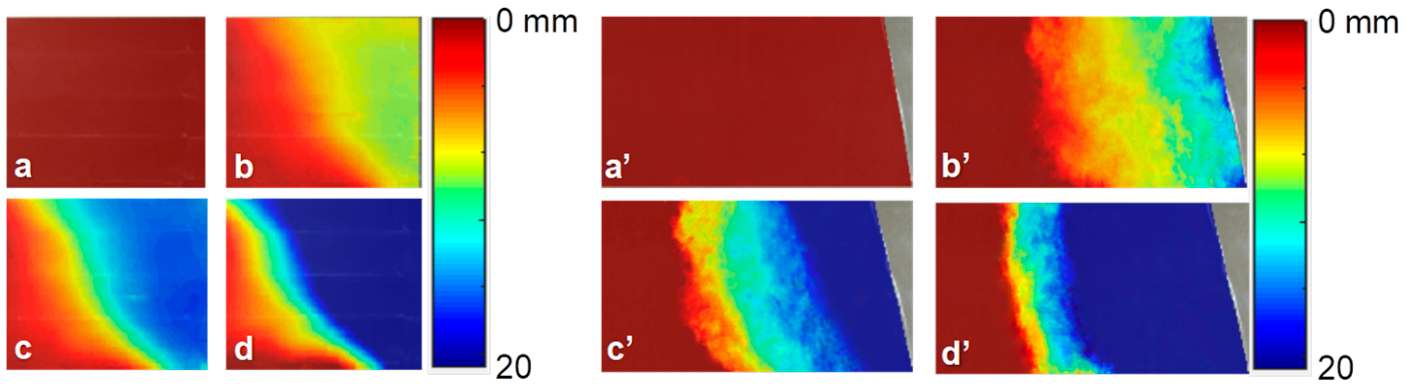
2.5. Results of Physical Model Tests

Through the analysis and calculations using the digital image correlation (DIC) method, displacement cloud diagrams for the passive block during the fault dislocation process in the similar model were obtained. Fault dislocation is initiated by the active block, with the dislocation effects transmitted to the passive block through the fault, causing the mass points within the passive block to exhibit a displacement trend identical to the dislocation direction of the active block. In this case, it results in vertical displacement within the passive block. In the early stages of the test, the vertical displacement gradually propagates from the fault to the interior of the passive block, with the displacement cloud diagram indicating an expanding affected area. As the test progresses, the range of vertical displacement ceases to expand, forming a narrow displacement influence boundary in the displacement cloud diagram. Within this boundary, mass points are subjected to fault dislocation, and the vertical displacement continues to increase. Comparing the displacement cloud diagrams of different types of faults, the range of mass points within the passive block affected by fault dislocation in the strike-slip fault model is smaller than in the reverse fault model (Figure 5).

To clarify the displacement differences in different fault models, the vertical dislocation displacement values at the midpoint of the model (30 cm from the model’s base) are selected. With the fault as the origin of the horizontal coordinates, we draw a line chart based on physical models of the vertical displacement of the passive wall in five stages when the active wall moves 10 mm, 20 mm, 30 mm, 40 mm, and 50 mm (Figure 6, Figure 7 and Figure 8).

The displacement distribution of the three groups of fault physical models all indicate that the vertical displacement exhibits discontinuity at the fault, characterized by a significant abrupt change between the vertical displacements within the passive and active blocks at the fault. The greater the fault dislocation distance, the more pronounced the discontinuity in displacement. Comparing the vertical displacement magnitudes at corresponding points for different types of faults, each corresponding point’s vertical displacement in strike-slip faults is smaller than in reverse faults. This is attributed to the smaller normal stress experienced by the strike-slip fault planes, resulting in reduced displacement within the passive block, thereby illustrating how different external factors can cause varying displacement perturbations within a fault.

The displacement characteristics of reverse faults at different angles indicate that, at the same dislocation distance, the smaller the fault dip angle, the greater the influence of fault dislocation on the passive block. This influence is manifested in two aspects: the range of perturbation and the magnitude of displacement. On one hand, a smaller fault dip angle results in a larger overall volume of the active block, leading to a larger perturbation range during the active block’s uplift, and consequently, an increased range of displacement impact within the passive block. On the other hand, a smaller fault dip angle implies a longer fault length within the model, increasing the internal displacement magnitude of the passive block. This illustrates that under the same type of fault conditions, internal factors are the main determinants of fault displacement perturbations.

3. Displacement Field Inversion

The fault numerical simulation is based on the FLAC^3D v6.0 finite difference numerical simulation software developed by the company ITASCA (Minneapolis, MN, USA). The software’s built-in interface elements can simulate and analyze physical discontinuities such as faults, joints, or the interfaces between artificial structures and natural rocks in geological materials. In the numerical model, the solid elements correspond to the hanging wall and footwall of the physical model, while the interface elements correspond to the faults in the physical model. The dislocation behavior of the interface elements during movement simulates the non-continuity of the faults.

3.1. Numerical Simulation Scheme

The numerical model is established with dimensions corresponding to the physical model, overall measuring 60 cm × 60 cm × 150 cm, with hexahedral mesh elements having a side length of 2 cm. Three sets of numerical models are constructed to correspond to the three sets of physical model tests, specifically, the 60° reverse fault model, the 75° reverse fault model, and the strike-slip fault model. The solid elements in each group of models adopt an elastic constitutive relationship, assigned values based on the mechanical parameters of the similar materials; interface elements utilize a Coulomb shear constitutive model, with internal parameters selected based on the literature [26]. The cohesion and internal friction angle are chosen to be 0.5 to 0.8 times those of the surrounding rock mass, while the normal stiffness and shear stiffness, K_n and K_s, are calculated according to Formula (1):

$$K_n=K_s=\frac{1}{20}\left(\frac{K+\frac{4}{3}G}{\Delta Z_{\min }}\right)$$

(1)

Note: K_n is the normal stiffness, K_s is the shear stiffness, K is the bulk moduli, G is the shear moduli, and ∆Z_min is the smallest width of an adjoining zone in the normal direction.

Stress boundary conditions, fault displacement rate, and the displacement distance of the numerical model are consistent with the physical model. Corresponding stress boundary conditions are applied to different numerical models, and the displacement field of the physical model is fitted in the numerical model.

3.2. Analysis of Sensitive Factors of Fault Displacement

The interface parameters are mainly four parameters: normal stiffness K_n, shear stiffness K_s, cohesion C, and internal friction angle φ. K_n and K_s are equal in the empirical formula; therefore, this section considers three parameters: shear stiffness, cohesion, and internal friction angle. The specific basic parameters of the interface element are shown in

Table 3. Interface element parameter.

Shear Stiffness Ks (GPa)	Cohesion C (MPa)	Internal Friction Angle φ (°)
0.18	15	12

.

To ascertain the impact of different parameters on the numerical simulation results, the method of controlling variables is employed to analyze the effects of three parameters, cohesion, internal friction angle, and shear stiffness, on the displacement of the passive block. Cohesion is varied to 0.5, 1, 2, and 10 times the base parameter; the internal friction angle is set at 13°, 18°, 23°, and 28°; and shear stiffness is varied to 0.5, 1, 2, and 10 times the base parameter for numerical simulations.

The base parameter numerical model of the fault has already exhibited noticeable displacement discontinuity at the fault location. Theoretically, during the model dislocation process, the fault element’s influence on the solid elements occurs on both sides of the fault: the passive block experiences an upward displacement due to the fault friction, while the corresponding active block undergoes a downward displacement due to the same frictional force, resulting in symmetrical effects on both sides of the fault. However, in the model, the active block’s interior is actually affected by the dislocation compression, making its internal displacement not valuable for reference. Therefore, only the displacement within the passive block near the fault is analyzed.

The calculation results for different cohesion fault models are illustrated in Figure 9. All models exhibit the same displacement discontinuity trend, indicating that cohesion does not affect the displacement discontinuity at the fault. Analyzing the vertical displacement difference on both sides of the fault, the maximum displacement difference is 6.22 mm, occurring in the 0.5 times cohesion fault model; the minimum displacement difference is 6.07 mm, occurring in the 10 times cohesion fault model. The overall impact of the fault element’s cohesion on displacement shows that the greater the cohesion, the smaller the vertical displacement difference across the fault.

The calculation results for different internal friction angle fault models are shown in Figure 10. Variations in the internal friction angle do not affect the displacement discontinuity at the fault. Analyzing the vertical displacement difference on both sides of the fault, the maximum displacement difference in the models is 6.29 mm, occurring in the 13° internal friction angle fault model; the minimum displacement difference is 6.06 mm, occurring in the 28° internal friction angle fault model. The impact of the internal friction angle on the vertical displacement across the fault shows that the greater the internal friction angle, the smaller the vertical displacement difference.

The calculation results for different shear stiffness fault models are presented in Figure 11. Changes in shear stiffness also do not affect the displacement discontinuity at the fault. Analyzing the vertical displacement difference on both sides of the fault, the maximum displacement difference in the models is 6.71 mm, occurring in the 0.5 times shear stiffness fault model; the minimum displacement difference is 4.9 mm, occurring in the 10 times shear stiffness fault model. The impact of shear stiffness on the vertical displacement across the fault indicates that the greater the shear stiffness, the smaller the vertical displacement difference.

Overall, the influence of various parameters in the interface element on the displacement difference across the fault shows that the greater the value of the parameter, the smaller the displacement difference across the fault. To identify the dominant factors among the fault element parameters affecting the displacement difference across the fault sides, the coefficient of variation method is used to calculate the weights of each parameter [27], with the specific coefficient of variation calculated according to Formula (2).

$$V_i=\frac{{\sigma }_i}{x_i}$$

(2)

Note: σ_i is the standard deviation of the i-th influencing factor, and x_i is the mean value of the i-th influencing factor.

The weight of each influencing factor is calculated by Formula (3).

$$W_i=\frac{V_i}{{\displaystyle \sum _{i=1}^n{V}_i}}$$

(3)

Note: V_i is the coefficient of variation of the i-th influencing factor, and W_i is the weight of the i-th influencing factor.

Based on the above formulas, the weights of the factors affecting the displacement difference across the fault are calculated, with the weights for cohesion, internal friction angle, and shear stiffness being 1.2, 1.6, and 12.8, respectively. The ranking of the weights is as follows: shear stiffness > internal friction angle > cohesion (Figure 12).

3.3. Numerical Simulation Results of Displacement Field

Based on the aforementioned sensitivity analysis, it has been determined that shear stiffness is the dominant factor affecting the displacement difference across the fault sides. Therefore, in the trial-and-error method, the shear stiffness parameter of the fault element is primarily adjusted to conduct an inversion calculation based on the displacement field observed in the physical model test.

As shown in Figure 13, the numerical simulation results, based on an elastic constitutive numerical model, closely reflect the displacement trends observed in the physical model test. The numerical model mitigates the effects of heterogeneity present in the physical model, exhibiting a linear change in vertical displacement within the area of influence; the displacement impact range is smaller at the base of the model and gradually expands towards the top. The displacement impact range at the bottom of the reverse fault model is noticeably larger than that of the strike-slip fault model.

4. Fault Physical Model Test

By defining the parameters of the interface fault elements in the numerical model, the actual characteristics of fault dislocation can be reflected, allowing for the analysis of fault-induced geostress perturbations. In this section, the numerical model uses boundary conditions relevant to deep reservoir stress to analyze geostress perturbations in the reservoir.

4.1. Single-Fault Analysis

Building on the previous results of fault dislocation numerical simulations, the analysis of geostress perturbations in a single fault model can be conducted by proportionally scaling the numerical model and mechanical parameters based on the similarity ratio. The three faults are F1 (75° reverse fault), F2 (strike-slip fault), and F3 (60° reverse fault), with specific parameters as shown in

Table 4. Numerical simulation parameter.

Element Properties	Modulus of Elasticity (GPa)	Poisson’s Ratio	Normal Stiffness (GPa)	Shear Stiffness (GPa)	Cohesion (MPa)	Internal Friction Angle (°)
Reservoir	24.95	0.18	/	/	/	/
F1	/	/	1.42	1.42	23	21
F2	/	/	0.94	0.94	16	17
F3	/	/	1.57	1.57	19	20

.

The results from all three sets of numerical simulations consistently demonstrate that within the fault dislocation models, both the maximum and minimum principal stresses at the fault decrease, but the extent of reduction varies across different fault models. In the strike-slip fault model, the decrease in stress is smaller, with a reduction of 5.63 MPa in the maximum principal stress and 1.18 MPa in the minimum principal stress at the fault. In contrast, the reverse fault model shows a larger decrease in stress: at the 60° fault, the maximum principal stress decreases by 10.65 MPa and the minimum principal stress by 4.38 MPa; at the 75° fault, the maximum principal stress decreases by 9.96 MPa and the minimum principal stress by 5.02 MPa. In the strike-slip fault model, the overall stress is less perturbed by the fault, attributed to the lower normal stress experienced by the fault plane, resulting in a similarly lower magnitude of stress perturbation during the fault dislocation process (Figure 14).

When comparing the reverse fault models horizontally, the two groups of reverse faults at different angles exhibit the same trend in stress perturbation. The high-angle reverse fault causes a greater perturbation to the maximum principal stress compared to the low-angle reverse fault, but it causes a smaller perturbation to the minimum principal stress than the low-angle reverse fault. The differences in stress perturbation by reverse faults at various angles are primarily concentrated in the area near the fault. In regions far from the fault, the degree of stress perturbation caused by reverse faults at different angles tends to converge.

4.2. Multi-Fault Analysis

In order to further clarify the perturbation of geostress under the combined influence of multiple faults, a multi-fault analysis model is established. The model extends 12 km in the east–west direction (x-axis) and 12 km in the north–south direction (y-axis) and has a thickness (z-axis) of 1 km, covering a total area of 144 km². The numerical model uses hexahedral mesh elements with a side length of 50 m, comprising 434,908 mesh elements and 216,868 nodes (Figure 15).

From left to right, the model includes fault F1 (75° reverse fault), fault F2 (strike-slip fault), and fault F3 (60° reverse fault). In the numerical model, the reservoir matrix elements adopt a linear elastic constitutive model, while the fault interface elements use a Coulomb shear constitutive model, with specific parameters presented in Table 4. The model imposes boundary conditions that restrict lateral displacements on the sides and in all three directions of displacement at the bottom. The numerical model achieves initial equilibrium under the conditions of self-weight and tectonic stress, generating a stress field influenced by fault perturbations.

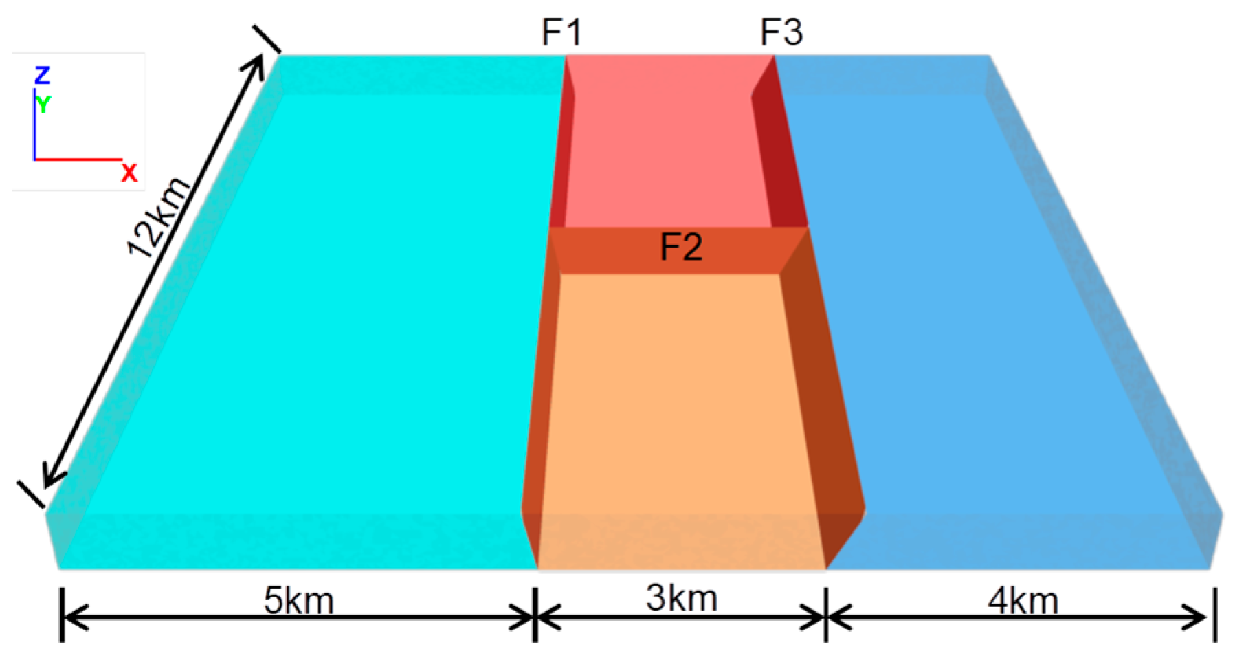
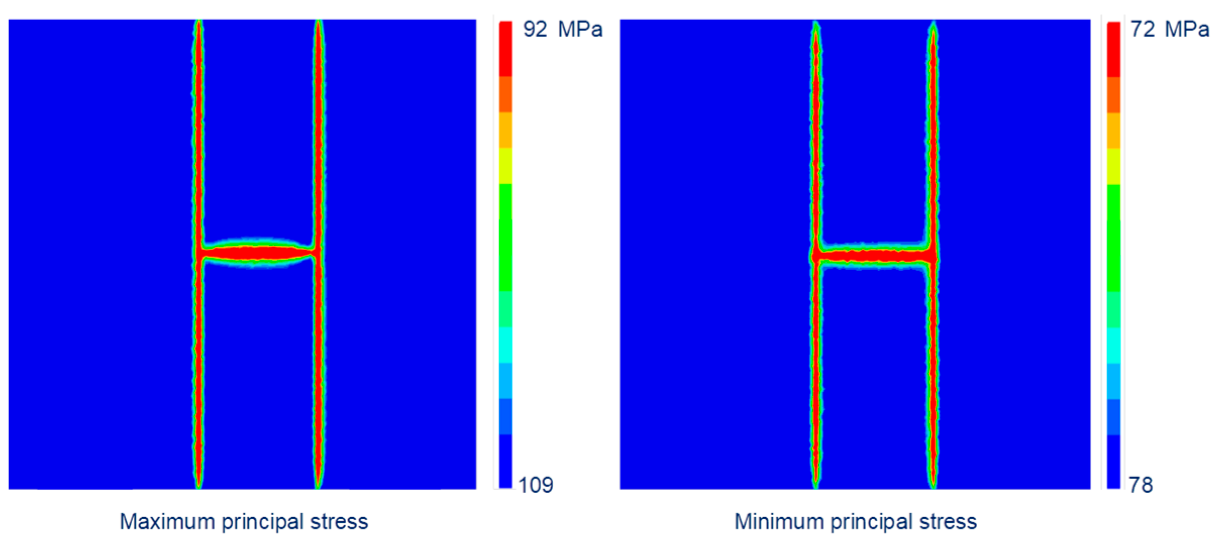
4.3. Simulation Results of Multi-Fault Model

The numerical simulation results of the multi-fault geostress field include the perturbations of the maximum and minimum principal stresses. The perturbation trend is consistent with that of the single fault numerical models, where stress values decrease at the faults, and the degree of stress reduction varies among the faults. The maximum reduction in the maximum principal stress is 16.85 MPa, occurring at the intersection of faults F2 and F3; the greatest decrease in the minimum principal stress is 7.05 MPa, observed at the intersection of F1 and F2. The stress extremities in the numerical model all occur at the intersections of faults, indicating stress concentration at these junctions (Figure 16).

Given that the three faults within the study area differ in scale and characteristics, their impacts on stress perturbations vary as well. The values of the maximum and minimum principal stresses within 800 m of each fault are analyzed, and graphs depicting the relationship between geostress magnitude and distance from the faults are created (Figure 17).

The impact of different types of faults on the maximum principal stress is as follows: F1 (16.85 MPa) > F3 (15.10 MPa) > F2 (11.49 MPa). The impact on the minimum principal stress by different types of faults is F2 (7.05 MPa) > F3 (6.06 MPa) > F1 (4.40 MPa). From the perspective of fault types, reverse faults have a greater impact on the maximum principal stress than strike-slip faults, a conclusion that aligns with the results from the single fault simulations. However, due to the combined effects in the multi-fault scenario, the minimum principal stress impact caused by the strike-slip fault (F2) in the multi-fault model exceeds that caused by the reverse faults, indicating that the minimum principal stress is more susceptible to the interactive influences among faults.

The relationship between the fault’s influence on the geostress value and the fault distance is used to perform function fitting, and the degree of perturbation to the geostress is quantitatively analyzed. Since the stress perturbation of the fault is suitable for exponential fitting, the form of f(x) = ae^bx is used to perform fitting. In the formula, a is the fault stress parameter, b is the distance coefficient, and x is the distance to fault (

Table 5. Fitting parameters.

Fault	a (σH)	b (σH)	a (σh)	b (σh)
F1	16.85	−0.005142	4.40	−0.007573
F2	11.49	−0.004471	7.05	−0.006101
F3	15.01	−0.006211	6.06	−0.007139

).

In the fitting formula, the fault stress parameter a indicates the degree of geostress perturbation caused by the fault. The larger the fault stress parameter, the greater the degree of geostress perturbation at the fault. The distance coefficient b represents the range of fault-induced perturbation; a larger distance coefficient corresponds to a smaller perturbation range. A comprehensive comparison of the fitting parameters for the maximum and minimum principal stresses indicates that in the numerical model, the impact range of all three faults on the minimum principal stress is smaller than their impact range on the maximum principal stress. Using the maximum perturbation stress value of 25% as the boundary stress value for perturbation, the perturbation boundary ranges for different faults are calculated, with the results presented in

Table 6. Boundary distance of stress perturbation amount.

	F1 σH	F1 σh	F2 σH	F2 σh	F3 σH	F3 σh
Distance (m)	269.60	183.06	310.06	194.17	223.20	227.22

.

Within the multi-fault numerical model, under the combined influence of three major faults, the perturbation distance ranges from 183.06 to 310.06 m when considering a 25% stress perturbation as the boundary. The largest range of fault stress perturbation is observed in the influence range of the maximum principal stress for fault F2. Studies by Brudy [28] and Tamagawa [29] indicate that the observed boundaries of stress perturbations in oil and gas development are typically around 200 m. The simulation results for the deep multi-fault development stratum model in this study are consistent with these observed ranges.

5. Conclusions

This article analyzes the effects of fault dislocation on reservoir displacement perturbations by establishing a similar physical model of the fault. The study leverages numerical simulations to ascertain the principal parameters that govern displacement disturbances in reservoirs induced by faults and to invert the stress perturbations associated with fault dislocation displacements. Further, through a geostress analysis model under multi-fault perturbations, the study explores the influence of major internal faults on geostress perturbations, with the main conclusions as follows:

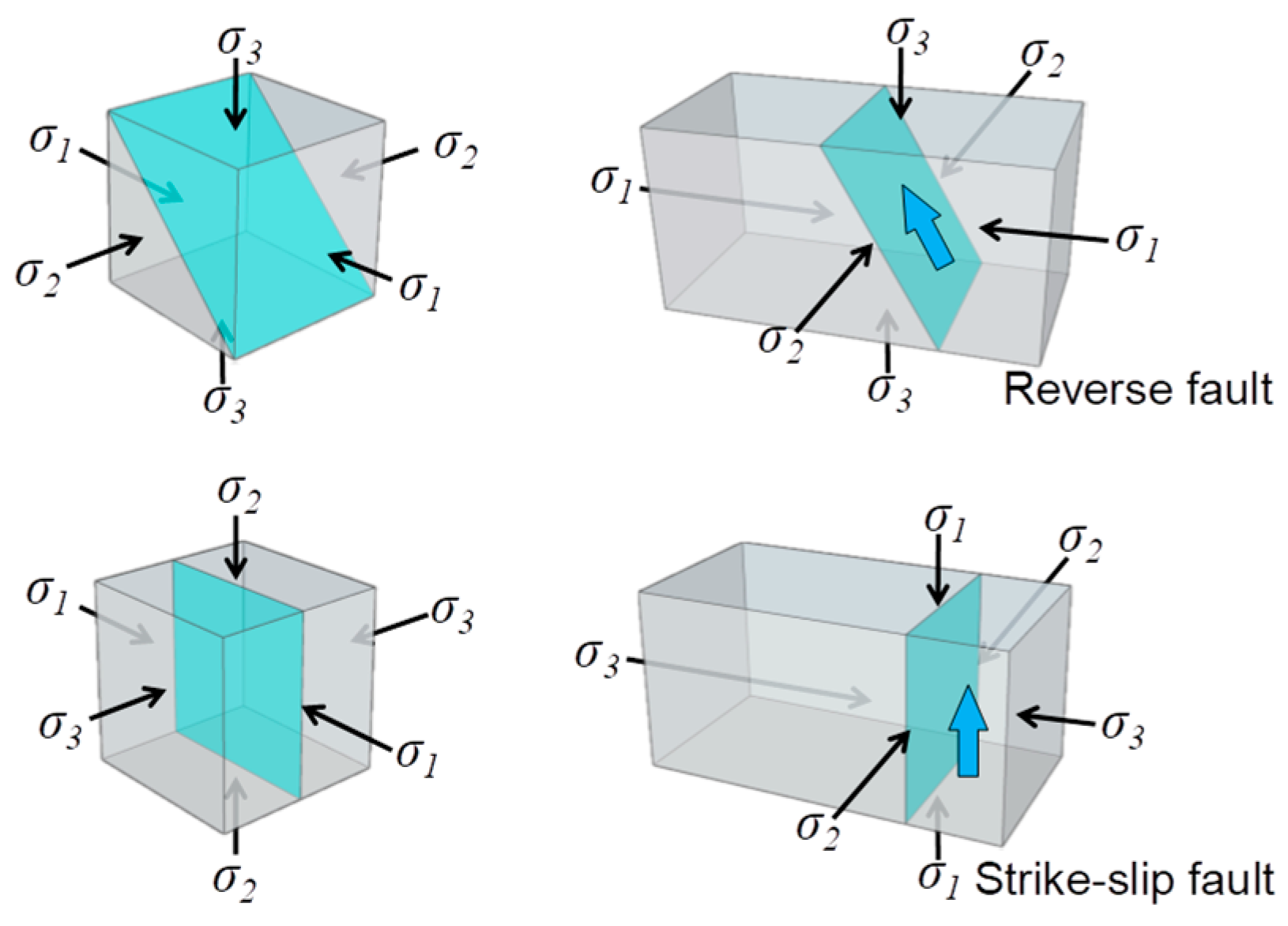
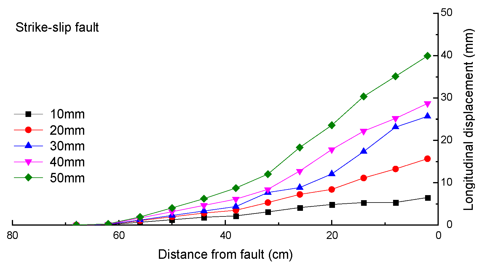
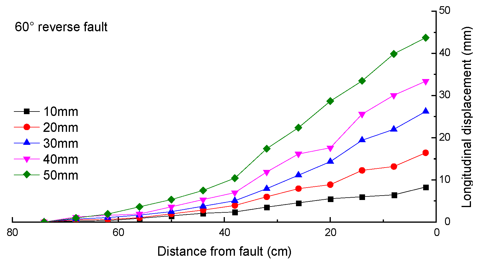
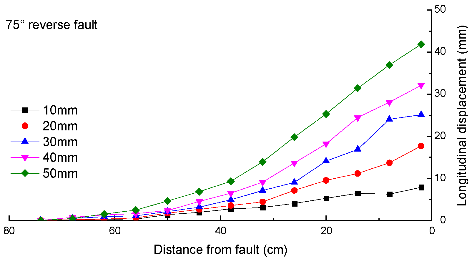
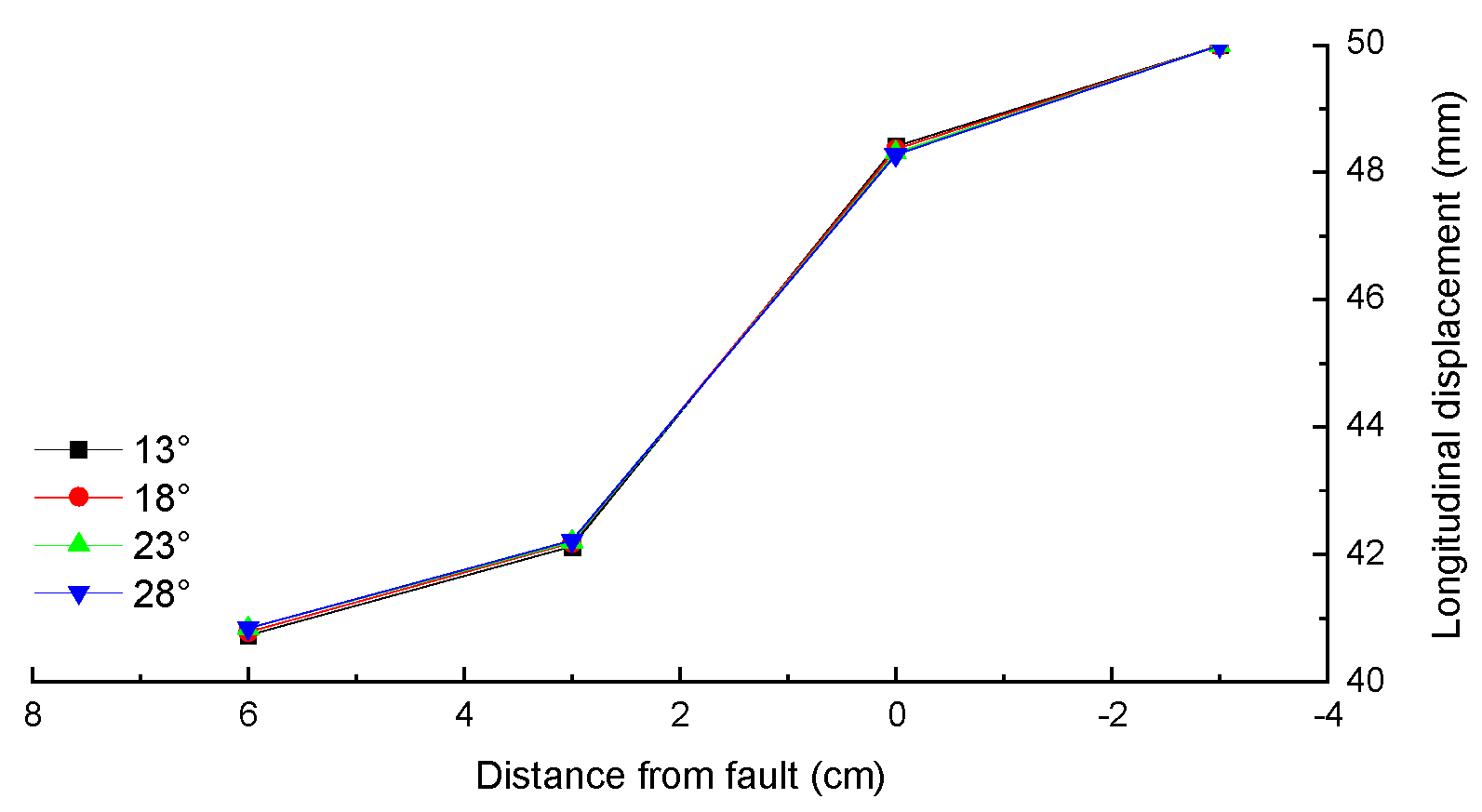
• The impact of faults on reservoirs manifests as the dislocation-induced displacement of the reservoir rock mass. Results from physical model tests indicate that the displacement caused by strike-slip faults is less than that caused by reverse faults; furthermore, low-angle reverse faults induce greater displacement than high-angle reverse faults;
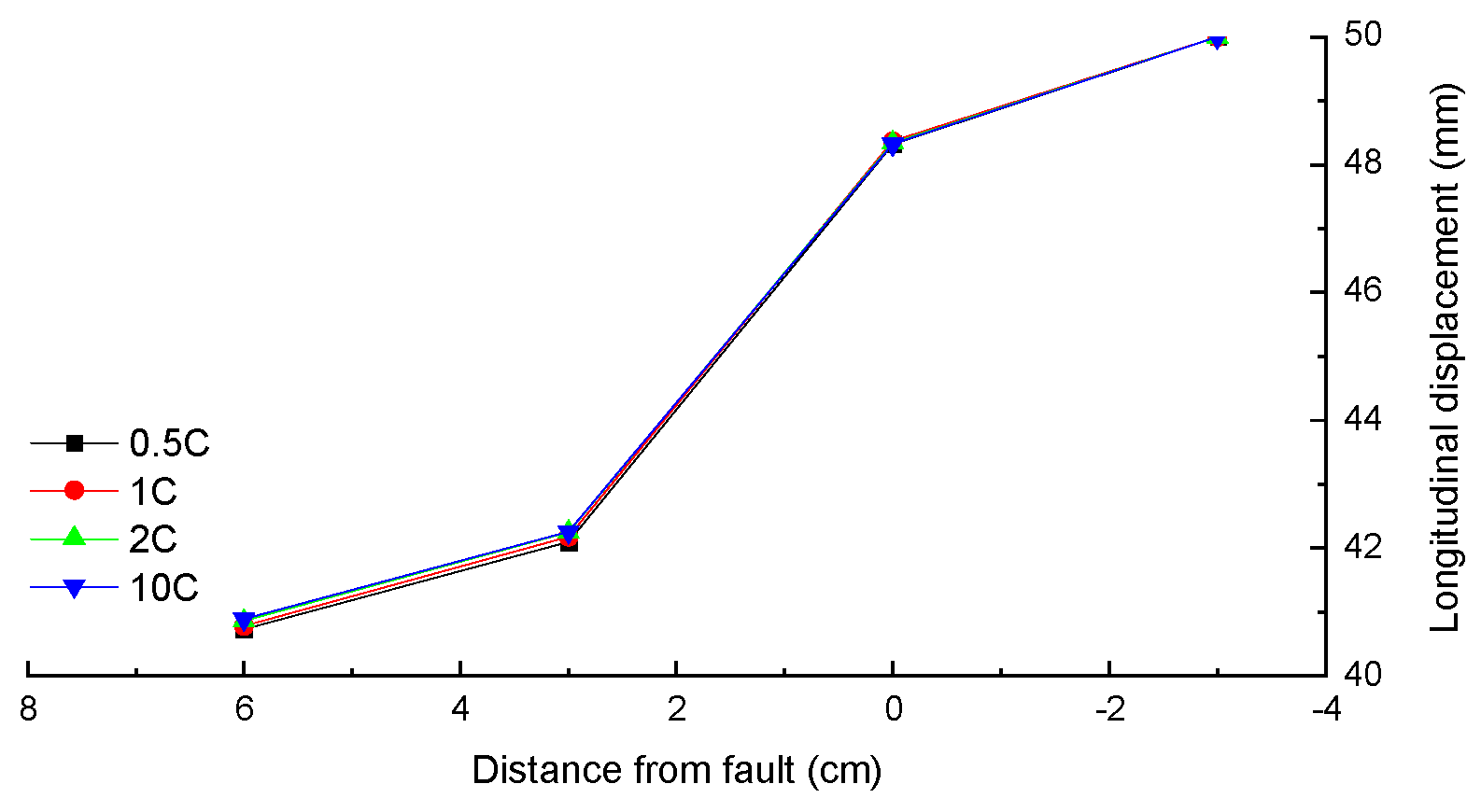
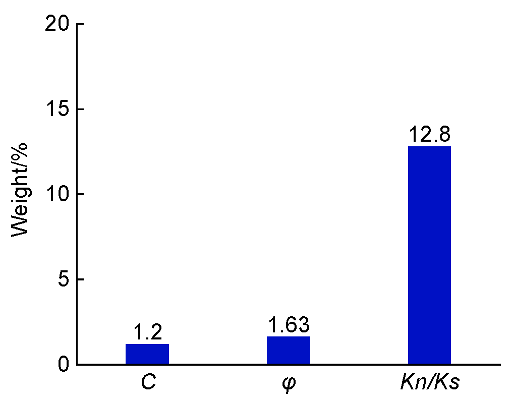
• In the numerical simulation of faults, the cohesion, internal friction angle, and shear stiffness of the fault interface element are all negatively correlated with the displacement difference across the fault sides. Quantitative analysis using the coefficient of variation method to determine the influence weights of these parameters on the displacement difference between the fault sides indicates that shear stiffness is the predominant factor affecting the displacement difference across the fault;
• The outcomes of multi-fault stress field simulations illustrate that faults typically cause a reduction in the horizontal principal stress at the fault locations. However, the extent of geostress reduction and the range of its influence vary among different faults, with the most extensive influence spanning up to 310 m.

References

1. Addis, M. The geology of geomechanics: Petroleum geomechanical engineering in field development planning. Geol. Soc. Spec. Publ. 2017, 458, 7–29. [Google Scholar] [CrossRef]
2. Fjær, E. Geomechanics and geophysics for reservoir management. Rev. Eur. Génie Civ. 2006, 10, 703–730. [Google Scholar] [CrossRef]
3. Yang, S.; Wu, G.; Zhu, Y.; Zhang, Y.; Zhao, X.; Lu, Z.; Zhang, B. Key oil accumulation periods of ultra-deep fault-controlled oil reservoir in northern Tarim Basin, NW China. Pet. Explor. Dev. 2022, 49, 285–299. [Google Scholar] [CrossRef]
4. McClay, K.; Ellis, P. Geometries of extensional fault systems developed in model experiments. Geology 1987, 15, 341–344. [Google Scholar] [CrossRef]
5. Vendeville, B. Mechanisms generating normal fault curvature: A review illustrated by physical models. Geol. Soc. Spec. Publ. 1991, 56, 241–249. [Google Scholar] [CrossRef]
6. Keating, D.P.; Fischer, M.P.; Blau, H. Physical modeling of deformation patterns in monoclines above oblique-slip faults. J. Struct. Geol. 2012, 39, 37–51. [Google Scholar] [CrossRef]
7. Lin, M.; Chung, C.; Jeng, F. Deformation of overburden soil induced by thrust fault slip. Eng. Geol. 2006, 88, 70–89. [Google Scholar] [CrossRef]
8. Bois, T.; Bouissou, S.; Guglielmi, Y. Influence of major inherited faults zones on gravitational slope deformation: A two-dimensional physical modelling of the La Clapière area (Southern French Alps). Earth Planet. Sci. Lett. 2008, 272, 709–719. [Google Scholar] [CrossRef]
9. Mou, Y.; Liang, H.; Su, N.; Guo, W.; Pei, Y. Control of pre-existing faults on transtensional and transpressional fault systems: A perspective from analogue modelling. J. Asian Earth Sci. 2023, 252, 105689. [Google Scholar] [CrossRef]
10. Zhang, X.; Shen, Y.; Qiu, J.; Chang, M.; Zhou, P.; Huang, H.; Zhu, P. Failure and deformation mode for soil and tunnel structure crossing multiple slip surfaces of strike-slip fault in model test. Soil. Dyn. Earthq. Eng. 2024, 179, 108541. [Google Scholar] [CrossRef]
11. Bonini, L.; Fracassi, U.; Bertone, N.; Maesano, F.E.; Valensise, G.; Basili, R. How do inherited dip-slip faults affect the development of new extensional faults? Insights from wet clay analog models. J. Struct. Geol. 2023, 169, 104836. [Google Scholar] [CrossRef]
12. Martin, C.D.; Chandler, N.A. Stress heterogeneity and geological structures. Int. J. Rock Mech. Min. Sci. Geomech. Abstr. 1993, 30, 993–999. [Google Scholar] [CrossRef]
13. Zoback, M.D.; Zoback, M.L.; Mount, V.S.; Suppe, J.; Eaton, J.P.; Healy, J.H.; Oppenheimer, D.; Reasenberg, P.; Jones, L.; Raleigh, C.B. New evidence on the state of stress of the San Andreas fault system. Science 1987, 238, 1105–1111. [Google Scholar] [CrossRef] [PubMed]
14. Tingay, M.; Muller, B.; Reinecker, J.; Heidbach, O. State and origin of the present-day stress field in sedimentary basins: New results from the World Stress Map Project. In Proceedings of the Golden Rocks 2006, the 41st U.S. Symposium on Rock Mechanics (USRMS), Golden, CO, USA, 17–21 June 2006; ARMA: Alexandria, VA, USA,, 2006; p. ARMA-06-1049. [Google Scholar]
15. Wang, K.; Dai, J.; Liu, H.; Li, Q.; Zhao, L. Characteristic of current in-situ stress field in Keshen gas field, Tarim Basin. Zhongnan Daxue Xuebao (Ziran Kexue Ban)/J. Cent. South Univ. (Sci. Technol.) 2015, 46, 941–951. [Google Scholar]
16. Congro, M.; Zanatta, A.S.; Nunes, K.; Quevedo, R.; Carvalho, B.R.; Roehl, D. Determination of fault damage zones in sandstone rocks using numerical models and statistical analyses. Geomech. Energy Environ. 2023, 36, 100495. [Google Scholar] [CrossRef]
17. Zhang, J.; Zhang, Z.; Wang, B.; Deng, S. Development pattern and prediction of induced fractures from strike-slip faults in Shunnan area, Tarim Basin. Oil Gas Geol. 2018, 39, 955–963+1055. [Google Scholar]
18. Zhang, B.; Hu, X.; Wang, Y.; Hu, Y.; Chen, W. In situ stress inversion and fracture characteristics around local fault in deep heterogeneous strata. Pet. Sci. Technol. 2024, 42, 448–469. [Google Scholar] [CrossRef]
19. Jiao, Z.; Wang, L.; Zhang, M.; Wang, J. Numerical simulation of mining-induced stress evolution and fault slip behavior in deep mining. Adv. Mater. Sci. Eng. 2021, 2021, 1–14. [Google Scholar] [CrossRef]
20. Chen, B.; Ren, Q.; Wang, F.; Zhao, Y.; Liu, C. Inversion analysis of in-situ stress field in tunnel fault zone considering high geothermal. Geotech. Geol. Eng. 2021, 39, 5007–5019. [Google Scholar] [CrossRef]
21. Yoon, J.S.; Zang, A.; Stephansson, O. Numerical investigation on optimized stimulation of intact and naturally fractured deep geothermal reservoirs using hydro-mechanical coupled discrete particles joints model. Geothermics 2014, 52, 165–184. [Google Scholar] [CrossRef]
22. Sun, L.; Zhu, Y. The research progress on numerical analysis method of initial geostress. Seismol. Geomagn. Obs. Res. 2008, 29, 14–21. [Google Scholar]
23. Cappa, F.; Rutqvist, J. Impact of CO2 geological sequestration on the nucleation of earthquakes. Geophys. Res. Lett. 2011, L17313, 1–6. [Google Scholar] [CrossRef]
24. Shen, H.; Cheng, Y.; Zhao, Y.; Zhang, J.; Xia, Y. Study on influence of faults on geostress by measurement data and numerical simulation. Yanshilixue Yu Gongcheng Xuebao/Chin. J. Rock. Mech. Eng. 2008, 27, 3985–3990. [Google Scholar]
25. Zhu, A.; Zhang, D.; Jiang, C. Numerical simulation of the segmentation of the stress state of the Anninghe-Zemuhe-Xiaojiang faults. Sci. China Earth Sci. 2016, 59, 384–396. [Google Scholar] [CrossRef]
26. Cai, S. Research and Application of Contact Surface Method and Weakening Method in FLAC3D Fault Simulation. Master’s Thesis, China University of Mining and Technology, Xuzhou, China, 2016. [Google Scholar]
27. Yu, Y. Evaluation of weighting methods in multi-index comprehensive evaluation. Stat. Decis. 2006, 13, 17–19. [Google Scholar]
28. Brudy, M.; Zoback, M.; Fuchs, K.; Rummel, F.; Baumgärtner, J. Estimation of the complete stress tensor to 8 km depth in the KTB scientific drill holes: Implications for crustal strength. J. Geophys. Res. Solid. Earth 1997, 102, 18453–18475. [Google Scholar] [CrossRef]
29. Tamagawa, T.; Pollard, D.D. Fracture permeability created by perturbed stress fields around active faults in a fractured basement reservoir. AAPG Bull. 2008, 92, 743–764. [Google Scholar] [CrossRef]
Figure 1. Fault dislocation simulation test platform under triaxial stress.
Processes 12 01240 g001
Figure 2. Structure of fault physical model.
Processes 12 01240 g002
Figure 3. Stress boundary conditions.
Processes 12 01240 g003
Figure 4. DIC analysis area. (a) Strike-slip fault; (b) reverse fault.
Processes 12 01240 g004
Figure 5. Displacement field of fault dislocation model: (a,a’) 0 cm displacement of active block; (b,b’) 20 cm displacement of active block; (c,c’) 40 cm displacement of active block; (d,d’) 50 cm displacement of active block.
Processes 12 01240 g005
Figure 6. Vertical displacement of strike-slip fault.
Processes 12 01240 g006
Figure 7. Vertical displacement of 60° reverse fault.
Processes 12 01240 g007
Figure 8. Vertical displacement of 75° reverse fault.
Processes 12 01240 g008
Figure 9. Effect of cohesion on vertical displacement.
Processes 12 01240 g009
Figure 10. Effect of internal friction angle on vertical displacement.
Processes 12 01240 g010
Figure 11. Effect of shear stiffness on vertical displacement.
Processes 12 01240 g011
Figure 12. Weight of factors affecting vertical displacement.
Processes 12 01240 g012
Figure 13. Displacement fields of physical and numerical models. (a) Strike-slip fault; (b) reverse fault.
Processes 12 01240 g013
Figure 14. Relationship between principal stress and fault distance.
Processes 12 01240 g014
Figure 15. Multi-fault numerical model.
Processes 12 01240 g015
Figure 16. Multi-fault principal stress simulation results.
Processes 12 01240 g016
Figure 17. Relationship between multi-fault principal stress and fault distance.
Processes 12 01240 g017