Identification Method of Stuck Pipe Based on Data Augmentation and ATT-LSTM

Abstract

Stuck pipe refers to the accidental phenomenon whereby drilling tools are stuck in a well during the drilling process and cannot move freely due to various reasons. As a result, the stuck pipe can consume a lot of manpower and material resources. With the development of artificial intelligence, the intelligent prediction and identification of stuck pipe risk has gradually advanced. However, there are usually only a few stuck samples, so the intelligent model is not sufficient to excavate the stuck feature law, and then the model overfitting phenomenon occurs. Regarding the above issue, this paper proposed a limited incident dataset method based on data augmentation. Firstly, in terms of data processing, by applying percentage scaling and random dithering to the original data and combining it with GAN to generate new data, the training dataset was effectively extended, solving the problem of insufficient sample size. Then, in the selection and training of the intelligent model, an LSTM neural network model with an attention mechanism (ATT-LSTM) is introduced. By applying the attention mechanism in each time step, the model can dynamically adjust the degree of attention to different parts of the sequence and better capture the key information in the data, which improve the accuracy of the recognition and the generalization ability of the model. By testing the trained model on field data, the test results show that the method achieves more significant performance improvement on the stuck pipe recognition task, and the prediction accuracy of the intelligent model increases by 21.31% after data enhancement.

1. Introduction

The phenomenon in the drilling process where the drilling tools become stuck in the wellbore due to various reasons and cannot move freely is called a stuck pipe incident. According to statistics on drilling situations in oilfields in Western China, stuck pipe incidents account for 40% to 50% of all drilling accidents, and the financial costs caused by stuck pipe incidents represent more than half of the non-production costs [1]. Although a considerable amount of research has been conducted on the treatment of stuck pipe incidents both domestically and internationally, and many advanced and effective treatment methods have been proposed, in actual drilling operations, on-site personnel mainly rely on experience to provide qualitative operations to prevent stuck pipe incidents. This leads to the blindness of drilling operations and the inability to predict stuck pipe incidents on time, resulting in the occurrence of stuck pipe incidents [2]. Machine learning, as a branch of artificial intelligence, aims to study how to enable computer systems to acquire knowledge from data through learning and make autonomous decisions and predictions based on this knowledge. Its core principle lies in building models using training data and then using these models for prediction or decision-making. When addressing classification problems, machine learning builds classification models by learning from known data, enabling the classification of new data [3]. Therefore, identifying stuck pipe incidents, which fundamentally belongs to a classification task, can also be performed using machine learning algorithms.

In recent years, the application of artificial intelligence in engineering has attracted significant attention. Researchers have conducted extensive studies on the intelligent prediction of stuck pipe incidents. Many scholars have used artificial neural networks as standalone tools, collecting data from multiple oilfield sites and training neural networks with different input parameters and data sizes to achieve intelligent prediction of stuck pipe incidents. Research results have shown that neural networks can predict stuck pipe incidents with varying degrees of accuracy [4,5]. Naraghi et al. [6] utilized fuzzy logic and active learning for stuck pipe prediction, identifying that rotary table speed and gel strength have the most significant impact on stuck pipe incidents. Salminen et al. [7] studied automatic real-time modeling and data analysis methods for predicting stuck pipe risks, and the model predictions are more prominent. Mora et al. [8] used variance analysis for feature extraction, selecting feature parameters related to stuck pipe incidents, and established a stuck pipe classification model using the random forest algorithm; the model also has good prediction accuracy. Liu Guangxing et al. [9] combined autoregressive moving average models with neural network modeling to successfully predict stuck pipe incidents. Liu Dongdong et al. [10] developed a stuck pipe causation analysis method based on fault tree analysis, achieving high accuracy in stuck pipe prediction when the accident causes are known. Wu Jun et al. [11] established a stuck pipe prediction model using support vector machine algorithms, with a prediction accuracy of 98.08%. Li Tong et al. [12] used drilling time, speed, torque, pump pressure, and drill pressure as neural network input parameters, optimizing them using the PSO algorithm and significantly improving the prediction accuracy of the stuck pipe model. Reddy K M et al. [13] proposed a new method for detecting stuck events in drilling using autoencoder in deep learning by constructing an autoencoder model on a recurrent neural network to model normal drilling activities and identify anomalous activities as stuck events. Experimental results show promising performance in detecting stuck signs in actual data from multiple drilling sources. Additionally, reconstruction analysis on individual drilling parameters was conducted to explain the trained model’s predictions. Asad E et al. [14] detected formation issues by constructing a risk prediction window, helping to take corrective actions on site in advance. Testing on historical datasets showed successful detection within an average duration of 120 min before the incidents occurred.

When processing stuck pipe data, it is often found that the sample size of stuck pipe data is limited and generally insufficient to support the training of intelligent models and therefore the use of small sample learning methods are considered for processing the data. In cases where the number of data samples is limited, some data augmentation methods can be employed to increase the sample data volume.

Mechanical stuck pipe refers to a situation in drilling operations where the drill string or drilling tools become trapped in the wellbore due to some mechanical reasons, making it unable to move freely up and down or rotate. Common types of mechanical stuck pipe include keyseat stuck pipe and differential sticking. In order to improve the performance of intelligent recognition methods for mechanical stuck pipe incidents, this paper proposes a stuck pipe risk data generation method using percentage scaling, random perturbation, and combining GANs. Additionally, to more effectively explore limited stuck pipe risk data, an LSTM stuck pipe intelligent identification model with an attention mechanism is established. By combining these two methods, even with very limited stuck pipe risk data, the model can achieve high recognition accuracy [15]. This enables an accurate prediction of on-site stuck pipe incidents.

2. Methodology

2.1. Brief Process

The limited original stuck pipe data are first cleaned using methods such as data denoising and data normalization. The cleaned data are then augmented and extended through techniques like percentage scaling, random perturbation, and data generation using GANs. The appropriate sliding window size is determined through grid search, and the augmented data are transformed into sequential data required by the intelligent model using the sliding window approach. 70% of the data are used for training, while 30% are used for testing. The data are then fed into an LSTM neural network model with an attention mechanism for training. Finally, the trained model is tested with actual data, and the results are analyzed, as shown in Figure 1. The specific steps for each part are described in detail in the corresponding sections.

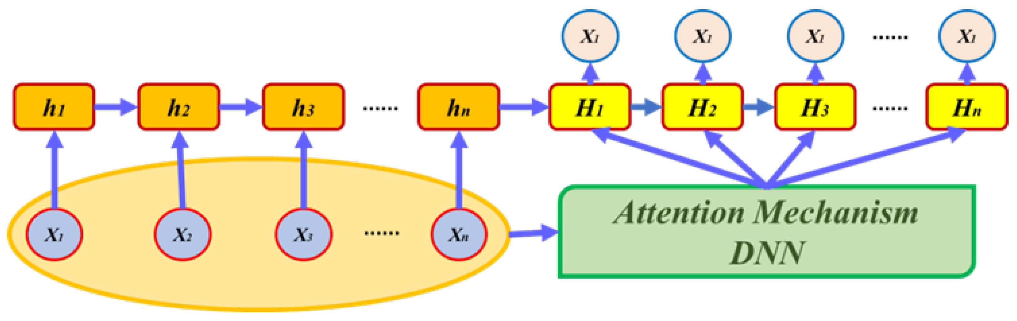
2.2. Long Short-Term Memory (LSTM) and Attention Mechanism

The data used for stuck pipe condition recognition and detection are time series data, exhibiting temporal characteristics. Traditional recurrent neural networks (RNNs) can handle one-dimensional time series data, but their ability to learn long-term dependencies is limited due to issues such as vanishing or exploding gradients. Compared to the traditional recurrent neural network (RNN), the unitary state $Q_{\mathrm{t}}$ is introduced in the LSTM neural network for preserving long-term memory at time step $t$. In this process, the forgetting gate $A_{\mathrm{t}}$, the input gate $S_{\mathrm{t}}$, and the output gate $F_{\mathrm{t}}$ play a key role. Among them, the input gate $S_{\mathrm{t}}$ and the forgetting gate $A_{\mathrm{t}}$ together determine what new information should be added to the current long-term memory unit state $Q_{\mathrm{t}}$. In this process, the past output value $P_{\mathrm{t}-1}$ and cell state $Q_{\mathrm{t}-1}$ represent the output value and cell state of the LSTM at time step $t-1$, respectively. The input value $x_{\mathrm{t}}$ and output value $P_{\mathrm{t}}$ at the current moment denote the input and output of the LSTM at time step $t$, respectively. In the gating mechanism of LSTM, the sigmoid function O is used to generate the gating signals with output values ranging from [0, 1], while the hyperbolic tangent function tanh is used to generate the state values with output values ranging from [−1, 1]. M1, M2, M3, and M4 denote the weights of oblivion gates, input gates, cell state update, and output gate weights, which play a role in regulating the importance of different parts of the LSTM network. The unit state, oblivion gate, input gate, and output gate in the LSTM together form a complex gating mechanism. Through the control of these gating units, the LSTM network can better deal with long sequential data, maintain long-term memory, and dynamically update the internal state according to the current input, thus improving the learning and prediction ability of the network [16]. In summary, the memory blocks, memory cells, input gates, output gates, and forget gates in the LSTM structure work together to efficiently process sequential data, maintain long-term memory, enhance the network’s learning ability, and improve prediction accuracy. This paper establishes a stuck pipe risk identification model based on LSTM neural networks with attention mechanisms, used for stuck pipe incident identification and prediction [17], as shown in Figure 2.

The LSTM neural network with attention mechanism is a deep learning model that combines long short-term memory (LSTM) and attention mechanism. Traditional RNNs and LSTMs face challenges in capturing long-term dependencies and processing the entire sequence globally when dealing with long sequential data. In contrast, the LSTM with an attention mechanism can assign different attention weights to different parts of the input sequence, effectively capturing important information within the sequence.

The principle involves calculating attention scores at each time step by using the current hidden state and historical hidden states to determine the relevance between the current time step and historical time steps, thereby deciding the level of focus on the current input. The attention scores are normalized using the Softmax function to obtain attention weights for each time step. These weights are then used to compute a weighted sum, resulting in a context vector that is combined with the input at the current time step to generate a new representation. This approach allows the model to assign varying levels of importance to different parts of the input, enabling better capture of key information within the sequence. This addresses the challenge of handling long-term dependencies faced by traditional LSTMs, while also enhancing the interpretability and performance of the model, as shown in Figure 3.

2.3. Few-Shot Learning and Data Augmentation

Few-shot learning (FSL) is a machine learning method that specifically addresses the problem of constructing effective models in the presence of scarce data. In traditional supervised learning, a large amount of labeled data are usually required to train the model to obtain good generalization performance. However, obtaining large amounts of labeled data is difficult or even infeasible in many real-world scenarios, such as medical diagnosis, natural language processing, and the field of stuck pipe risk identification, which is the main focus of this paper. Small sample learning methods usually include meta-learning, transfer learning, generative adversarial networks (GANs), similarity-based methods, and so on. One of the data processing methods used in this paper includes GAN. This is a model that generates realistic data and can be used to generate additional training samples to help the model learn more information about the data distribution, improving the prediction accuracy and generalization of the model.

Data augmentation is a commonly used data preprocessing technique to generate more training samples by applying various transformations and expansions to the original data. The main purpose of data augmentation is to increase the diversity of the data and improve the generalization ability and robustness of the model while reducing the risk of overfitting [18]. Commonly used data enhancement methods include rotation, flipping, scaling, panning, cropping, adding noise, color transformation, elastic transformation, mixing samples, etc. Data enhancement techniques can choose appropriate transformations according to the characteristics of specific tasks and datasets, thus effectively improving the performance and generalization ability of the model. In the field of deep learning, data enhancement has become one of the indispensable and important techniques when training models [19].

In this paper, to increase the amount of data in the stuck pipe samples, a data enhancement method based on percentage scaling, random jitter and generative adversarial networks (GANs) is proposed. The original data sequence is multiplied by a random scalar and then a random deviation is added to generate a new data sequence with the same overall change trend. The formula for percentage scaling and random jitter is given by Formula (1):

$$a_i=x_i{w}_i+b_i$$

(1)

where $x_i$ and $a_i$ represent the $x$-th original data value and augmented data value, and $w_i$ and $b_i$ denote the corresponding random variables and biases.

The above processed data samples are fed into the GAN, where the generator (G) receives random noise input and generates new synthetic data samples, while the discriminator (D) also receives the same random noise input and generates new synthetic data samples. The discriminator (D) then receives real data samples along with the synthetic data samples generated by the generator and undergoes binary classification training. During adversarial training, the generator learns to produce realistic synthetic data, while the discriminator learns to distinguish between real and synthetic samples, i.e., to differentiate between true and false samples, as shown in Figure 4.

Through this adversarial training process, the generator and discriminator engage in competitive learning and optimization, improving the realism of the synthetic data generated by the generator and enhancing the discriminator’s ability to differentiate between real and fake samples. This competitive learning dynamic drives the generator to produce increasingly realistic synthetic data and helps the discriminator to continually improve its ability to discriminate between real and synthetic data. As shown in Equation (2), G is the generator function that generates synthetic data from a random noise vector z, i.e., G(z). D is the discriminator function that outputs the probability that a given data sample x is real, i.e., D(x). xp_data(x) denotes that x is sampled from the true data distribution p_data. zp(z) denotes that z is sampled from a prior distribution p_z (e.g., a standard normal distribution).

$$mi{n}_{\mathrm{G}}ma{x}_{\mathrm{D}}DV\left(D,G\right)=E_{x\sim p_{\mathrm{dt}}\left(x\right)}\left[\log D\left(x\right)\right]+E_{z\sim p_z\left(z\right)}\left[\log \left(1-D\left(G\left(z\right)\right)\right)\right]$$

(2)

Repeat the above steps to optimize the parameters of the generator and the discriminator until a satisfactory generation effect is achieved. Through the above-mentioned methods, the dataset has been expanded from the original 150 million records to 600 million records. The generated synthetic data can be used to train the target model together with the original data to improve the generalization ability of the model. However, GAN technology still faces several limitations, including unstable training, mode collapse, mode dropping, the requirement of substantial data and computational resources, as well as challenges in pattern recognition. These obstacles affect the performance and stability of GANs, necessitating further research and improvement to address them.

2.4. Method Limitations

These methods still have some limitations. Firstly, the data augmentation method used in this study is relatively simple, and employing more advanced and comprehensive data augmentation methods could further enhance the prediction performance of the intelligent model. Secondly, models with attention mechanisms are more complex and difficult to interpret, i.e., “black box” models. This means it is difficult to understand how the model makes decisions. There may also be issues with high computational intensity affecting response times.

3. Data Processing

3.1. Data Sources

The experimental data come from the actual monitoring data of ten wells in the field. The quantity and quality of the training data determine the efficiency of the machine learning method. Noise, missing values, or outliers usually exist in the field data due to sensor failures or environmental disturbances, etc. If the collected field data are directly used for model training, the model fitting process will be slow and the recognition performance will be degraded. Therefore, preprocessing the field data is a necessary step for training the neural network model, including handling missing values, outliers, data denoising, data normalization, and so on.

3.2. Parameter Selection

The mutual information method is used for parameter selection. The mutual information method is a feature selection method for assessing the correlation between features and target variables. It is based on the concept of information theory and measures the degree of information sharing between features and target variables to determine the importance of features to the target variables. Firstly, for each feature Xi and target variable Y, the mutual information value between them is calculated. Then, the features are ranked according to the mutual information value, and the features with high mutual information value are usually selected as important features. The top k features are selected as the final feature set based on the sorting result, or a threshold can be set to filter the features, as shown in Equation (3). I(X; Y) is the mutual information between two random variables X and Y. p(x) is the probability distribution of X. p(x,y) is the joint probability distribution of X and Y.

$$I\left(X;Y\right)=\left(-\sum p\left(x\right)\log p\left(x\right)\right)+\left(-\sum p\left(y\right)\log p\left(y\right)\right)+\sum \sum p\left(x,y\right)\log p\left(x,y\right)$$

(3)

The mutual information scores of different features in the field data were calculated by the mutual information method, as shown in Figure 5, and then combined with the actual experience in the field, for example, the parameters of riser pressure, torque, and drilling pressure have a large impact on stuck pipe, while the parameters of inlet and outlet flow rate and total pool volume have a very small impact on stuck pipe. To sum up, the eight characteristic parameters of riser pressure, big hook height, drill position, rotary speed, torque, drilling pressure, big hook load, and well depth are selected. The statistical information of each parameter is shown in

Table 1. Statistics of partial parameter information.

Factor	Max	Min	Mean	Standard Deviation
Bit Depth (m)	4990.14	3632.43	4475.33	415.22
Hook Load (kN)	2142.15	113.3	984.39	708.79
Drilling Weight (MPa)	1149.35	0	0.005	14.32
Hook Height (m)	36.89	6.85	24.54	10.26
Rotary Speed (rpm)	36.43	0	4.27	10.98
Torque (N·m)	33.46	0	1.41	2.93
Stand Pipe Pressure (MPa)	25.74	0	3.44	7.94
Inlet Flow (m3/s)	52.53	0	44.34	14.67
Outlet Flow (m3/s)	82.3	0	62.96	24.50
Casing Pressure (MPa)	0.36	0	0.19	0.09
Total Pump Strokes (L/s)	32,374.74	14,137.29	22,947.51	4574.47
Total Mud Volume (m3)	118.24	106.03	110.78	3.33

. The data as a whole present the characteristics of high dynamics, non-periodicity, and large span.

3.3. Data Augmentation

The data are generated using the data enhancement method proposed in this paper. Figure 6 shows the model input parameters before and after data enhancement, including parameters such as stand pipe pressure, hook height, bit depth, rotary speed, torque, drilling weight, hook load, and depth. The blue curve represents the original data for each parameter, the red curve represents the data scaled by percentage, the green curve represents the data scaled by percentage with random jitter, and the purple curve represents the data generated by the GAN. It can be seen that the changing trend before and after data augmentation is almost the same and the original sticking characteristics are preserved to the greatest extent. The augmented dataset will be used for training and testing an LSTM neural network model with an attention mechanism.

3.4. Data Normalization

To address issues such as long training times or overfitting, the Min–Max method is employed. The Min–Max normalization technique is a commonly used data normalization method that scales data to a specific range. This method scales the original data to lie between specified minimum and maximum values through linear transformation, typically within the range of [0, 1]. The formula for the Min–Max normalization method is shown in Equation (4):

$$x_{scale}=\frac{x-x_{\min }}{x_{\max }-x_{\min }}$$

(4)

Wherein, x represents the original data, $x_{\min }$ is the minimum value in the original data, $x_{\max }$ is the maximum value in the original data, and $x_{\mathrm{scale}}$ is the normalized data.

The Min–Max normalization method preserves the distribution shape of the original data while scaling it to a fixed range, aiding in accelerating model convergence speed and enhancing model stability and accuracy. This normalization method is commonly used in machine learning algorithms such as neural networks and support vector machines to improve model performance.

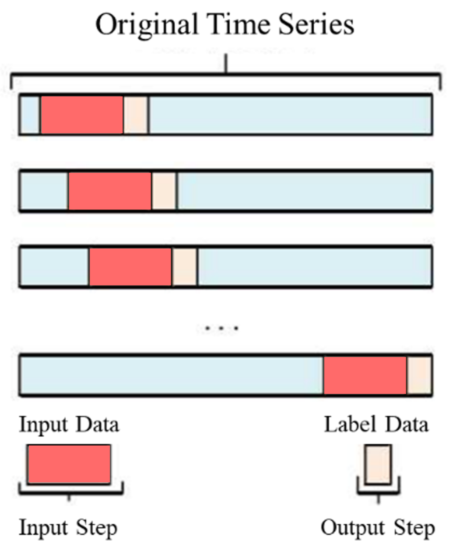
3.5. Dataset Construction

To evaluate the model performance during the training process, the annotated dataset is divided into two subsets: a training set and a test set. Following the current practice, 70% of the entire dataset is used for training, while the remaining 30% is used for testing. Sample data are constructed from the dataset using a sliding time window, where past data points are used to predict the future trend of drilling label changes.

In this experiment, a grid search is conducted to explore the impact of the sliding window size on the model’s prediction accuracy. The optimal sliding window size of 50 was chosen through a grid search, with a movement of one data interval each time, to form the training and testing sample sets. The overall processing procedure is illustrated in Figure 7. In this approach, the original time series data (represented by the blue segments) is partitioned into a sequential series of contiguous, fixed-length sliding windows. Each window encapsulates a set of historical data points, which serve as inputs (indicated in red) to the model. Subsequently, one or more data points following each sliding window are designated as the target variable, referred to as the “label data”. The sliding window progresses forward, advancing by a single unit of time, herein defined as the “output step” (highlighted in yellow), with each movement. This progression incorporates fresh historical data into the succeeding window and refreshes the corresponding output data accordingly. This procedure iterates until the complete time series is traversed, thereby generating a plethora of instances for both training and validation sets.

4. Model Construction

LSTM, ATT-LSTM, and other machine learning models were compared to obtain the optimal performance of the stuck drill prediction model. The performance indexes included mean squared error, absolute error, and accuracy.

In the neural network model, an architecture with a three-layer long short-term memory (LSTM) structure was chosen. The model consists of an input layer, a hidden layer and an output layer. The input layer is used to receive raw data, the LSTM units in the hidden layer are responsible for learning patterns and relationships in the data, and the output layer generates the final prediction results. After cross-validation, data size analysis and a balanced consideration of model performance and generalization capability, it was determined that each layer of the LSTM neural network model contains 128 neurons. The setting of 128 neurons provides sufficient parameter capacity so that the model is able to adequately learn the complex relationships and patterns in the data while avoiding the problem of overfitting.

At the same time, the ATT-LSTM model was constructed with all the same parameters as described above, but the attention mechanism at each time step was further introduced. The model’s attention to different parts of the input sequence can be dynamically adjusted, thus enabling the model to better capture important information and patterns in the sequence data. In this way, ATT-LSTM can more accurately predict the future trends of time series data. During the training process, the Adam optimization algorithm is chosen to minimize the loss function, which is an optimization algorithm that combines momentum and adaptive learning rate to improve the convergence speed and performance of the model. The Adam algorithm can automatically adjust the learning rate during the training process, which makes it possible to better adapt to the characteristics of the data during different parameter updating steps, and thus to converge to the optimal solution more quickly. To avoid the overfitting phenomenon, L2 regularization is used. L2 regularization penalizes the model complexity by adding the sum of squares of the weights to the loss function, thus preventing the model from overfitting the training data. The regularization parameter is introduced to control the extent to which the regularization term affects the loss function and is set to 0.001 through a grid search and practical experience. This setting balances the model’s complexity with its ability to generalize, allowing the model to both fit the training data well and perform well on unseen data. In addition, the learning rate is set to 0.001 in order to control the step size of the parameter update during gradient descent, avoiding too large or too small parameter updates that lead to unstable training. The batch size is set to 32 to use a small portion of data for parameter updating in each iteration for effective gradient updating and stability of the training process, as well as to reduce computational overhead and memory usage, as shown in

Table 2. The structural differences between LSTM and ATT-LSTM.

Model	Architecture	Number of Parameters
LSTM	Input layer, hidden layer, output layer	128 neurons
ATT-LSTM	Input layer, attention mechanism, hidden layer, output layer	128 neurons

.

For model evaluation, mean squared error (MSE) is chosen as the loss function to measure the performance of the model in the task of forecasting time series data. In general, when dealing with classification problems, a confusion matrix is commonly used for evaluation. In this study, in addition to using confusion matrix, mean squared error is employed as the loss function to evaluate the error between the predicted stuck pipe probability and the true stuck pipe probability, as shown in Equation (5). Here, n represents the number of samples; y_true,i denotes the true value of the i-th sample; and y_pred,i represents the predicted value of the i-th sample.

$$MSE=\frac{1}{n}\sum _{i=1}^n{\left(y_{true,i}-y_{pred,i}\right)}^2$$

(5)

The mean squared error penalizes the square of the prediction error, and larger errors are magnified, thus making the model focus more on those data points that are inaccurately predicted. This helps the model to focus more on improving prediction accuracy during training. Moreover, the mean squared error is a convex function with good mathematical properties, which facilitates gradient calculation and parameter updating during the optimization process. This helps the model to converge to the optimal solution faster during the training process.

5. Experimental Results and Discussion

The comparison results of the seven models are presented in

Table 3. Comparison of performance among different models.

Model	RMSE’s Mean	RMSE’s Std	MAE’s Mean	MAE’s Std	ACC’s Mean	ACC’s Std
Att-LSTM	80.0	3.5	33.1	1.4	0.967	0.04
LSTM	85.2	4.1	41.2	1.9	0.934	0.06
GRU	98.5	5.6	56.3	4.6	0.852	0.12
MLP	123.7	6.1	58.5	4.9	0.851	0.16
Random Forest	121.8	7.2	61.4	5.5	0.845	0.18
Xgboost	125.4	6.6	59.8	5.2	0.847	0.17
SVM	135.1	3.5	33.1	1.4	0.967	0.04

. RMSE and MAE of ATT-LSTM are the lowest, which are 80 and 33.1, respectively, followed by LSTM, which is 85.2 and 41.2, respectively, and SVM, which is the highest, reaching 145.1. For ACC, We observed a notably significant difference in the results. ATT-LSTM reaches the highest level, at 3.3% higher than LSTM, and SVM is the lowest at 84.2%. In terms of the standard deviations across various evaluation metrics, the standard deviation of ATT-LSTM is the lowest, followed by LSTM, and the highest is SVM. In summary. The results show that the ATT-LSTM has the highest accuracy and the most stable performance, which proves the superior ability of the model to predict the stuck risk events. This model is selected as the optimal model to further verify the role of the data enhancement method.

Figure 8a shows a comparison of the convergence of the traditional LSTM neural network model and ATT-LSTM after data augmentation. It can be seen that after the introduction of the attention mechanism, the convergence of the LSTM neural network model has been improved and the convergence effect is better. In order to verify the effect of data augmentation, the data before and after data augmentation were used to train the ATT-LSTM model, respectively. Figure 8b shows a comparison of the loss functions during the training process. It can be seen that after data augmentation, the final loss of the model training process is reduced by about 30%, and it can save 70% of Epoch times, achieving the same loss value.

The optimized model achieved a good prediction performance on the training dataset, with an accuracy of 95.37% as shown in Figure 9. Additionally, it can also predict the occurrence of stuck pipe accidents in advance.

Figure 10 and Figure 11 show a comparison of the prediction results for the actual stuck pipe data before and after data enhancement. The actual stuck pipe label is set as a dichotomous label, and a result of 1 indicates that the risk of stuck pipe occurred, while a result of 0 indicates that the risk of stuck pipe did not occur. The actual changes in parameters such as drill position, well depth, hook height, hook load, torque, and rotational speed are also plotted in the graph, which facilitates a further analysis of the case. For example, in the event of a stuck pipe, the torque and rotate speed will change suddenly, and the hook height and the hook load will fluctuate frequently in a short period, which indicates that the operator is trying to move the drill string. By comparing the two images, it is found that the prediction accuracy of the model has been greatly improved after data enhancement. The average accuracy of model prediction before data enhancement is only 71.32%, and the average accuracy of model prediction after data enhancement reaches 92.63%. The average model prediction accuracy increased by 21.31%. The average false alarm rate decreased by 12.56%, and the average missed alarm rate decreased by 15.38%. At the same time, the abnormal fluctuation of the prediction results is also significantly reduced, indicating that the stability of the model has been improved. The sections highlighted in red in the figures demonstrate the actual early warning of drill string sticking incidents at the drilling site, while also emphasizing the model’s predictive effectiveness prior to the actual occurrence of the sticking incident. Careful observation of the sections marked in red in the figures reveals that the model’s accuracy prior to data enhancement was relatively low, primarily focusing on identifying stuck pipe incidents that had already occurred, thus lacking the capability to provide early warnings. However, after data enhancement, the potential features of the internal resistance stuck in the data are further mined and extracted, so that the model can predict the stuck accident before the actual occurrence. This enhancement allows for effective risk forecasting of stuck pipe events.

6. Conclusions

Considering the limited number of stuck pipe sample data collected from the drilling site of oil and gas wells, this paper proposes a method based on the LSTM neural network model and attention mechanism (ATT-LSTM) to expand data samples using data enhancement techniques (percentage scaling, random jitter) and GAN data generation in order to improve the model’s generalization ability. This approach successfully enhances the recognition accuracy of the stuck drilling intelligent model. In experiments, the average model prediction accuracy increased by 21.31%, while the average false alarm rate and average missed alarm rate decreased by 12.56% and 15.38%, respectively.

However, there are still some limitations in this study. For instance, the data enhancement method used is relatively simple, and employing more advanced and comprehensive data enhancement methods could further improve the prediction performance of the intelligent model. Therefore, combining advanced data enhancement techniques with more suitable intelligent models and taking into account actual working conditions at the drilling site for predicting stuck pipe risks may enhance prediction accuracy, warranting further investigation. This could provide a more in-depth and comprehensive understanding for research and practical applications in stuck pipe identification and risk prediction, thereby advancing the field’s development and utilization.

References

1. Zhao, C. System analysis of factors influencing stuck pipe incidents. Xinjiang Pet. Sci. Technol. 1998, 2, 1–6+25. [Google Scholar]
2. Zhang, L. Analysis and treatment of stuck drill pipes downhole. Mar. Pet. 2007, 27, 112–115. [Google Scholar]
3. Yu, R. Research on prediction technology for stuck drill pipes. Drill. Technol. 1996, 24, 15–17. [Google Scholar]
4. Zhao, C.; He, Y. Review of stuck drill pipe prediction technology. Xinjiang Pet. Technol. 1998, 4–8. [Google Scholar]
5. Zhu, S.; Song, X.; Li, G.; Zhu, Z.; Yao, X. Intelligent real-time analysis and stuck drill pipe trend prediction of drill string torsional friction torque. Oil Drill. Prod. Technol. 2021, 43, 428–435. [Google Scholar]
6. Naraghi, M.E.; Ezzatyar, P.; Jamshidi, S. Adaptive Neuro Fuzzy Inference System and Artificial Neural Networks: Reliable approaches for pipe stuck prediction. Aust. J. Basic Appl. Sci. 2013, 7, 604–618. [Google Scholar]
7. Salminen, K.; Cheatham, C.; Smith, M.; Valiulin, K. Stuck Pipe Prediction Using Automated Real-Time Modeling and Data Analysis. In Proceedings of the SPE/IADC International Drilling Conference and Exhibition, Society of Petroleum Engineers, Fort Worth, TX, USA, 1–3 March 2016. [Google Scholar]
8. Magana-Mora, A.; Gharbi, S.; Alshaikh, A.; Al-Yami, A. AccuPipePred: A framework for the accurate and early detection of stuck pipe for real-time drilling operations. In Proceedings of the SPE Middle East Oil and Gas Show and Conference, OnePetro, Manama, Bahrain, 21–23 October 2019. [Google Scholar]
9. Liu, G.; Tao, Y.; Zhu, D. Application research of ARMA modeling in neural network stuck drill pipe prediction method. Mod. Electron. Tech. 2013, 36, 17–19. [Google Scholar]
10. Liu, D.; Wang, C.; Yang, L.; Wang, P.; Chen, M. Analysis of causes of oil drilling stuck drill pipe accidents based on accident tree. J. Cent. South Univ. Nat. Sci. Ed. 2017, 14, 51–53. [Google Scholar]
11. Wu, J.; Zang, Y.; Chen, X. Stuck drill pipe type identification analysis based on pattern recognition theory. Min. Eng. Rock Soil Boring Eng. 2015, 42, 31–34. [Google Scholar]
12. Li, T.; Zhang, Q. Research on neural network prediction of stuck drill pipe accidents based on PSO-BP. Changjiang Inf. Commun. 2021, 75–77. [Google Scholar]
13. Mopuri, K.R.; Bilen, H.; Tsuchihashi, N.; Wada, R.; Inoue, T.; Kusanagi, K.; Nishiyama, T.; Tamamura, H. Early sign detection for the stuck pipe scenarios using unsupervised deep learning. J. Pet. Sci. Eng. 2022, 208, 109489. [Google Scholar] [CrossRef]
14. Elmgerbi, A.; Thonhauser, G. Holistic autonomous model for early detection of downhole drilling problems in real-time. Process Saf. Environ. Prot. 2022, 164, 418–434. [Google Scholar] [CrossRef]
15. Kim, K.; Jeong, J. Real-time monitoring for hydraulic states based on convolutional bidirectional LSTM with attention mechanism. Sensors 2020, 20, 7099. [Google Scholar] [CrossRef] [PubMed]
16. Dan, Z.; Shao, W.; Chen, J. Application research of artificial neural network in real-time prediction of stuck drill pipes. Geol. Prospect. 2000, 36, 10–12. [Google Scholar]
17. Tao, Y. Research on Stuck Drill Pipe Prediction Methods Based on Time Series. Ph.D. Thesis, Xi’an University of Petroleum, Xi’an, China, 2014. [Google Scholar]
18. Tianyi, D.; Gengpei, Z. Study on optimization of small sample model generalization performance based on meta-learning and data augmentation. Mod. Inf. Technol. 2024, 93–96. [Google Scholar]
19. Zhang, Y. Research on Small Sample Learning Methods Based on Data Augmentation and Model Fine-Tuning. Master’s Thesis, Shanxi University of Finance and Economics, Taiyuan, China, 2023. [Google Scholar]
Figure 1. Brief process.
Processes 12 01296 g001
Figure 2. LSTM unit structure.
Processes 12 01296 g002
Figure 3. LSTM neural network structure with attention mechanism.
Processes 12 01296 g003
Figure 4. The working principle of GANs.
Processes 12 01296 g004
Figure 5. Mutual information scores of various parameters.
Processes 12 01296 g005
Figure 6. Comparison of data percentage scaling and random perturbation and GAN. (a) Visualization of Stand Pipe Pressure Data Enhancement (b) Visualization of Hook Height Data Enhancement (c) Visualization of Bit Depth Data Enhancement (d) Visualization of Rotary Speed Data Enhancement (e) Visualization of Torque Data Enhancement (f) Visualization of Drilling Weight Data Enhancement (g) Visualization of Hook Load Data Enhancement (h) Visualization of Depth Data Enhancement.
Processes 12 01296 g006
Figure 7. Data organization using sliding window.
Processes 12 01296 g007
Figure 8. Comparison of convergence before and after data augmentation. (a) Comparison of convergence performance of different models after data augmentation. (b) Comparison of convergence before and after data augmentation.
Processes 12 01296 g008
Figure 9. The results of the optimized model on the training set.
Processes 12 01296 g009
Figure 10. Comparison of prediction results before and after data augmentation 1.
Processes 12 01296 g010
Figure 11. Comparison of prediction results before and after data augmentation 2.
Processes 12 01296 g011