Analysis of Carbon Emission Reduction with Using Low-Carbon Demand Response: Case Study of North China Power Grid

Abstract

The power sector is the single industry with the largest carbon emission in China, the carbon emission of which accounts for more than 40% of China’s total carbon emissions. In relevant research on the simulation of power system operation, current studies focus more on energy conservation and economical operation, while few consider the low-carbon optimization of the power system from the perspective of carbon emissions. In addition, in relevant research on carbon reduction in the power system, current studies focus more on controlling the direct carbon emission of the source side and less on the indirect carbon emissions of the load side, which focus on the reverse effect of a user’s electricity consumption behavior on the carbon reduction goals of the power system. This article delved into a deterministic simulation model of power system operation based on time series load curves and proposed a carbon reduction mechanism called the low-carbon demand response mechanism, which guides users to actively respond and reduce the carbon emission of power systems. In addition, this article conducted an empirical analysis based on the planning data of the North China Power Grid. To minimize carbon emissions, a simulation of low-carbon optimization operation for the North China Power Grid in 2040 was carried out. Then, based on the simulation results, an analysis of the carbon reduction benefits of low-carbon demand response was carried out. Ultimately, the empirical analysis verified that low-carbon optimization operation and low-carbon demand response technology possess significant carbon reduction potential for the power system.

1. Introduction

China undertakes the heaviest task of carbon reduction due to the largest carbon emission [1]. Energy activity is the main source of carbon emissions in China, and the carbon emissions from the power industry account for over 40% of the carbon emissions of energy activities [2]. Therefore, carbon reduction in the power system is the prerequisite for achieving the carbon peaking and carbon neutrality goals. In response to the urgent need for low-carbon transformation in the power system, scholars have conducted a large amount of research work and have achieved certain achievements in the low-carbon transition pathway, low-carbon optimal scheduling, low-carbon operation simulation, and other fields of the power system.

In terms of the low-carbon transition pathway, reference [3] explored several possible paths for China’s energy system to achieve low-carbon transformation under the goals of carbon peaking and carbon neutrality. Reference [4] established a model for the joint optimization of power system planning and operation and conducted in-depth research on the low-carbon transition pathway of the power industry under carbon constraints. Reference [5] proposed a collaborative optimization model based on a binary comprehensive model and studied the framework and method for the collaborative optimization of key technological advancements and low-carbon transition in the power system. Reference [6] developed an energy system optimization model with high spatiotemporal resolution that integrates investment planning and operation optimization and explored low-carbon transition pathways of the regional power system based in the Guangdong–Hong Kong–Macao Greater Bay Area. In terms of low-carbon optimal scheduling, reference [7] considered the operational characteristics of carbon capture power plants and studied the optimal scheduling method of the power system containing carbon capture power plants. Reference [8] proposed a low-carbon economic dispatch strategy for solar thermal power plants and wind power systems considering carbon trading. References [9,10,11] conducted research and an exploration on system optimization scheduling strategies in market environments such as carbon quota markets and green electricity trading. In terms of low-carbon operation simulation, references [12,13] researched the low-carbon economic optimization operation problem of the power system under the grid connection of a high proportion of new energy and the integration of largescale energy storage. Reference [14] proposed energy-saving and economic operation analysis and evaluation technology for the power system aimed at low-carbon goals and developed a software system.

The above studies mainly focus on the source side of the power system, adopting methods such as system planning, optimal scheduling, and operation simulation to reduce direct carbon emissions from the source side of the power system. However, although almost all carbon emissions in the power system come from the source side, the power system is a system that source follows load, and users are the main responsible persons for carbon emissions. Users’ electricity consumption behavior will significantly affect the operation results of the power system, thereby affecting the carbon emission of the power system.

At present, some scholars have paid attention to the reverse effect of the load side on the carbon emission of power systems. Reference [15] established a low-carbon economy joint dispatching model of a power system which considering reward–penalty ladder carbon trading and demand response. Reference [16] established a low-carbon optimal operation model of a power system considering the carbon flow demand response to minimize the total economic cost of the power system. Reference [17] proposed a low-carbon power grid planning method that takes into account demand-side management and analyzed the carbon reduction potential of reasonable electricity consumption on the user side based on this method. Reference [18] proposed a two-stage low-carbon optimal scheduling model in view of carbon flow theory and demand response, which uses carbon price as a signal and aims to reduce economic costs.

The above research explored the application of demand-side resources in reducing the carbon emission of the power system, but it still remains in the perspective of electricity and mainly takes the incentive effect of electricity prices on user electricity consumption behavior into account from the perspective of economic operation. While achieving the main goal of energy conservation and cost reduction, these studies also reached the effect of carbon reduction, but this cannot effectively evaluate and utilize the enormous carbon reduction potential of the power system. However, in the era of carbon peaking and carbon neutrality, and with the increasing urgency of low-carbon transition in the power system today, achieving the goal of carbon reduction may even be more important than reducing economic costs.

In response to these issues above, this article delves into a deterministic simulation method of power system operation based on time series load curves and proposes a new carbon reduction mechanism from the perspective of carbon emission called the low-carbon demand response mechanism. The low-carbon demand response mechanism can be seen as a derivative model of the electricity demand response mechanism. This mechanism uses dynamic carbon emission factors as incentive signals to guide users to adjust their electricity consumption behavior with the goal of carbon emission reduction, thereby achieving the goal of carbon reduction in the power system. The low-carbon demand response mechanism proposed in this article can be widely applied at various levels. At the macro level, this mechanism can be applied to the analysis of the potential of carbon reduction in provincial regions and even the whole country. At the micro level, this mechanism can be applied to the carbon reduction needs of city or county regions, and even single enterprise users, which can reduce the overall carbon emission of electricity users without changing their total electricity consumption.

Firstly, this article provides a detailed introduction to the deterministic operation simulation method of the power system based on time series load curves and the low-carbon demand response mechanism. Then, this article provides a deterministic operation simulation model of the power system and a carbon reduction benefit analysis model of the low-carbon demand response mechanism. Finally, this article focuses on carbon reduction as the main goal and conducts empirical analysis based on the system planning of the North China Power Grid in 2040, which simulates the operation of the North China Power Grid in 2040 under the goal of carbon reduction and analyzes the carbon reduction potential under the low-carbon demand response.

2. Models and Methods

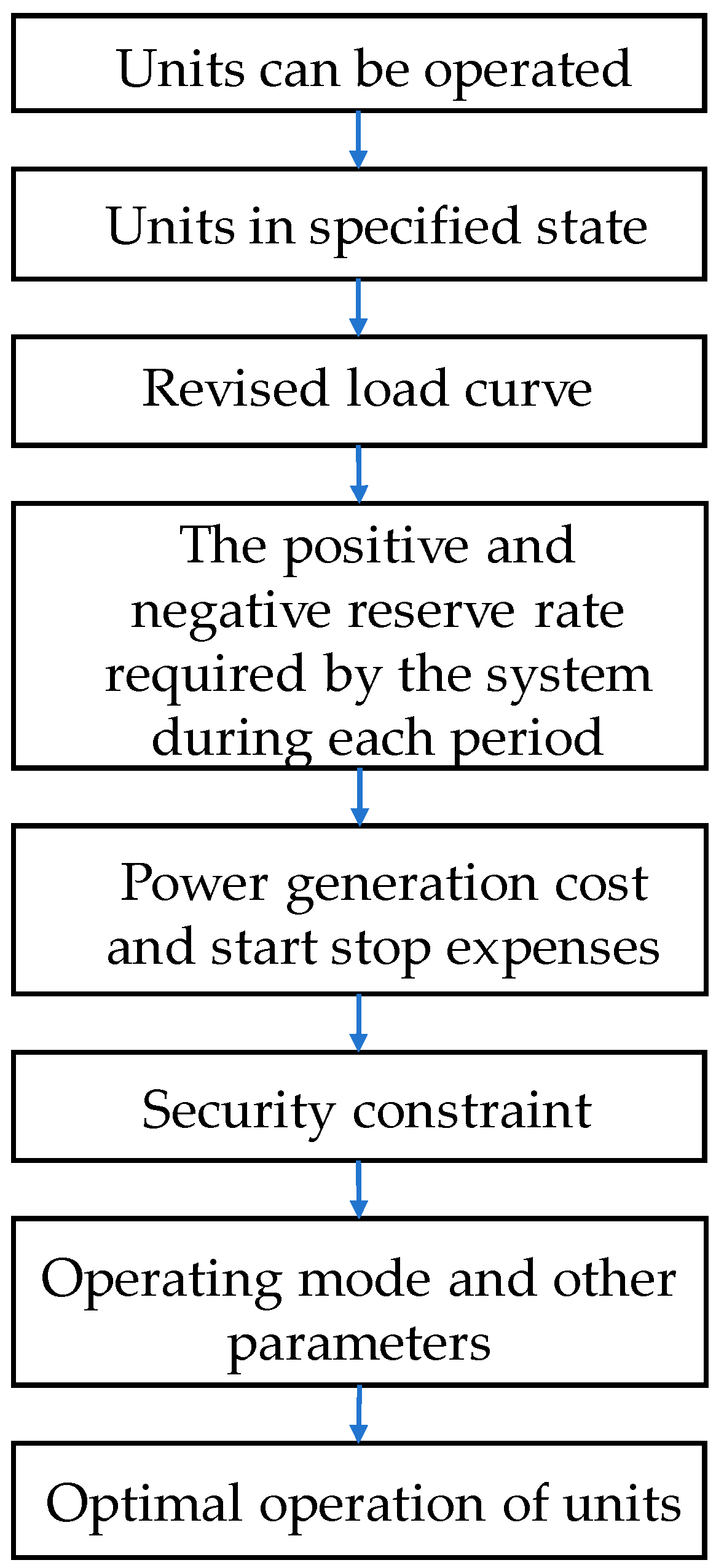
2.1. The Simulation of Power System Operation

An effective simulation of power system operation is of great significance for improving the economic benefits and power supply reliability of the power system. In addition, it also plays an important role in evaluating the development of power systems.

The simulation models for power system operation can be divided into two types: deterministic and uncertain. The deterministic model considers some constraint conditions related to time and space, such as unit start stop, peak shaving, and the constraints of the power grid. However, it only uses a limited reserve capacity of the power system to simulate unit accidents, which lack depth in the reliability analysis of the power system. The uncertain model compensates for the shortcomings of the deterministic model, but there are still some disadvantages, as follows: 1. The loss of adaptability due to excessive computational load in simulation based on the time series load curve. 2. The lack of consideration for system peak shaving in simulation based on the equivalent load duration curve.

This article adopts a deterministic model based on time series load curves, and the specific mathematical model is as seen in Figure 1.

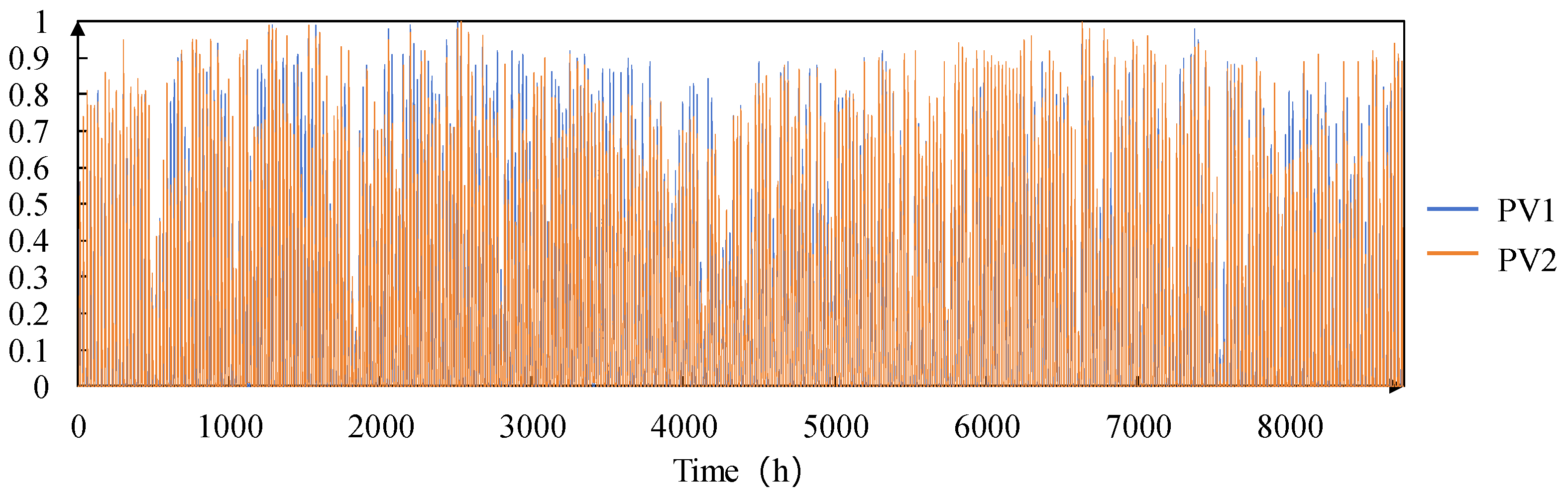
2.1.1. Output Simulation of New Energy Units

• Output simulation of wind power

$$P_{it}=n_{it}(1-{\eta }_i)C_i\left(v_{it}{k}_{ih}{k}_{im}\right)$$

(1)

In the formula, i is the order number of the wind farm, and $P_{it}$ is the simulated output of the wind farm at time t. $n_{it}$ is the number of available units. ${\eta }_i$ is the wind farm wake effect coefficient. $v_{it}$ is the wind speed sequence. $k_{ih}$ is the hourly average wind speed curve of wind farms. $k_{im}$ is the seasonal factor of wind speed in wind farms. $C_i(v)$ is the output characteristic curve of wind units, which can be obtained by Equation (2).

$$C_i(v)=\{\begin{array}{ll}0,& 0\le v<v_{in},v>v_{out}\\ \frac{v^3-v_{in}^3}{v_{out}^3-v_{in}^3}R,& v_{in}\le v\le v_{rated}\\ R,& v_{rated}\le v\le v_{out}\end{array}$$

(2)

In the formula, $v_{in}$, $v_{rated}$, and $v_{out}$ respectively represent the cut-in wind speed, rated wind speed, and cut-out wind speed of wind units. $R$ is the maximum output of wind units.

2.

Output simulation of photovoltaic panels

$$P_{jt}=P_{stc}\frac{I(R_t,k_t,I_t)}{I_{stc}}\left[1+{\alpha }_T\left(T_t-T_{stc}\right)\right]$$

(3)

In the formula, $P_t$ is the output of solar panels at time t. $P_{stc}$ is the rated output of solar panels and defined as the output of solar panels under standard conditions, in which the solar radiation intensity $I_{stc}$ = 1000 W/m² and the atmospheric temperature $T_{stc}$ = 25 °C. $R_t$ is the ratio of the solar radiation intensity on the inclined plane to the total radiation intensity on the surface plane at time t. $k_t$ is the clear sky index and defined as the ratio of solar radiation on the surface plane to the solar radiation on the outer atmosphere plane. $I_t$ is the solar radiation on the outer plane of the atmosphere without considering various random factors that weaken solar radiation. $I(R_t,k_t,I_t)$ represents the total irradiation on photovoltaic panels after considering solar radiation, clearness index, and the tilt angle of photovoltaic panels. $T_t$ is the atmospheric temperature. ${\alpha }_T$ is the power temperature coefficient of solar panels.

2.1.2. Output Simulation of New Energy Units

In order to meet the needs of different scheduling operation modes, the objective function can be selected as follows: the lowest system power generation cost, energy-saving power generation scheduling, or three public scheduling. Taking “the lowest system power generation cost” as an example, the objective function is expressed as follows:

$$\min C_{sys}={\displaystyle \sum _{t\in T}\left(\begin{array}{l}{C}_c(P_c^t)+C_f(P_f^t)+C_h(P_h^t)+C_p(P_p^t)\\ +C_w(P_w^t)+\theta C_w{P}_{wd}^t+\eta V_d{D}_d^t\end{array}\right)}+{\gamma }_f{C}_f+{\gamma }_c{C}_c$$

(4)

In the formula, T is the total number of periods during the optimization cycle. $C(P^t)$ is the operating cost of each type of unit with an output power of $P^t$ during period t, and the subscripts c, f, h, p, and w respectively represent thermal power that cannot start–stop within a day, thermal power that can start–stop within a day, hydropower, pumped storage, and new energy. $C_w$ is the cost of cutting new energy. $P_{wd}^t$ is the power of cutting new energy during period t. $D_d^t$ is the power of cutting load during period t. $V_d$ is the cutting load loss of each node. $C_f$ and $C_c$ are unit start–stop costs. θ, η, and λ are weighted coefficients.

2.1.3. Constraint Condition

• Output simulation of wind power

$${[1]}^T{P}_c^t+{[1]}^T{P}_f^t+{[1]}^T{P}_f^t+{[1]}^T{P}_w^t+{[1]}^T{D}_d^t={[1]}^T{D}^t,\forall t\in T$$

(5)

2.

Output constraints of thermal power units

The output constraints of thermal power units mainly include the upper and lower limits of the output as well as the climbing constraints of thermal power units.

$$\{\begin{array}{l}{P}_{c\min }{I}_c\le P_c^t\le P_{c\max }{I}_c\\ P_{f\min }{I}_f^t\le P_f^t\le P_{f\max }{I}_f^t\\ -\Delta P_c^{down}\le P_c^t-P_c^{t-1}\le \Delta P_c^{up}\\ -\Delta P_f^{down}\le P_f^t-P_f^{t-1}\le \Delta P_f^{up}\\ P_c^t,P_f^t,I_c,I_f^t\ge 0\\ \forall t\in T\end{array}$$

(6)

In the formula, $P_{c\min }$ and $P_{c\max }$ respectively represent the minimum and maximum output of start–stop units. $P_{f\min }$ and $P_{f\max }$ respectively represent the minimum and maximum output of no start–stop units. $I_c$ is the state variable of no start–stop units within a day. $I_f^t$ is the state variable of start–stop units within a day. $\Delta P_c^{down}$, $\Delta P_f^{down}$, $\Delta P_c^{up}$, and $\Delta P_f^{up}$ respectively represent the downhill and uphill speed of units.

3.

Output constraints of thermal power units

$$\{\begin{array}{l}\begin{array}{c}{P}_w^t+P_{wd}^t=P_{wf}^t\\ 0\le P_w^t,0\le P_{wd}^t\end{array}\\ \forall t\in T\end{array}$$

(7)

In the formula, $P_w^t$ is the output of new energy during period t. $P_{wd}^t$ is the power of cutting new energy during period t. $P_{wf}^t$ is the predicted output value of new energy during period t.

4.

Output constraints of hydropower and pumped storage units

$$\{\begin{array}{l}{P}_{h\min }\le P_h^t\le P_{h\max }\\ {\displaystyle \sum _{t=1}^T{P}_h^t}\le Q_{hydro}\\ -P_{p,pump}{I}_{p,pump}^t\le P_p^t\le I_{p,gen}^t{P}_{p,gen}\\ I_{p,pump}^t+I_{p,gen}^t=1\\ {\displaystyle \sum _{t=1}^T{I}_{p,gen}^t{P}_h^t}={\lambda }_p{\displaystyle \sum _{t=1}^T{I}_{p,pump}^t{P}_h^t}\end{array}$$

(8)

In the formula, $P_h^t$ is the output of hydropower units. $P_{h\min }$ and $P_{h\max }$ are the minimum and maximum output of hydropower units. $Q_{hydro}$ is the daily power generation of hydropower units. $P_{p,pump}$ and $P_{p,gen}$ are the maximum pumping and power generation per unit period of pumped storage units. $I_{p,pump}^t$ and $I_{p,gen}^t$ are state variables that describe the pumping or power generation of pumped storage units during period t. ${\lambda }_p$ is the efficiency of pumped storage units.

5.

Positive and negative reserve requirements of system

$${[1]}^T{D}^t+r_u^t{[1]}^T{D}^t\le {[1]}^T{P}_{c\max }^t{I}_c+{[1]}^T{P}_{f\min }^t{I}_f^t+{[1]}^T{P}_{h\min }^t+{[1]}^T{P}_{wf}^t+{[1]}^T{D}_d^t\forall t\in T$$

(9)

In the formula, $D^t$ is the load of each node during period t. $P_{c\max }^t$ is the maximum output of start–stop thermal power units during period t. $P_{f\min }^t$ is the minimum output of no start–stop thermal power units during period t. $P_{h\min }^t$ is the minimum output of hydropower units during period t. $r_u^t$ is the required positive reserve rate of the system during period t. It is worth noting that the contribution of renewable energy to the system reserve should be calculated based on its predicted output $P_{wf}^t$, and even if it is cut off, the cut off part should be included in the reserve capacity.

$${[1]}^T{P}_{c\min }^t{I}_c+{[1]}^T{P}_{f\min }^t{I}_f^t+{[1]}^T{P}_{h\min }^t+{[1]}^T{D}_d^t\le {[1]}^T{D}^t-r_d^t{[1]}^T{D}_d^t\forall t\in T$$

(10)

In the formula, $P_{c\min }^t$ is the minimum output of start–stop thermal power units during period t. $r_d^t$ is the required negative reserve rate of the system during period t. Here, the output of renewable energy is not included, which is equivalent to assuming that the minimum output of renewable energy is 0 and can be cut off at any time.

6.

Backup constraints

$$\{\begin{array}{c}{\displaystyle \sum _{c,f,h,p,w\in z}(}{P}_{c\max }{I}_c+P_{f\max }{I}_f^t+P_{h\max }+P_{p,gen}+P_{wf}^t)\\ +{\displaystyle \sum _{l\in Z^{+}}{f}_l^t-}{\displaystyle \sum _{l\in Z^{-}}{f}_l^t}+D_d^{z,t}\ge (1+r_u^{z,t})D^{z,t}\\ {\displaystyle \sum _{c,f,h,p,w\in z}(}{P}_{c\min }{I}_c+P_{f\min }{I}_f^t+P_{h\min }-P_{p,pump})\\ +{\displaystyle \sum _{l\in Z^{+}}{f}_l^t-}{\displaystyle \sum _{l\in Z^{-}}{f}_l^t}+D_d^{z,t}\le (1-r_d^{z,t})D^{z,t}\\ \forall z\in Z,\forall t\in T\end{array}$$

(11)

In the formula, Z is the total number of regions. $D^{z,t}$ is the load of region z during period t. $D_d^{z,t}$ is the cutting load of region z during period t. $r_u^{z,t}$ and $r_d^{z,t}$ respectively represent the positive and negative reserve rate of region z during period t. $Z^{+}$ and $Z^{-}$ respectively represent the collection of contact lines sent in and out of region Z. $f_l^t$ is the power flow of line l.

7.

Network constraints

$$\{\begin{array}{l}{F}_l^t=W{A}_{ngc}{P}_c^t+W{A}_{ngf}{P}_f^t+W{A}_{ngh}{P}_h^t+W{A}_{ngp}{P}_p^t\\ +W{A}_{ngw}{P}_w^t+W{D}_d^t-W{D}^t\\ -f_{l,\max }\le f_l^t\le f_{l,\max }\\ F_s^t=A_{sl}W{A}_{ngc}{P}_c^t+A_{sl}W{A}_{ngf}{P}_f^t+A_{sl}W{A}_{ngh}{P}_h^t+\\ A_{sl}W{A}_{ngp}{P}_p^t+A_{sl}W{A}_{ngw}{P}_w^t+A_{sl}W{D}_d^t-A_{sl}W{D}^t\\ -f_{s\max }\le f_s^t\le f_{s\max }\\ \forall t\in T\end{array}$$

(12)

In the formula, $W$ is the transfer distribution factor matrix of generators. $F_l^t$ and $F_s^t$ respectively represent the power flow matrices of the line and the cross-section during period t. W is the generator transfer distribution factor.$A_{ngc}$, $A_{ngf}$, $A_{ngh}$, $A_{ngp}$, and $A_{ngw}$ are node-unit correlation matrices for different types of units. $A_{sl}$ is the section-line correlation matrix.

8.

Constraints of cross-regional power transmission

$${\underset{\_}{f}}_s^t\le {\displaystyle \sum _{l\in {\Theta }_s}{f}_l^t}\le {\overline{f}}_s^t\begin{array}{cc}& \forall t\in T\end{array}$$

(13)

In the formula, ${\underset{\_}{f}}_s^t$ and ${\overline{f}}_s^t$ respectively represent the minimum and maximum power flow of the certain cross-section during period t. $\Theta s$ is the collection of lines included in section S of cross-district power transmission.

9.

Dynamic constraints

Start–stop thermal power units can only start and stop once a day, and large-capacity thermal power units are not allowed to start and stop.

2.2. Low-Carbon Demand Response

2.2.1. Low-Carbon Demand Response Mechanism

Low-carbon demand response guides electricity users to change their electricity consumption behavior by providing carbon emission information under different electricity consumption behaviors, thereby achieving a reduction in the carbon emission of the power system and promoting the integration of renewable energy.

In low-carbon demand response, the differences in carbon emission generated by different electricity consumption behaviors are mainly characterized by different carbon emission factors. The carbon emission factor used here is dynamic and must meet real-time unbiasedness.

The specific process of low-carbon demand response is as follows:

Step 1: Obtaining dynamic carbon emission factors. Based on the composition of their electricity consumption sources and the corresponding carbon emission information at different periods, the dynamic carbon emission factor of users can be calculated and displayed to users via carbon meters.

Step 2: Obtaining baseline load curve. The baseline load curve refers to the original load curve of users before applying low-carbon demand response. According to the baseline load curve and the real-time carbon emission factor, the original indirect carbon emissions of users before low-carbon demand response can be calculated.

Step 3: Optimizing users’ electricity consumption behavior. After obtaining the prediction value of carbon emission factors in the future, users can arrange their carbon reduction plans and adjust their electricity consumption behavior in the future.

Step 4: Calculating the carbon emission reduction. The actual indirect carbon emissions of users can be obtained based on the actual dynamic carbon emission factor curve and the actual power load curve. By comparing the actual indirect carbon emission with the original indirect carbon emissions, the carbon emission reduction of low-carbon demand response can be obtained.

2.2.2. Calculation Method of Regional Dynamic Average Carbon Emission Factors

The calculation method of the dynamic carbon emission factor used in this article is based on the traditional average carbon emission factor calculation method [19], but in terms of the time scale, the accounting cycle of relevant data and the calculating cycle of the indirect carbon emission factor are refined to one hour.

$$e_{i,t}=\frac{E_i+{\displaystyle \sum _{j=1}^p(e_j\times Q_j)}-{\displaystyle \sum _{k=1}^q(e_k\times Q_k)}}{Q_i+{\displaystyle \sum _{j=1}^p{Q}_j}-{\displaystyle \sum _{k=1}^q{Q}_k}}$$

(14)

In the formula, $e_{i,t}$ is the average carbon emission factor of region i during period t. $E_i$ is the total amount of direct carbon emissions generated by power generation enterprises in region i. $Q_i$ is the total electricity generated by power generation enterprises in region i. $Q_j$ and $e_j$ respectively represent the total electricity and the carbon emission factor of the j-th-type power imported from other provinces. $Q_k$ and $e_k$ respectively represent the total electricity and the carbon emission factor of the k-th-type power exported to other provinces. p is the type number of power imported from other provinces, and q is the type number of power exported to other provinces.

Based on the dynamic carbon emission factor, the carbon emission of electricity consumption by users can be calculated via the following formula:

$$E_t={\displaystyle \sum e_{i,t}\times Q_t}$$

(15)

In the formula, $E_t$ is the carbon emission of electricity consumption by the enterprise during period t. $Q_t$ is the total electricity consumption of the enterprise during period t.

2.2.3. The Benefit Evaluation Model of Low-Carbon Demand Response

The low-carbon demand response mechanism has an effect on both users and the power system. For users, they can reduce their carbon emissions by changing their electricity consumption behavior and gain tangible benefits in the carbon market. For the power system, adjusting the electricity consumption behavior of users will promote the consumption of clean energy and reduce the carbon emission of the entire power system.

This article will evaluate the carbon reduction potential of low-carbon demand response from the perspectives of both the power system and users. The specific process can be divided into four steps:

Step 1: Obtaining hourly operation data of the power system throughout the year.

Step 2: Obtaining hourly dynamic carbon emission factors of users. The specific method is as shown in Equation (14).

Step 3: Obtaining simulated results of users’ electricity consumption behavior in low-carbon demand response, assuming that the dynamic carbon emission factor prediction curve is released to users one day in advance, and users adjust their electricity consumption behavior every day. After perceiving the differences in carbon emission factors at different periods in the future, users adjust their electricity consumption behavior with the goal of maximizing their carbon emission reduction. The specific model is as follows, where Equation (16) is the objective function, and Equations (17)–(21) are the constraint conditions.

$$\Delta E_{{\mathrm{CO}}_2,d}={\displaystyle \sum _{t\in T_d}(\Delta P_{\mathrm{L},t}^{-}-\Delta P_{\mathrm{L},t}^{+})\Delta t\cdot e_{i,t}}$$

(16)

$$\{\begin{array}{l}0\le \Delta P_{\mathrm{L},t}^{+}\le u_{\mathrm{L},t}^{+}\cdot \Delta {\overline{P}}_{\mathrm{L},t}\\ 0\le \Delta P_{\mathrm{L},t}^{-}\le u_{\mathrm{L},t}^{-}\cdot \Delta {\overline{P}}_{\mathrm{L},t}\end{array}$$

(17)

$$u_{\mathrm{L},t}^{+}+u_{\mathrm{L},t}^{-}\le 1$$

(18)

$$P_{\mathrm{L},t}+\Delta P_{\mathrm{L},t}^{+}\le {\overline{P}}_{L,t}$$

(19)

$$\Delta P_{\mathrm{L},t}^{-}\le P_{\mathrm{L},t}$$

(20)

$$\left|{\displaystyle \sum _{t\in T_d}(\Delta P_{\mathrm{L},t}^{+}-\Delta P_{\mathrm{L},t}^{-})}\right|\le \Delta {\overline{P}}_{\mathrm{L}}$$

(21)

In these formulas, $\Delta E_{{\mathrm{CO}}_2,d}$ is the daily carbon reduction of electricity users. $T_d$ is the total number of hours during the accounting day. $\Delta P_{\mathrm{L},t}^{+}$ and $\Delta P_{\mathrm{L},t}^{-}$ respectively represent the increase and decrease in the load of electricity users during period t after low-carbon demand response. $\Delta {\overline{P}}_{\mathrm{L},t}$ is the upper limit of load that electricity users can adjust during period t. $u_{\mathrm{L},t}^{+}$ and $u_{\mathrm{L},t}^{-}$ are 0 or 1 variables that indicate whether the user is in an increased load state or a decreased load state. $P_{\mathrm{L},t}$ and ${\overline{P}}_{L,t}$ respectively represent the baseline load and the maximum load of users during period t. $\Delta {\overline{P}}_{\mathrm{L}}$ is the maximum value of daily load variation for electricity users.

Step 4: Calculating the benefits of carbon reduction. Based on the changes in the electricity consumption of users, the carbon reduction of users after low-carbon demand response and the benefits of it in the carbon market can be calculated by equations as follows:

$$\Delta E_{\mathrm{C}{\mathrm{O}}_2,T}={\displaystyle \sum _{t\in T_T}(\Delta P_{\mathrm{L},t}^{-}-\Delta P_{\mathrm{L},t}^{+})\Delta t\cdot e_{i,t}}$$

(22)

$$R_{\mathrm{C}{\mathrm{O}}_2,T}=\Delta E_{\mathrm{C}{\mathrm{O}}_2,T}\cdot p_{{\mathrm{CO}}_2}$$

(23)

In these formulas, $\Delta E_{\mathrm{C}{\mathrm{O}}_2,T}$ is the carbon reduction of users during the accounting cycle T. $T_T$ is the total number of hours during accounting cycle T. $R_{\mathrm{C}{\mathrm{O}}_2,T}$ is the benefits of carbon reduction during accounting cycle T. $p_{{\mathrm{CO}}_2}$ is the price of CO₂.

3. Results and Discussion

3.1. Empirical Analysis of North China Power Grid

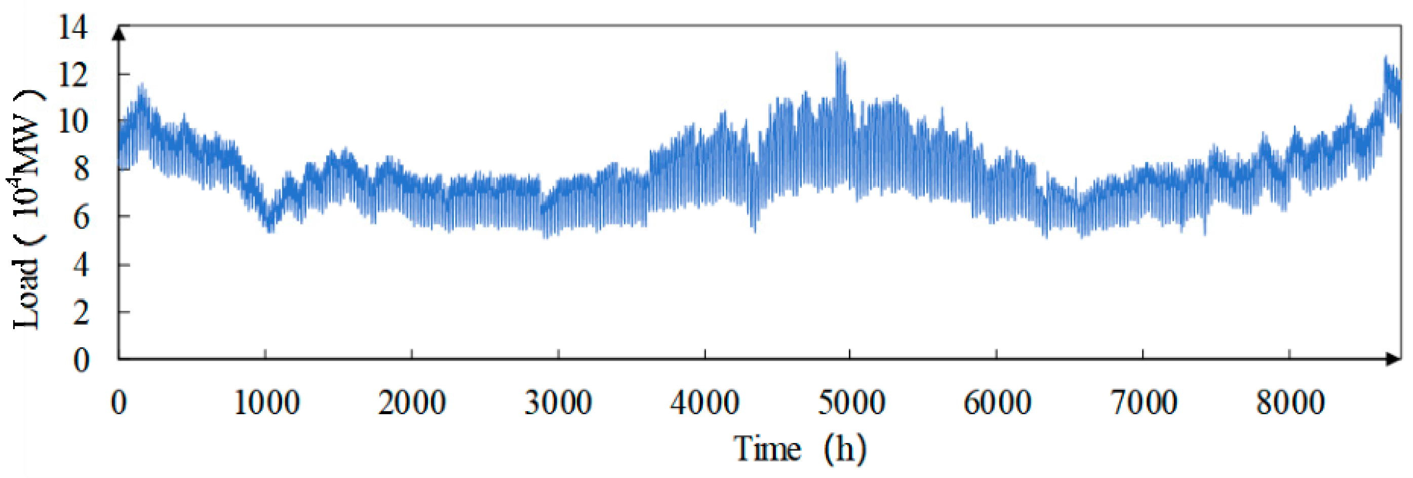
3.1.1. Introduction to the Example System

This article carries out an empirical analysis of low-carbon optimization and low-carbon demand response for the 2040 system planning scheme of the North China Power Grid. The power installed capacity and load parameters of the North China Power Grid in 2040 are obtained by combining the simulation model of power system operation in Section 2 with the carbon peak and carbon neutrality goals of the North China Power Grid. The power unit consists of thermal power, heating gas turbines, pumped storage, and photovoltaic and wind power. The situation of power installed capacity in the example is shown in

Table 1. Overall installed capacity of North China Power Grid in 2040.

Unit Type	Installed Capacity (MW)
Thermal power	129,912
Heating gas turbines	39,178
Wind power	68,300
Photovoltaic	129,000
Pumped storage	90,470
Other energy storage	20,600

,

Table 2. Wind power installed capacity.

Wind Region	Wind Power Installed Capacity (MW)
Wind region 1	17,758
Wind region 2	50,542

and

Table 3. Photovoltaic installed capacity.

Photovoltaic Region	Photovoltaic Installed Capacity (MW)
Photovoltaic region 1	24,588
Photovoltaic region 2	77,862

.

The output of wind power and photovoltaic power is obtained by simulation based on the characteristics of wind and photovoltaic resources as well as the characteristics of wind and photovoltaic units in North China. The output curves of wind power and photovoltaic power are shown in Figure 2 and Figure 3. The system load is obtained by simulation based on the historical load parameters and expected load growth of the North China Power Grid. The load curve is shown in Figure 4.

Figure 2 and Figure 3 respectively show the per unit value curves of wind power and photovoltaic power in the entire region of the North China Power Grid in 2040.

Wind power generation has strong intermittency and volatility and presents significant uncertainty, and its output varies greatly. Photovoltaic power generation has strong periodicity due to the strong influence of sunlight intensity, and its output mainly concentrates from 8:00 to 17:00 per day.

Figure 4 shows the overall regional load curve of the North China Power Grid in 2040. The detailed data corresponding to the load curve were calculated through the Grid Optimization Planning Tools (GOPT) developed by Tsinghua University. It can be seen that the peak load of electricity consumption is mainly concentrated in summer and winter when cooling and heating supply are required.

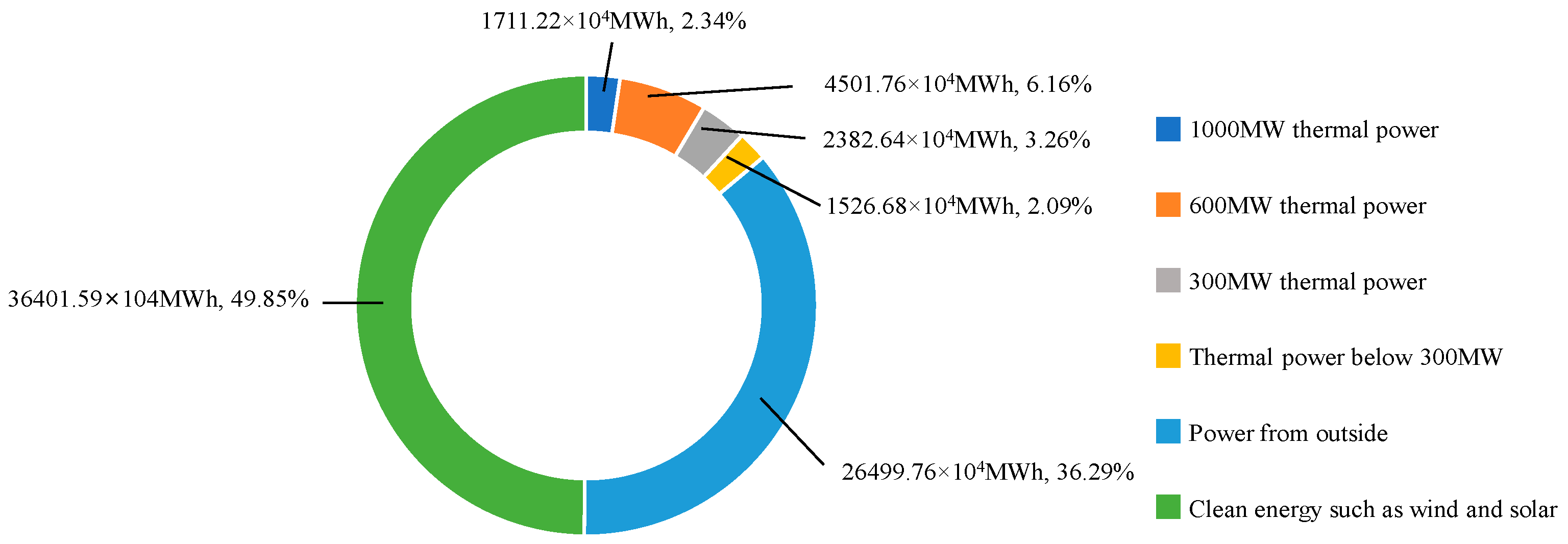
3.1.2. Analysis of Low-Carbon Optimization Results for North China Power Grid in 2040

Based on the simulation model of power system operation and the planning scheme of the North China Power Grid in 2040, the results and analysis of low-carbon optimization for the North China Power Grid in 2040 are as follows.

Figure 5 shows the proportion of various types of power generation for the North China Power Grid in 2040. With the rapid development of new energy generation and the demand for carbon emission reduction, by 2040, clean energy power such as wind and solar as well as power from outside respectively account for 49.85% and 36.29% of the annual electricity consumption for the North China Power Grid. And the proportion of thermal power is only 13.86%.

Table 4. Annual renewable energy consumption of North China Power Grid in 2040.

	Wind Power	Photovoltaic	Total
Annual total power generation/104 MWh	18,970.24	21,297.66	40,267.90
Annual total power abandonment/104 MWh	3033.18	833.13	3866.31
Annual consumption rate%	84.01	96.09	90.40

shows the annual renewable energy consumption of the North China Power Grid in 2040. The annual consumption rate of wind power and PV power is 84.01% and 96.09%, respectively. And the annual renewable energy consumption of the power grid is 90.40%, which indicates that the North China Power Grid can realize the efficient consumption of renewable energy in 2040 scenarios. Figure 6 shows the variation curve of the annual abandonment rate of wind and solar power for the North China Power Grid in 2040. The system has less power abandonment in winter and summer because of the higher load. And the pressure of consumption increases in spring and fall due to the lower load.

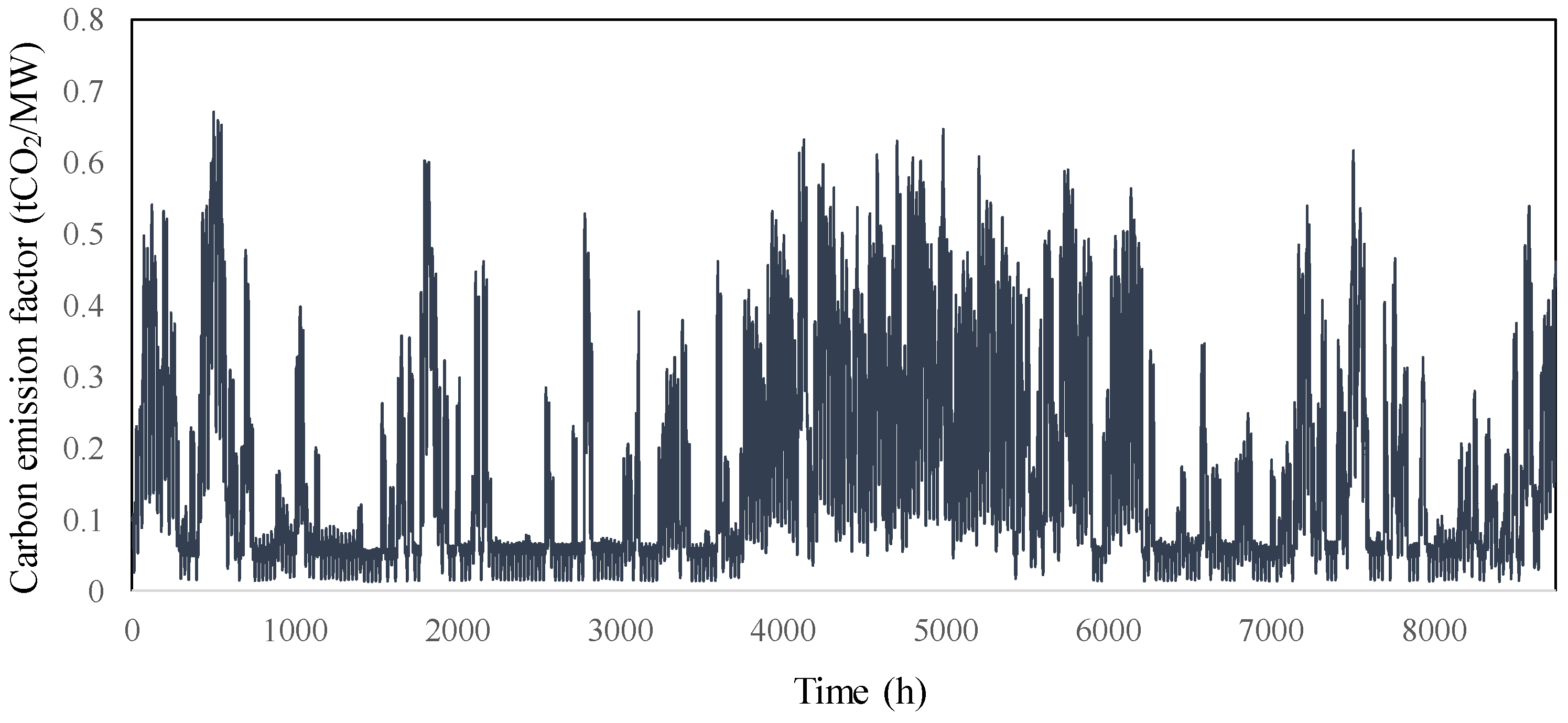
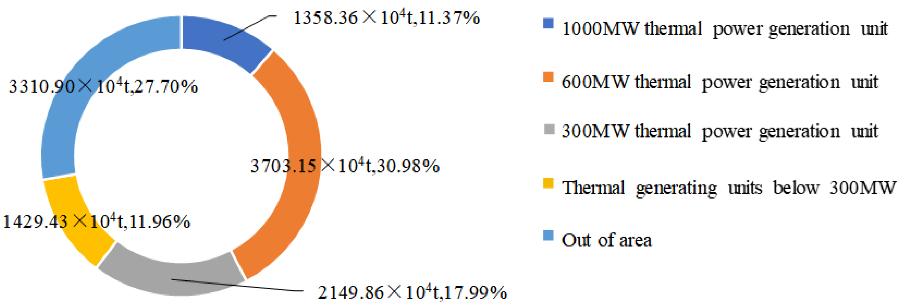
3.1.3. Carbon Emission Characteristics Analysis of Low-Carbon Optimization for North China Power Grid in 2040

Inputting parameters such as the types and carbon emission factors of units participating in the power generation plan, the output of units and the amount of power from outside in each period, and the load of the system in each period, the carbon emission parameters of the system for the North China Power Grid such as the dynamic carbon emission factor of electricity consumption, the carbon emissions and their proportions of various types of power sources, and the carbon emission proportions of each type of unit can be obtained by solving. This article carries out system operation simulation based on the power grid planning scenario of the North China Power Grid in 2040 and solves the system carbon emissions under the planning scenario as follows.

Figure 7 shows the dynamic carbon emission factor curve for the entire year 8760 h of the North China Power Grid in 2040. And Figure 8 shows the curve of annual carbon emission from power generation and power from outside of the North China Power Grid in 2040. In spring and autumn, despite that the abandonment rate of wind power and PV power is higher, the output of thermal power units is lower due to the reduced load, which results in a lower level of the carbon emission factor and carbon emissions for the North China Power Grid. On the contrary, in winter and summer, despite that the efficient consumption of new energy power in the system has been achieved, the output of thermal power increases significantly due to the increased load, which results in the North China Power Grid still exhibiting a higher level of carbon emission characteristics.

Figure 9 shows the carbon emissions from power generation and power from outside of the North China Power Grid for the whole year of 2040. The carbon emission factor of power from outside is at a low level, and the carbon emissions of the North China Power Grid are mainly generated by thermal power units. In the context of a high proportion of new energy power being integrated into the power system in the future, retaining some thermal power units is of great significance for supporting the safe and stable operation of the North China Power Grid. Therefore, promoting the transformation of thermal power units and deepening the application of carbon capture technology will become an important method to promote the low-carbon transformation of the North China Power Grid.

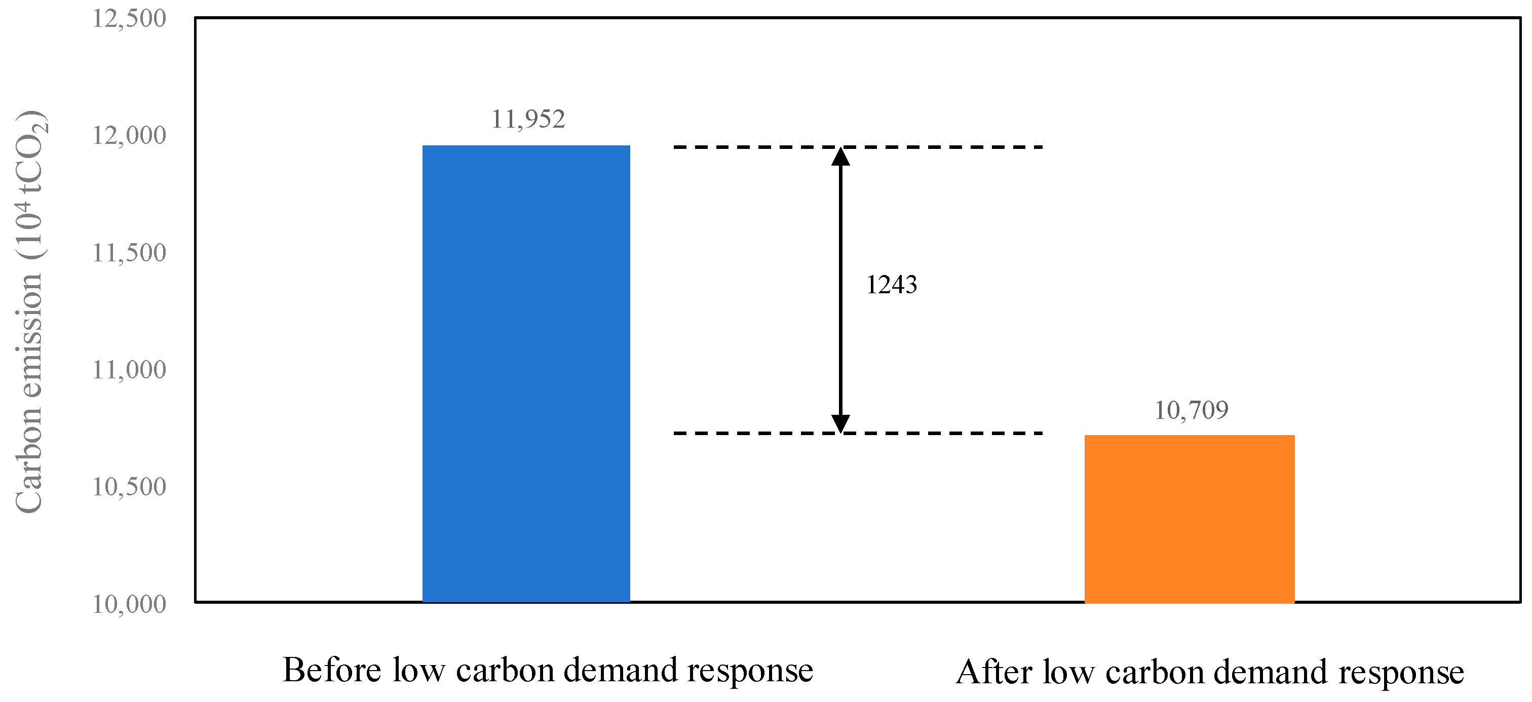
3.1.4. Benefit Analysis of Low-Carbon Demand Response of North China Power Grid in 2040

Based on the dynamic carbon emission factor data throughout the entire year 8760 h of the North China Power Grid in 2040 shown above, the carbon reduction benefits of the North China Power Grid in 2040 can be obtained via the benefit evaluation model mentioned in Section 3. Assuming that 5% of loads in the North China Power Grid participate in low-carbon demand response, the carbon reduction benefits of the North China Power Grid in 2040 after low-carbon demand response would reach 1243 × 10⁴ tCO₂.

Figure 10 shows the carbon reduction benefits of the North China Power Grid in 2040 under the mechanism of low-carbon demand response. It can be seen that after carrying out low-carbon demand response, the annual carbon reduction in the North China Power Grid reached 12.43 million tons CO₂, which will bring huge environmental and economic benefits to the North China region.

Figure 11 shows the carbon reduction in each province in the North China Power Grid after low-carbon demand response by 2040. Among the five provinces of North China, Shandong has the greatest potential of carbon reduction, which accounts for 57.36% of the total carbon reduction in the North China Power Grid. And Hebe also has a significant potential of carbon reduction, which accounts for 21.64% of the total carbon reduction in the North China Power Grid.

4. Conclusions

This article first delved into a simulation model of power system operation: a deterministic simulation model of power system operation based on time series load curves. And then, it proposed a carbon reduction mechanism of the power system which can guide system users to respond actively and reduce the carbon emission of the system, named the mechanism of low-carbon demand response.

Finally, based on the planning scheme and carbon peak and carbon neutrality goals of the North China Power Grid, this article calculated the simulation scenario of system operation for the North China Power Grid in 2040 via the deterministic simulation model of power system operation based on time series load curves. Furthermore, based on this simulation scenario, a carbon reduction benefit analysis of low-carbon demand response for the North China Power Grid in 2040 was carried out.

The results of operation simulation and carbon reduction benefits analysis indicate the following:

• Under the context of low-carbon development, the North China Power Grid will own a high proportion of clean energy electricity such as wind and solar power by 2040.
• Despite owning a relatively high proportion of new energy electricity in 2040, the North China Power Grid still exhibits high carbon emission characteristics in winter and summer. Therefore, it is necessary to continue developing new energy electricity and deepening the application of carbon capture technology to further optimize the energy structure.
• The low-carbon demand response can bring huge carbon reduction benefits to the system of the North China Power Grid.
• Regions with a greater potential of load regulation and a larger peak valley difference in the carbon emission factor have better carbon reduction benefits brought by low-carbon demand response: the carbon reduction benefit of Shandong in 2040 is better than that of other provinces in North China under the mechanism of carbon demand response.

References

1. Gan, T.; Zhou, Z.; Li, S.; Tu, Z. Carbon emission trading, technological progress, synergetic control of environmental pollution and carbon emissions in China. J. Clean. Prod. 2024, 442, 141059. [Google Scholar] [CrossRef]
2. Shu, Y.; Zhao, Y.; Zhao, L.; Qiu, B.; Liu, M.; Yang, Y. Study on low carbon energy transition path toward carbon peak and carbon neutrality. Proc. CSEE 2023, 43, 1663–1672. [Google Scholar]
3. Li, Z.; Zhang, D.; Pan, L.; Li, T.; Gao, J. Low-Carbon Transition of China’s Energy Sector and Suggestions with the Carbon-Peak and Carbon-Neutrality Target. J. Chin. Soc. Power Eng. 2021, 41, 905–909. [Google Scholar]
4. Li, Z.; Chen, S.; Dong, W.; Liu, P.; Du, E.; Ma, L.; He, J. Low carbon transition pathway of power sector under carbon emission constraints. Proc. CSEE 2021, 41, 3987–4001. [Google Scholar]
5. Hou, J.; Sun, W.; Xiao, J.; Jin, C.; Du, E.; Huang, J. Collaborative optimization of key technology progress and low-carbon transition of power systems. Autom. Electr. Power Syst. 2022, 46, 1–9. [Google Scholar]
6. Liu, Z.; Li, M.; Virguez, E.; Xie, X. Low-carbon transition pathways of power systems for Guangdong–Hongkong–Macau region in China. Energy Environ. Sci. 2024, 17, 307–322. [Google Scholar] [CrossRef]
7. Yuan, G.; Liu, H.; Yu, J.; Liu, X.; Fang, F. Combined heat and power optimal dispatching in virtual power plant with carbon capture cogeneration unit. Proc. CSEE 2022, 42, 4440–4449. [Google Scholar]
8. Cui, Y.; Deng, G.; Wang, Z.; Wang, M.; Zhao, Y. Low-carbon economic scheduling strategy for power system with concentrated solar power plant and wind power considering carbon trading. Electr. Power Autom. Equip. 2021, 41, 232–239. [Google Scholar]
9. Chen, Z.; Lu, Y.; Xing, Q.; Chen, X.; Leng, Z. Dispatch analysis of power system considering carbon quota for electric vehicle. Autom. Electr. Power Syst. 2019, 43, 44–51. (In Chinese) [Google Scholar]
10. Luo, Z.; Qin, J.; Liang, J.; Shen, F.; Liu, H.; Zhao, M.; Wang, J. Day-ahead optimal scheduling of integrated energy system with carbon-green certificate coordinated trading mechanism. Electr. Power Autom. Equip. 2021, 41, 248–255. [Google Scholar]
11. Che, Q.; Wu, Y.; Zhu, Z.; Lou, S. Carbon trading based optimal scheduling of hybrid energy storage system in power systems with large-scale photovoltaic power generation. Autom. Electr. Power Syst. 2019, 43, 76–83. [Google Scholar]
12. Olsen, D.; Kirschen, D. Profitable emissions-reducing energy storage. IEEE Trans. Power Syst. 2019, 35, 1509–1519. [Google Scholar] [CrossRef]
13. Hou, Q.; Du, E.; Zhang, N.; Kang, C. Impact of high renewable penetration on the power system operation mode: A data-driven approach. IEEE Trans. Power Syst. 2019, 35, 731–741. [Google Scholar] [CrossRef]
14. Wu, H.; Du, E.; Men, K.; Yang, L.; Su, L.; Lu, S.; Luo, O. A low-carbon oriented energy-saving and economic operation evaluation system. Power Syst. Technol. 2015, 5, 1179–1185. [Google Scholar]
15. Qiang, S.; Wang, G.; Min, Y.; Su, P. Joint low-carbon economic dispatch of power system considering reward-penalty ladder carbon trading and demand response. In Proceedings of the 2023 7th International Conference on Smart Grid and Smart Cities (ICSGSC), Lanzhou, China, 22–24 September 2023; IEEE: Piscataway, NJ, USA, 2023; pp. 561–566. [Google Scholar]
16. Sun, Z.; Sun, Y.; Liu, M.; Song, Y. Low-carbon operation strategy of power system considering carbon flow demand response. Electr. Power 2023, 56, 95–103. [Google Scholar]
17. Chen, Y.; Zhang, N.; Kang, C.; Meng, J.; Yan, H. Low Carbon Transmission Expansion Planning Considering Demand Side Management. Autom. Electr. Power Syst. 2016, 40, 61–69. [Google Scholar]
18. Yang, Y.; Liu, J.; Xu, X.; Xie, K. Two-Stage Low-Carbon Optimal Scheduling of Power System Based on Carbon Flow Theory and Demand Response. In Proceedings of the 2023 Panda Forum on Power and Energy (PandaFPE), Chengdu, China, 27–30 April 2023; IEEE: Piscataway, NJ, USA, 2023; pp. 1030–1034. [Google Scholar]
19. Tian, Z.; Yang, Z.; Cai, R. Analysis of Guangdong carbon emissions from energy consumption and the driving factors of its intensity change. China Environ. Sci. 2015, 35, 1885–1891. [Google Scholar]
Figure 1. Simulation flow of power system operation.
Processes 12 01324 g001
Figure 2. Per unit curve of wind power generation for North China Power Grid in 2040.
Processes 12 01324 g002
Figure 3. Per unit curve of PV power generation for North China Power Grid in 2040.
Processes 12 01324 g003
Figure 4. Regional load curve of North China Power Grid in 2040.
Processes 12 01324 g004
Figure 5. The proportion of various types of power generation for the North China Power Grid in 2040.
Processes 12 01324 g005
Figure 6. Variation curve of annual wind and photovoltaic abandonment of North China Power Grid in 2040.
Processes 12 01324 g006
Figure 7. The dynamic carbon emission factor curve of the North China Power Grid in 2040.
Processes 12 01324 g007
Figure 8. The annual carbon emission curve of power generation and power from outside for the North China Power Grid in 2040.
Processes 12 01324 g008
Figure 9. The proportions of annual carbon emission from power generation and power from outside for the North China Power Grid in 2040.
Processes 12 01324 g009
Figure 10. The carbon reduction benefits of the North China Power Grid in 2040 under the mechanism of low-carbon demand response.
Processes 12 01324 g010
Figure 11. The carbon reduction of each province in the North China Power Grid after low-carbon demand response by 2040.
Processes 12 01324 g011