Investigating Magnetohydrodynamic Motions of Oldroyd-B Fluids through a Circular Cylinder Filled with Porous Medium

Abstract

We analytically investigated the magnetohydrodynamic motions of electrically conductive, incompressible Oldroyd-B fluids through an infinite circular cylinder filled with a porous medium. A general expression was established for the dimensionless velocity of fluid as a cylinder moves along its symmetry axis with an arbitrary velocity; the expression can generate exact solutions for any motion of this fluid type, solving the discussed problem. Special cases were considered and validated through graphical investigation to illustrate important characteristics of fluid behavior. In application, this is the first presentation of an exact general expression for non-trivial shear stress related to the magnetohydrodynamic motions of Oldroyd-B fluids when a longitudinal time-dependent shear stress is applied to the fluid by a cylinder. Solutions for the motions of rate-type fluids are lacking. The graphical representations show that in the presence of a magnetic field or porous medium, fluids flow more slowly and the steady state is reached earlier.

1. Introduction

The constitutive equations of incompressible Oldroyd-B fluids (IOBFs), as introduced by Oldroyd [1], are given by the following relations:

$$\mathit{T}=-p\mathit{I}+\mathit{S}, \left(1+\lambda \frac{D}{Dt}\right)\mathit{S}=2\mu \left(1+{\lambda }_r\frac{D}{Dt}\right)\mathit{D},$$

(1)

in which T is the Cauchy stress tensor, S is the extra-stress tensor, $\mathit{D}$ is the rate of deformation tensor, I is the identity tensor, p is the hydrostatic pressure, $\mu$ is the dynamic viscosity, $\lambda$ and ${\lambda }_r$ are relaxation and retardation times, respectively, and $D/Dt$ denotes the time upper-convected derivative [2]. If the constant ${\lambda }_r=0$ or ${\lambda }_r=\lambda =0$, the governing Equation (1) defines incompressible Maxwell or Newtonian fluids, respectively.

Oldroyd-B fluids store energy like a linear elastic solid but their dissipation corresponds to a mixture of two viscoelastic fluids. They can describe stress relaxation and the normal stress differences in simple shear flows but cannot describe shear thinning or shear thickening in the responses of some polymeric fluids. However, the Oldroyd-B model is amenable to analysis and can describe the behavior of many polymeric liquids. The first exact solutions for unsteady motions of these fluids in cylindrical domains seem to be those of Waters and King [3]. Interesting results regarding unsteady motions of incompressible Oldroyd-B fluids in such a domain have been obtained by Rajagopal and Bhatnagar [4], Wood [5], Fetecau [6], Fetecau et al. [7], McGinty et al. [8], Khan et al. [9], Imran et al. [10] and Ullah et al. [11].

The motions of fluids in the presence of a magnetic field have many engineering applications like MHD generators, polymer manufacturing, biological fluids, plasma studies, hydrology, etc. The interplay between a magnetic field and a moving electrically conductive fluid impacts chemistry and physics applications. The influence of a magnetic field on the Couette flow of a viscous fluid was previously investigated by Tao [12] and Katagiri [13]. Exact solutions for MHD motions of electrical conductive incompressible Oldroyd_B fluids (ECIOBs) in rectangular domains have been obtained, for instance, by Zahid et al. [14] and Ghosh et al. [15]. On the other hand, the dynamics of a fluids’ motion through a porous medium has multiple applications in geophysics, astrophysics, the petroleum industry, oil reservoir technology, composite manufacturing processes, and agricultural engineering. Exact solutions for magnetohydrodynamic (MHD) motions of electrical conduction incompressible Oldroyd-B fluids (ECIOBFs) through porous media in cylindrical domains have been derived by Hayat et al. [16,17] and Hamza [18]. Recently, some of these results were extended to fractional Oldroyd-B fluids by Mohammed and Salih [19], but their results are incorrect in relation to (2) and (3). Interesting applications of the non-Newtonian motions can be found in the recent work of Ahadi et al. [20].

The main purpose of this work is to completely express ECIOBF motion through an infinite circular cylinder that moves along its axis with an arbitrary velocity when magnetic and porous effects are taken into consideration. A general expression of the dimensionless velocity field is determined by means of the Laplace and finite Hankel transforms, generating exact solutions for any motion of this fluid type. For illustration, particular cases are considered, and the results are graphically proved. A governing equation for the non-trivial shear stress of MHD unsteady ECIOBF motions is obtained for the first time, and the general expression considers shear stress prescribed on the boundary. Finally, the influence of magnetic field and the porous medium on the fluid behavior is graphically depicted and discussed.

2. Basic Equations

The balance of linear momentum for isothermal unsteady MHD motions of incompressible fluids through a porous medium is characterized by the equation [16,21]

$$\rho \frac{d\mathit{w}}{dt}=-\nabla p+div\mathit{S}+\mathit{R}+{\mathit{F}}_e,$$

(2)

where $\rho , \mathit{w}, \mathit{R}$, and ${\mathit{F}}_e={\rho }_e\mathit{E}+\mathit{j}\times \mathit{B}$ are the fluid density, the velocity vector, Darcy’s resistance, and the force arising from the excess charge density ${\rho }_e$ and the induced magnetic effect due to the motion of the conducting fluid through a magnetic field. The two terms of the force ${\mathit{F}}_e$ are the electrostatic force on the excess charges due to the presence of an imposed electric field $\mathit{E}$, respectively, and the force due to the interaction of the electric current $\mathit{j}$ in the fluid and the magnetic induction $\mathit{B}$.

Along with Equation (2), the following version of Maxwell’s equations is considered:

$$\mathit{B}=\tilde{\mu }\mathit{H}, \nabla \cdot \mathit{H}=0, \mathrm{curl}\mathit{H}=4\pi \mathit{J}, \nabla \cdot \mathit{J}=0,$$

(3)

where $\tilde{\mu }$ is the magnetic permeability, $\mathit{H}$ is magnetic intensity, and $\mathit{J}$ is total electric current density. The electric current densities $\mathit{j}$ and $\mathit{J}$ have distinct locations and actions. The electric current density $\mathit{j}$ is given by the generalized Ohm’s law [21]

$$\mathit{j}=\sigma (\mathit{E}+\tilde{\mu }\mathit{w}\times \mathit{H})=\sigma (\mathit{E}+\mathit{w}\times \mathit{B}),$$

(4)

where $\sigma$ is the electrical conductivity and is considered to be constant in the present paper.

When an electrically conducting fluid moves through the magnetic lines of force generated by a magnetic field ${\mathit{B}}_0$, the electrical charges are accelerated and their motion gives rise to the electric current $\mathit{j}$ in the fluid. The magnetic induction ${\mathit{B}}_0$ is perturbed to the value $\mathit{B}={\mathit{B}}_0+\mathit{b}$. The vector field $\mathit{b}$ is the induced magnetic field resulting from the electric current in the fluid.

In the present analysis, the following are assumed [21]:

-

The applied magnetic field ${\mathit{B}}_0$ is perpendicular to the velocity field;

-

Permeability $\tilde{\mu }$ is constant throughout the fluid;

-

The excess charge density ${\rho }_e$ and imposed electric field $\mathit{E}$ are equal to zero;

-

The induced magnetic field $\mathit{b}$ is negligible in comparison with the applied magnetic field ${\mathit{B}}_0$.

In the above hypotheses, the magnetic force can be linearized, and it has the following expression:

$${\mathit{F}}_e=\mathit{J}\times \mathit{B}=-\sigma B_0^2\mathit{w},$$

(5)

Darcy’s resistance for motions of ECIOBFs has to satisfy the relation [16]

$$\left(1+\lambda \frac{\partial }{\partial t}\right)\mathit{R}=-\mu \frac{\varphi }{k}\left(1+{\lambda }_r\frac{\partial }{\partial t}\right)\mathit{w},$$

(6)

where $\varphi$ ($0<\varphi <1$) and k ($>0$) are the porosity and the permeability of porous medium.

In the following, we shall consider isothermal MHD motions of ECIOBFs through a porous medium in an infinite, horizontal, circular cylinder, where fluid velocity vector w, in a convenient cylindrical coordinate system r, $\theta$, and z, has the form

$$\mathit{w}=\mathit{w}(r,t)=w(r,t){\mathit{e}}_z,$$

(7)

where ${\mathit{e}}_z$ is the unit vector along the z-direction. Assuming that the extra-stress tensor S as well as the velocity vector w are functions of r and t only, and that the fluid was at rest up to the initial moment $t=0$, it is not difficult to show that the components $S_{r\theta }, S_{\theta \theta }, S_{\theta z}$ and $S_{zz}$ of the extra-stress tensor S are zero [16]. Moreover, the non-trivial shear stress $\eta (r,t)=S_{rz}(r,t)$ has to satisfy the following partial differential equation:

$$\left(1+\lambda \frac{\partial }{\partial t}\right)\eta (r,t)=\mu \left(1+{\lambda }_r\frac{\partial }{\partial t}\right)\frac{\partial w(r,t)}{\partial r}.$$

(8)

The continuity equation is identically satisfied while, in the absence of a pressure gradient in the z-direction, the governing Equations (2) and (6) take the following reduced forms [16]:

$$\rho \frac{\partial w(r,t)}{\partial t}=\frac{\partial \eta (r,t)}{\partial r}+\frac{1}{r}\eta (r,t)-\sigma B^{2}w(r,t)+\Re (r,t),$$

(9)

$$\left(1+\lambda \frac{\partial }{\partial t}\right)\Re (r,t)=-\mu \frac{\varphi }{k}\left(1+{\lambda }_r\frac{\partial }{\partial t}\right)w(r,t),$$

(10)

where $\Re$ is the non-trivial component of R.

3. Problem Presentation

Let us assume that an ECIOBF is at rest in a porous medium in an infinite horizontal circular cylinder of radius $R_0$. At the moment $t=0^{+}$, the cylinder begins to slide along its axis with the time-dependent velocity $Vh(t)$. The function $h(\cdot )$ is piecewise continuous, and $h(0)=0$ while V is a constant velocity. Owing to the shear, the fluid begins to move and its velocity vector w is characterized by Equation (7). The governing equations corresponding to this motion are given by Relations (8)–(10), while the initial and boundary conditions are

$$w(r,0)=0, \eta (r,0)=0, R(r,0)=0; 0<r<R_0,$$

(11)

$$w(R_0,t)=Vh(t); t\ge 0.$$

(12)

Introducing the next non-dimensional functions, variables, and parameters

$$w^{\ast }=\frac{1}{V}w, {\eta }^{\ast }=\frac{R_0}{\mu V}\eta , R^{\ast }=\frac{R_0^2}{\mu V}R, r^{\ast }=\frac{1}{R_0}r, t^{\ast }=\frac{\nu }{R_0^2}t, h^{\ast }(t^{\ast })=h\left(\frac{R_0^2}{\nu }{t}^{\ast }\right), \alpha =\frac{\nu }{R_0^2}\lambda , \beta =\frac{\nu }{R_0^2}{\lambda }_r,$$

(13)

and neglecting the star notation, one obtains the dimensionless forms

$$\left(1+\alpha \frac{\partial }{\partial t}\right)\eta (r,t)=\left(1+\beta \frac{\partial }{\partial t}\right)\frac{\partial w(r,t)}{\partial r}; 0<r<1, t>0,$$

(14)

$$\frac{\partial w(r,t)}{\partial t}=\frac{\partial \eta (r,t)}{\partial r}+\frac{1}{r}\eta (r,t)-Mw(r,t)+R(r,t)=0; 0<r<1, t>0,$$

(15)

$$\left(1+\alpha \frac{\partial }{\partial t}\right)R(r,t)=-K\left(1+\beta \frac{\partial }{\partial t}\right)w(r,t); 0<r<1, t>0,$$

(16)

of the governing equations. In the above relations, $\nu =\mu /\rho$ is the cinematic viscosity of the fluid, and the magnetic and porous parameters M and K are defined by the relations

$$M=\frac{\sigma B^2}{\rho }\frac{R_0^2}{\nu }=\frac{R_0^2}{\mu }\sigma B^2, K=\frac{\varphi }{k}{R}_0^2.$$

(17)

The corresponding initial conditions have the same forms as in Equation (11), while the non-dimensional boundary condition is

$$w(1,t)=h(t); t\ge 0.$$

(18)

To find analytic solutions for the motion discussed problem, we have to solve the system of partial differential Equations (14)–(16) with the initial and boundary conditions (11) and (18), respectively. The obtained results can be used to provide exact solutions for any motion of this type. Consequently, the considered motion is completely solved. To illustrate the influences of magnetic field and porous medium on the fluid motion, particular cases are considered. As the motions become steady in time, their starting velocities are presented as a sum of their steady-state and transient components. Finally, based on an important remark regarding the non-trivial shear stress for MHD unsteady motions of ECIOBFs, exact solutions that apply to the shear stress of fluids are provided for motions induced by a cylinder.

4. Analytic Solutions

In order to determine the exact analytic solutions, the Laplace and finite Hankel transforms are used. Applying the Laplace transform to Equations (14)–(16) and considering the initial Conditions (11), one finds the transform equations

$$(\alpha s+1)\tilde{\eta }(r,s)=(\beta s+1)\frac{\partial \tilde{w}(r,s)}{\partial r}; 0<r<1,$$

(19)

$$s\tilde{w}(r,s)=\frac{\partial \tilde{\eta }(r,s)}{\partial r}+\frac{1}{r}\tilde{\eta }(r,s)-M\tilde{w}(r,s)+\tilde{R}(r,s); 0<r<1,$$

(20)

$$(\alpha s+1)\tilde{R}(r,s)=-K(\beta s+1)\tilde{w}(r,s); 0<r<1,$$

(21)

in which $\tilde{w}(r,s)$, $\tilde{\eta }(r,s)$, and $\tilde{R}(r,s)$ are the Laplace transforms of $w(r,t)$, $\eta (r,t)$, and $R(r,t)$ and s is the transform parameter. The function $\tilde{w}(r,s)$ has to satisfy the condition

$$\tilde{w}(1,s)=\tilde{h}(s),$$

(22)

where $\tilde{h}(s)$ is the Laplace transform of $h(t)$.

Eliminating $\tilde{\eta }(r,s)$ and $\tilde{R}(r,s)$ between Equations (19)–(21), one obtains the next ordinary differential equation:

$$\frac{{\partial }^2\tilde{w}(r,s)}{\partial r^2}+\frac{1}{r}\frac{\partial \tilde{w}(r,s)}{\partial r}-a(s)\tilde{w}(r,s); 0<r<1,$$

(23)

where

$$a(s)=\frac{\alpha s^2+(\alpha M+\beta K+1)s+K_{eff}}{\beta s+1}$$

(24)

and $K_{eff}=M+K$ is the effective permeability. Now, applying the finite Hankel transform (see Equation (A1) from Appendix A) to Equation (23) and using the Identity (A2) from the Appendix A and the boundary Condition (22), one finds the next expression

$${\tilde{w}}_H(r_n,s)=\tilde{h}(s)\frac{r_n{J}_1(r_n)}{r_n^2+a(s)},$$

(25)

for the finite Hankel transform ${\tilde{w}}_H(r_n,s)$ of $\tilde{w}(r,s)$, in which $r_n$ represents the positive roots of the transcendental equation $J_0(r)=0$.

Writing ${\tilde{w}}_H(r_n,s)$ from Equation (25) in a suitable form, applying the inverse finite Hankel transform, and considering entry 3 of Table X, Appendix C from [20], one finds that

$$\tilde{w}(r,s)=\tilde{h}(s)-2\tilde{h}(s){\displaystyle \sum _{n=1}^{\infty }\frac{J_0(r{r}_n)}{r_n{J}_1(r_n)}}\frac{a(s)}{r_n^2+a(s)}.$$

(26)

Now, writing the report $a(s)/[r_n^2+a(s)]$ in the convenient form

$$\frac{a(s)}{r_n^2+a(s)}=1-\frac{r_n^2}{\alpha }\left[\beta \frac{s+p_n}{{(s+p_n)}^2-q_n^2}+\frac{1-\beta p_n}{q_n}\frac{q_n}{{(s+p_n)}^2-q_n^2}\right],$$

(27)

applying the inverse Laplace transform to Equation (27), and using the identities (A3) from Appendix A, we find that

$$L^{-1}\left\{\frac{a(s)}{r_n^2+a(s)}\right\}=\delta (t)-\frac{r_n^2}{\alpha }\left[\beta \cosh (q_{n}t)+\frac{1-\beta p_n}{q_n}\sinh (q_{n}t)\right]{\mathrm{e}}^{-p_{n}t},$$

(28)

where

$$p_n=\frac{\beta r_n^2+\alpha M+\beta K+1}{2\alpha }, q_n=\sqrt{p_n^2-\frac{r_n^2+K_{eff}}{\alpha }}.$$

(29)

Finally, applying the inverse Laplace transform to (26) and using (28), one finds that

$$w(r,t)=h(t)+h(t)\ast g(r,t); 0<r<1, t>0,$$

(30)

where $\ast$ denotes the convolution product and

$$g(r,t)=-2{\displaystyle \sum _{n=1}^{\infty }\frac{J_0(r{r}_n)}{r_n{J}_1(r_n)}}\left\{\delta (t)-\frac{r_n^2}{\alpha }\left[\beta \cosh (q_{n}t)+\frac{1-\beta p_n}{q_n}\sinh (q_{n}t)\right]{\mathrm{e}}^{-p_{n}t}\right\}.$$

(31)

The last relations allow us to determine the velocity field of any unsteady or steady MHD motion of Oldroyd-B fluids through a porous medium induced by an infinite circular cylinder that moves along its axis with a given velocity. The initial and boundary conditions are clearly satisfied. To illustrate the influence of magnetic field and porous medium on fluid behavior, special cases are considered.

As soon as the fluid velocity is known, the corresponding shear stress and Darcy’s resistance can be determined, applying the inverse Laplace transform to Equations (14) and (16). Simple computations show that

$$\eta (r,t)=\frac{\beta }{\alpha }\frac{\partial w(r,t)}{\partial r}+\frac{\alpha -\beta }{{\alpha }^2}{\displaystyle \underset{0}{\overset{t}{\int }}\frac{\partial w(r,\tau )}{\partial r}{\mathrm{e}}^{-(t-\tau )/\alpha }d\tau ; 0<r<1,} t>0,$$

(32)

$$R(r,t)=-K\left[\frac{\beta }{\alpha }w(r,t)+\frac{\alpha -\beta }{{\alpha }^2}{\displaystyle \underset{0}{\overset{t}{\int }}w(r,\tau ){\mathrm{e}}^{-(t-\tau )/\alpha }d\tau }\right]; 0<r<1, t>0.$$

(33)

4.1. The Cylinder Oscillates along Its Axis with the Velocity $V\cos (\omega t)$ or $V\sin (\omega t)$

In order to determine the dimensionless velocity fields corresponding to these ECIOBF motions, we substitute $h(t)$ with $H(t)\cos (\omega t)$ or $H(t)\sin (\omega t)$ in Equation (30). Here, $H(t)$ is the Heaviside unit step function and $\omega$ is the non-dimensional oscillations’ frequency. For distinction, the dimensionless starting velocity fields corresponding to the two motions are denoted by $w_c(r,t)$ and $w_s(r,t)$. In order to determine both velocities at the same time, we substitute $h(t)$ with $H(t)\exp (i\omega t)$ in Equation (30). Lengthy but straightforward computations show that by evaluating the integrals of the below term

$$G_n(t)={\displaystyle \underset{0}{\overset{t}{\int }}{\mathrm{e}}^{i\omega (t-\tau )}\left[\beta \cosh (q_n\tau )+\frac{1-\beta p_n}{q_n}\sinh (q_n\tau )\right]{\mathrm{e}}^{-p_n\tau }d\tau },$$

(34)

one obtains

$$\begin{array}{l}{G}_n(t)=A_n\cos (\omega t)+B_n\sin (\omega t)-\left[A_n\cosh (q_{n}t)+C_n\sinh (q_{n}t)\right]{\mathrm{e}}^{-p_{n}t}\\ +i\left\{A_n\sin (\omega t)-B_n\cos (\omega t)+\left[B_n\cosh (q_{n}t)-D_n\sinh (q_{n}t)\right]{\mathrm{e}}^{-p_{n}t}\right\},\end{array}$$

(35)

where

$$\begin{array}{l}{A}_n=\frac{u_n+(2\beta p_n-1){\omega }^2}{\alpha [{(u_n-{\omega }^2)}^2+{(2p_n\omega )}^2]}, B_n=\omega \frac{2p_n-\beta (u_n-{\omega }^2)}{\alpha [{(u_n-{\omega }^2)}^2+{(2p_n\omega )}^2]}, C_n=\frac{(u_n-{\omega }^2)(p_n-\beta u_n)+2p_n{\omega }^2(1-\beta p_n)}{\alpha q_n[{(u_n-{\omega }^2)}^2+{(2p_n\omega )}^2]},\\ D_n=\omega \frac{(u_n-{\omega }^2)(1-\beta p_n)-2p_n(p_n-\beta u_n)}{\alpha q_n[{(u_n-{\omega }^2)}^2+{(2p_n\omega )}^2]}, u_n=\frac{r_n^2+K_{eff}}{\alpha }.\end{array}$$

(36)

By introducing $G_n(t)$ from Equation (35) into (30), the dimensionless starting velocities $w_c(r,t)$ and $w_s(r,t)$ can be presented as sums of their steady-state and transient components $w_{cs}(r,t)$, $w_{ct}(r,t)$, and $w_{ss}(r,t)$, $w_{st}(r,t)$, respectively. Namely,

$$w_c(r,t)=w_{cs}(r,t)+w_{ct}(r,t), w_s(r,t)=w_{ss}(r,t)+w_{st}(r,t); 0<r<1, t>0,$$

(37)

where

$$w_{cs}(r,t)=H(t)\cos (\omega t)+2{\displaystyle \sum _{n=1}^{\infty }\frac{J_0(r{r}_n)}{r_n{J}_1(r_n)}\left\{r_n^2\left[A_n\cos (\omega t)+B_n\sin (\omega t)\right]-H(t)\cos (\omega t)\right\}}; 0<r<1, t>0,$$

(38)

$$w_{ct}(r,t)=-2{\displaystyle \sum _{n=1}^{\infty }\frac{r_n{J}_0(r{r}_n)}{J_1(r_n)}}\left[A_n\cosh (q_{n}t)+C_n\sinh (q_{n}t)\right]{\mathrm{e}}^{-p_{n}t}; 0<r<1, t>0,$$

(39)

$$w_{ss}(r,t)=\sin (\omega t)+2{\displaystyle \sum _{n=1}^{\infty }\frac{J_0(r{r}_n)}{r_n{J}_1(r_n)}\left\{r_n^2\left[A_n\sin (\omega t)-B_n\cos (\omega t)\right]-\sin (\omega t)\right\}}; 0<r<1, t>0,$$

(40)

$$w_{st}(r,t)=2{\displaystyle \sum _{n=1}^{\infty }\frac{r_n{J}_0(r{r}_n)}{J_1(r_n)}}\left[B_n\cosh (q_{n}t)-D_n\sinh (q_{n}t)\right]{\mathrm{e}}^{-p_{n}t}; 0<r<1, t>0.$$

(41)

To validate the last results, a comparison between numerical and analytical solutions (using expressions of $w_c(r,t)$ and $w_s(r,t)$ from the above relations) is presented in Figure 1.

Some numerical data have been given in

Table 1. Numerical values for the velocity $w_s(r,t)$ from Figure 1.

${\mathit{w}}_{\mathit{s}}(\mathit{r},\mathit{t}), \mathit{r}\in [0,1]$ The Step Is 0.05
$\mathit{t}=0.6$		$\mathit{t}=0.7$		$\mathit{t}=0.8$
Analytical	Numerical	Analytical	Numerical	Analytical	Numerical
0.189	0.189	0.242	0.242	0.293	0.293
0.190	0.190	0.242	0.242	0.293	0.293
0.191	0.191	0.244	0.244	0.296	0.296
0.194	0.194	0.247	0.247	0.299	0.299
0.198	0.198	0.252	0.252	0.303	0.303
0.203	0.204	0.257	0.257	0.309	0.309
0.210	0.210	0.264	0.264	0.317	0.317
0.218	0.218	0.272	0.272	0.325	0.325
0.227	0.227	0.282	0.282	0.335	0.335
0.237	0.237	0.293	0.293	0.347	0.347
0.249	0.249	0.305	0.305	0.360	0.360
0.262	0.262	0.319	0.319	0.375	0.375
0.276	0.276	0.335	0.335	0.391	0.391
0.292	0.292	0.352	0.352	0.409	0.409
0.310	0.310	0.370	0.370	0.428	0.428
0.329	0.329	0.391	0.391	0.450	0.450
0.350	0.351	0.413	0.413	0.473	0.473
0.373	0.373	0.437	0.437	0.499	0.499
0.398	0.398	0.464	0.464	0.526	0.526
0.425	0.425	0.492	0.492	0.556	0.556
0.454	0.454	0.522	0.522	0.588	0.588

for numerical and analytical solutions corresponding to the motion due to sine oscillations of the cylinder.

Direct computations using the governing equation corresponding to steady motions of ECIOBFs show that the dimensionless steady-state velocities $w_{cs}(r,t)$ and $w_{ss}(r,t)$ can be presented in the following simpler forms:

$$w_{cs}(r,t)=\mathrm{Re}\left\{\frac{I_0(r\sqrt{\gamma })}{I_0(\sqrt{\gamma })}{\mathrm{e}}^{i\omega t}\right\}, w_{ss}(r,t)=\mathrm{Im}\left\{\frac{I_0(r\sqrt{\gamma })}{I_0(\sqrt{\gamma })}{\mathrm{e}}^{i\omega t}\right\},$$

(42)

in which the complex constant $\gamma$ is given by the relation

$$\gamma =\frac{(M+i\omega )(1+i\omega \alpha )+K(1+i\omega \beta )}{1+i\omega \beta }.$$

(43)

Figure 2 clearly shows that the expressions of $w_{cs}(r,t)$ and $w_{ss}(r,t)$ given by Relations (38), (42)₁ and (40), (42)₂ are equivalent. These steady-state solutions are independent of the initial conditions, but they satisfy the boundary conditions and governing equation.

4.2. The Cylinder Moves along Its Axis with a Constant Velocity V

Substituting the function $h(t)$ by $H(t)$ in Equation (30) or taking $\omega =0$ in Equation (37)₁, one obtains the dimensionless velocity field $w_C(r,t)$, corresponding to the MHD motion of ECIOBFs induced by the circular cylinder that moves along its axis with the constant velocity V. It can also be presented as a sum of its steady and transient components, namely

$$w_C(r,t)=w_{Cs}(r)+w_{Ct}(r,t); 0<r<1, t>0,$$

(44)

in which

$$w_{Cs}(r)=1-2K_{eff}{\displaystyle \sum _{n=1}^{\infty }\frac{J_0(r{r}_n)}{r_n(r_n^2+K_{eff})J_1(r_n)}}; 0<r<1, t>0,$$

(45)

$$\begin{array}{l}{w}_{Ct}(r,t)=-2{\displaystyle \sum _{n=1}^{\infty }\frac{r_n{J}_0(r{r}_n)}{(r_n^2+K_{eff})J_1(r_n)}}\left[\cosh (q_{n}t)+\frac{p_n-\beta u_n}{q_n}\sinh (q_{n}t)\right]{\mathrm{e}}^{-p_{n}t};\\ 0<r<1, t>0.\end{array}$$

(46)

An equivalent form for $w_{Cs}(r)$, namely

$$w_{Cs}(r)=\frac{I_0(r\sqrt{K_{eff}})}{I_0(\sqrt{K_{eff}})}; 0<r<1,$$

(47)

was also obtained, solving the corresponding boundary value problem. It is identical to that obtained by Hayat et al. [17], i.e., Equation (18), with m = 0. The equivalence of the expressions of $w_{Cs}(r)$ given by Equations (45) and (47) was graphically proven.

It is worth noting that the steady velocity $w_{Cs}(r)$, as expected, is the same for Newtonian and non-Newtonian fluids. This is not surprising because the governing equations corresponding to steady motions of incompressible Newtonian and non-Newtonian fluids are identical. In addition, this velocity does not depend on the parameters M and K independently, but only on a combination of them, that is, the effective permeability $K_{eff}$. It means that the investigation of such steady MHD motions of incompressible Newtonian or non-Newtonian fluids, with or without porous effects, is the same task whether analytical or computational, so a two-parameter approach is superfluous.

5. Application (MHD Motions of ECIOBFs with Shear Stress on the Boundary)

Let us now consider the isothermal MHD motion of ECIOBFs in the same infinite horizontal circular cylinder that, after the moment $t=0^{+}$, applies a shear stress $Sg(t)$ to the fluid. The functions $g(\cdot )$ as well as $h(\cdot )$ are piecewise continuous and $g(0)=0$, while S is a constant shear stress. The velocity field corresponding to this motion is characterized by the same Relation (7). Assuming that the fluid was at rest up until the moment $t=0$ and that the extra-stress tensor S is also a function of r and t only, the non-trivial shear stress $\eta (r,t)=S_{rz}(r,t)$ and the fluid velocity $w(r,t)$ satisfy the same partial differential Equation (6). In exchange, in the absence of a pressure gradient in the flow direction, the balance of linear momentum reduces to the next relevant partial differential equation:

$$\rho \frac{\partial w(r,t)}{\partial t}=\frac{\partial \eta (r,t)}{\partial r}+\frac{1}{r}\eta (r,t)-\sigma B^{2}w(r,t); 0<r<R_0, t>0.$$

(48)

The corresponding initial and boundary conditions are

$$w(r,0)=0, \eta (r,0)=0; 0\le r\le R_0,$$

(49)

$$\eta (R_0,t)=Sg(t); t>0.$$

(50)

Introducing the following non-dimensional functions, variables, and parameters

$$w^{\ast }=\frac{\mu }{S{R}_0}w, {\eta }^{\ast }=\frac{1}{S}\eta , r^{\ast }=\frac{1}{R_0}r, t^{\ast }=\frac{\nu }{R_0^2}t, g^{\ast }(t^{\ast })=g\left(\frac{R_0^2}{\nu }{t}^{\ast }\right), \alpha =\frac{\nu }{R_0^2}\lambda , \beta =\frac{\nu }{R_0^2}{\lambda }_r$$

(51)

and eliminating the star notation, one obtains dimensionless forms of the governing equations.

The first equation is identical to Equation (14), while Equation (48) takes the following form:

$$\frac{\partial w(r,t)}{\partial t}=\frac{\partial \eta (r,t)}{\partial r}+\frac{1}{r}\eta (r,t)-Mw(r,t)=0; 0<r<1, t>0.$$

(52)

The initial conditions maintain the same forms as in Equation (49), while the boundary condition becomes

$$\eta (1,t)=g(t); t>0.$$

(53)

Applying the Laplace transform to Equations (14) and (52) and eliminating $\tilde{w}(r,s)$ between the obtained relations, one finds the following ordinary differential equation

$$\frac{{\partial }^2\tilde{\eta }(r,s)}{\partial r^2}+\frac{1}{r}\frac{\partial \tilde{\eta }(r,s)}{\partial r}-\frac{1}{r^2}\tilde{\eta }(r,s)-b(s)\tilde{\eta }(r,s)=0; 0<r<1,$$

(54)

for the Laplace transform $\tilde{\eta }(r,s)$ of $\eta (r,t)$. In the above relation, $b(s)$ has the expression

$$b(s)=\frac{\alpha s^2+(\alpha M+1)s+M}{\beta s+1}.$$

(55)

Now, applying the finite Hankel transform to Equation (54) (see Equation (A4) from Appendix A) and considering the boundary condition (53) and the Identity (A5) from Appendix A, one finds the following expression

$${\tilde{\eta }}_{H1}(r_n,s)=\tilde{g}(s)\frac{r_n{J}_2(r_n)}{r_n^2+b(s)},$$

(56)

for the finite Hankel transform ${\tilde{\eta }}_{H1}(r_n,s)$ of $\tilde{\eta }(r,s)$. Here, $r_n$ are the positive roots of the transcendental equation $J_1(r)=0$, and $\tilde{g}(s)$ is the Laplace transform of g(t). Applying the inverse finite Hankel transform to Equation (56) and following the same method as in the previous section, we find that (see also the entry one of Table X, Appendix C from [20])

$$\tilde{\eta }(r,s)=r\tilde{g}(s)-2\tilde{g}(s){\displaystyle \sum _{n=1}^{\infty }\frac{J_1(r{r}_n)}{r_n{J}_2(r_n)}}\frac{b(s)}{r_n^2+b(s)}; 0<r<1.$$

(57)

As a form, the last term from the expression of $\tilde{\eta }(r,s)$ from Equation (57) is identical to that of $\tilde{w}(r,s)$ from Equation (26). Consequently, applying the inverse Laplace transform to this equality and considering the first entry of Table X, Appendix C, from [20], and the results of the previous section, we can conclude that

$$\eta (r,t)=rg(t)+g(t)\ast f(r,t); 0<r<1, t>0,$$

(58)

where

$$f(r,t)=-2{\displaystyle \sum _{n=1}^{\infty }\frac{J_1(r{r}_n)}{r_n{J}_2(r_n)}}\left\{\delta (t)-\frac{r_n^2}{\alpha }\left[\beta \cosh (d_{n}t)+\frac{1-\beta c_n}{d_n}\sinh (d_{n}t)\right]{\mathrm{e}}^{-c_{n}t}\right\}.$$

(59)

The constants $c_n$ and $d_n$ from the last relation have the expressions

$$c_n=\frac{\beta r_n^2+\alpha M+1}{2\alpha }, d_n=\sqrt{c_n^2-\frac{r_n^2+M}{\alpha }}.$$

(60)

If the non-trivial shear stress $\eta (r,t)$ is known, the fluid velocity can be easily determined, solving the linear ordinary differential Equation (52).

5.1. Case When the Cylinder Applies Oscillatory Shear Stresses to the Fluid

Substituting $g(t)$ with $H(t)\cos (\omega t)$ or $H(t)\sin (\omega t)$ in Equation (58), one obtains the dimensionless non-trivial shear stresses ${\eta }_c(r,t)$ and ${\eta }_s(r,t)$, corresponding to the two MHD motions of ECIOBFs induced by the circular cylinder that applies oscillatory shear stress $S\cos (\omega t)$ or $S\sin (\omega t)$, respectively, to the fluid. They can be also presented as sums of their steady-state and transient components, namely

$${\eta }_c(r,t)={\eta }_{cs}(r,t)+{\eta }_{ct}(r,t), {\eta }_s(r,t)={\eta }_{ss}(r,t)+{\eta }_{st}(r,t); 0<r<1, t>0,$$

(61)

where

$${\eta }_{cs}(r,t)=rH(t)\cos (\omega t)+2{\displaystyle \sum _{n=1}^{\infty }\frac{J_1(r{r}_n)}{r_n{J}_2(r_n)}\left\{r_n^2\left[E_n\cos (\omega t)+F_n\sin (\omega t)\right]-H(t)\cos (\omega t)\right\}}; 0<r<1, t>0,$$

(62)

$${\eta }_{ct}(r,t)=-2{\displaystyle \sum _{n=1}^{\infty }\frac{r_n{J}_1(r{r}_n)}{J_2(r_n)}}\left[E_n\cosh (d_{n}t)+G_n\sinh (d_{n}t)\right]{\mathrm{e}}^{-c_{n}t}; 0<r<1, t>0,$$

(63)

$${\eta }_{ss}(r,t)=r\sin (\omega t)+2{\displaystyle \sum _{n=1}^{\infty }\frac{J_1(r{r}_n)}{r_n{J}_2(r_n)}\left\{r_n^2\left[E_n\sin (\omega t)-F_n\cos (\omega t)\right]-\sin (\omega t)\right\}}; 0<r<1, t>0,$$

(64)

$${\eta }_{st}(r,t)=2{\displaystyle \sum _{n=1}^{\infty }\frac{r_n{J}_1(r{r}_n)}{J_2(r_n)}}\left[F_n\cosh (d_{n}t)-H_n\sinh (d_{n}t)\right]{\mathrm{e}}^{-c_{n}t}; 0<r<1, t>0.$$

(65)

In the above relations, the constants $E_n, F_n, G_n$, and $H_n$ are given by the relations

$$\begin{array}{l}{E}_n=\frac{v_n+(2\beta c_n-1){\omega }^2}{\alpha [{(v_n-{\omega }^2)}^2+{(2c_n\omega )}^2]}, F_n=\omega \frac{2c_n-\beta (v_n-{\omega }^2)}{\alpha [{(v_n-{\omega }^2)}^2+{(2c_n\omega )}^2]},\\ G_n=\frac{(v_n-{\omega }^2)(c_n-\beta v_n)+2c_n{\omega }^2(1-\beta c_n)}{\alpha d_n[{(v_n-{\omega }^2)}^2+{(2c_n\omega )}^2]},\\ H_n=\omega \frac{(v_n-{\omega }^2)(1-\beta c_n)-2c_n(c_n-\beta v_n)}{\alpha d_n[{(v_n-{\omega }^2)}^2+{(2c_n\omega )}^2]}, v_n=\frac{r_n^2+M}{\alpha }.\end{array}$$

(66)

To check the obtained results, a comparison of numerical and analytical solutions (using the expressions of shear stresses ${\eta }_c(r,t)$ and ${\eta }_s(r,t)$ given by Equation (61)) is presented in Figure 3.

Direct computations show that the dimensionless shear stresses ${\eta }_{cs}(r,t)$ and ${\eta }_{ss}(r,t)$ can also be written in the following simple forms

$${\eta }_{cs}(r,t)=\mathrm{Re}\left\{\frac{I_1(r\sqrt{\delta })}{I_1(\sqrt{\delta })}{\mathrm{e}}^{i\omega t}\right\}, {\eta }_{ss}(r,t)=\mathrm{Im}\left\{\frac{I_1(r\sqrt{\delta })}{I_1(\sqrt{\delta })}{\mathrm{e}}^{i\omega t}\right\},$$

(67)

in which the complex constant $\delta$ is given by the relation

$$\delta =\frac{(M+i\omega )(1+i\omega \alpha )}{1+i\omega \beta }.$$

(68)

Figure 4 clearly shows that the expressions of ${\eta }_{cs}(r,t)$ and ${\eta }_{ss}(r,t)$ given by Equations (62), (67)₁ and (64), (67)₂, respectively, are equivalent.

5.2. Case When the Cylinder Applies a Constant Shear Stress S to the Fluid

Substituting $g(t)$ with $H(t)$ in Equation (58) or taking $\omega =0$ in Equation (61)₁, one obtains the shear stress

$${\eta }_C(r,t)={\eta }_{Cs}(r)+{\eta }_{Ct}(r,t),$$

(69)

corresponding to the MHD motion of ECIOBFs over an infinite plate that applies a constant shear stress S to the fluid. In the above relation, ${\eta }_{Cs}(r)$ and ${\eta }_{Ct}(r,t)$ have the expressions

$${\eta }_{Cs}(r)=r-2M{\displaystyle \sum _{n=1}^{\infty }\frac{J_1(r{r}_n)}{r_n(r_n^2+M)J_2(r_n)}}; 0<r<1,$$

(70)

$$\begin{array}{r}{\eta }_{Ct}(r,t)=-2{\displaystyle \sum _{n=1}^{\infty }\frac{r_n{J}_1(r{r}_n)}{(r_n^2+M)J_2(r_n)}}\left[\cosh (d_{n}t)+\frac{c_n-\beta v_n}{d_n}\sinh (d_{n}t)\right]{\mathrm{e}}^{-c_{n}t};\\ 0<r<1, t>0,\end{array}$$

(71)

The steady shear stress ${\eta }_{Cs}(r)$ from Equation (70), as well as the steady velocity $w_{Cs}(r)$ from Equation (45), is the same for both Newtonian and non-Newtonian fluids. An equivalent form for ${\eta }_{Cs}(r)$, namely

$${\eta }_{Cs}(r)=\frac{I_1(r\sqrt{M})}{I_1(\sqrt{M})}; 0<r<1,$$

(72)

has been directly obtained, solving the corresponding governing equation for steady motions of the respective fluids.

6. Some Numerical Results and Conclusions

In the present study, we investigated the MHD motions of ECIOBFs through a porous medium in an infinite circular cylinder. The fluid motion was generated by a cylinder that, after the moment $t=0^{+}$, moved along its symmetry axis with an arbitrary time-dependent velocity. An exact general expression was determined for the dimensionless velocity of the fluid. It allows us to provide exact solutions for any motion of this type of fluid. For illustration, some particular cases were considered and the corresponding velocity fields were determined. Comparisons between numerical and analytical solutions as well as between different forms of the steady-state solutions are presented in Figure 1 and Figure 2.

An interesting observation about the governing equation of the non-trivial shear stress allowed us to use previous results in order to find a general expression for the shear stress corresponding to the MHD motions of fluids when a cylinder applies shear stress in an arbitrary time-dependent manner. By means of this expression, one can obtain exact solutions for any motion of this ECIOBF type, as the corresponding velocity fields can be easily determined, solving linear ordinary differential equations. For completion, as well as to verify the correctness of the obtained solutions, some special cases were considered, and the corresponding shear stress fields are provided. In fact, these are the first exact solutions of MHD motions of ECIOBFs induced by a shear stress on the boundary.

In order to reveal certain characteristics about the fluid motion, as well as the influence of the magnetic field and porous medium on its behavior, Figure 5, Figure 6, Figure 7 and Figure 8 have been prepared for fixed values of material constants and increasing values of magnetic and porous parameters M or K, respectively. In Figure 5 and Figure 6, the convergence of starting solutions $w_c(r,t)$ and $w_s(r,t)$ to their steady-state components $w_{cp}(r,t)$ and $w_{sp}(r,t)$ is proven; consequently, the fluid velocity clearly declines and the steady state is obtained earlier when M or K increases. This shows that the fluid flows more slowly and the steady state is obtained earlier in the presence of a magnetic or porous medium. In addition, as expected, the fluid velocity is an increasing function with respect to the time t, and the boundary condition is satisfied.

Figure 7 and Figure 8 present the variations in the time of the steady-state velocities $w_{cs}(r,t)$ and $w_{ss}(r,t)$ in $r=1/2$ for fixed values of the material constants and increasing values of M or K. The oscillatory behavior of the two motions, as well as the phase difference between them, is clearly visualized. The oscillations’ amplitudes, which are of the same order of magnitude for the motions due to cosine or sine oscillations of the cylinder, diminish with increasing values of M or K. This illustrates new proof that the fluid velocity is a decreasing function with respect to the two parameters. Consequently, as already mentioned, the fluid flows faster in the absence of magnetic field or porous medium.

The main outcomes obtained here are as follows:

-

The motion problem of ECIOBFs through an infinite circular cylinder that moves along its axis is completely solved, with magnetic and porous effects taken into account.

-

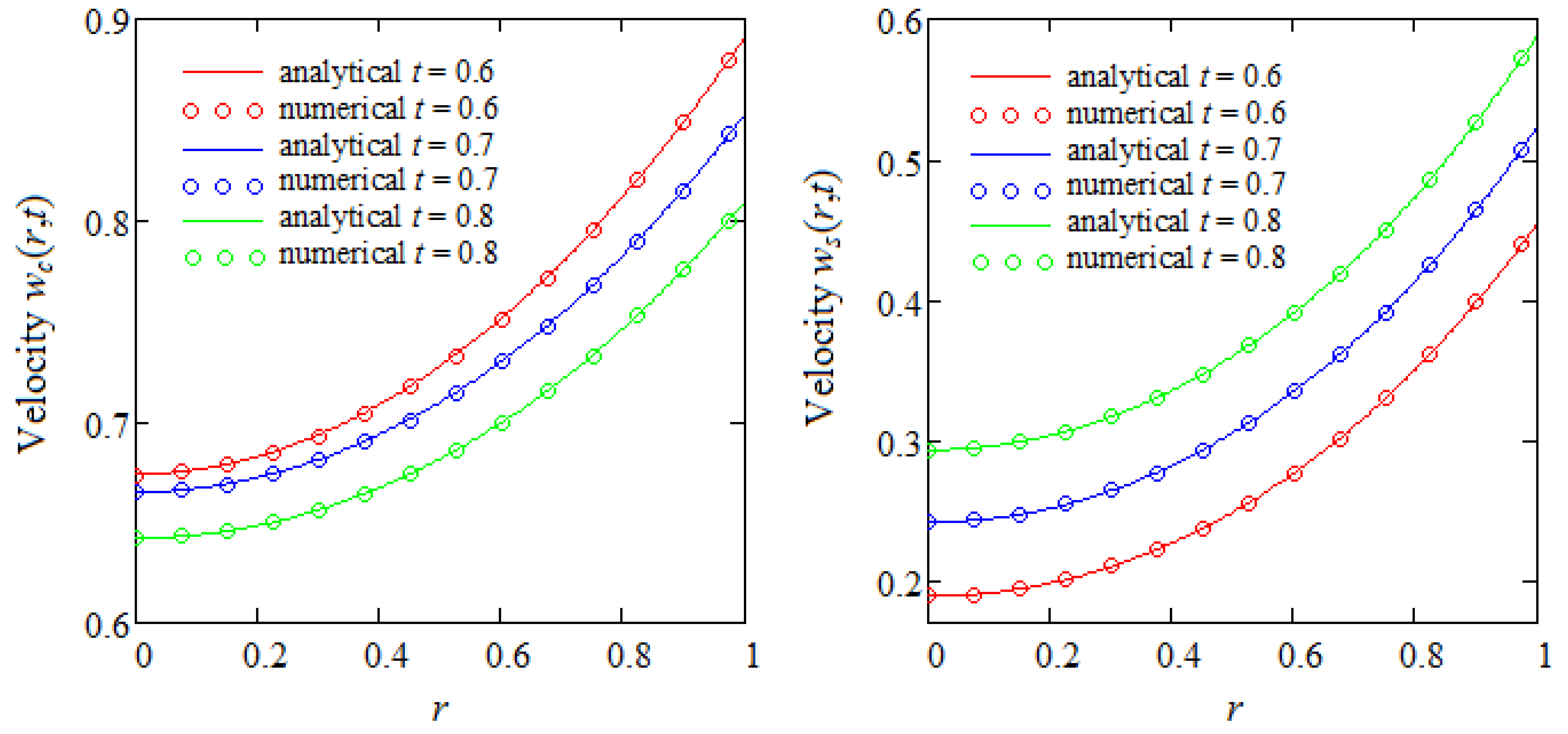
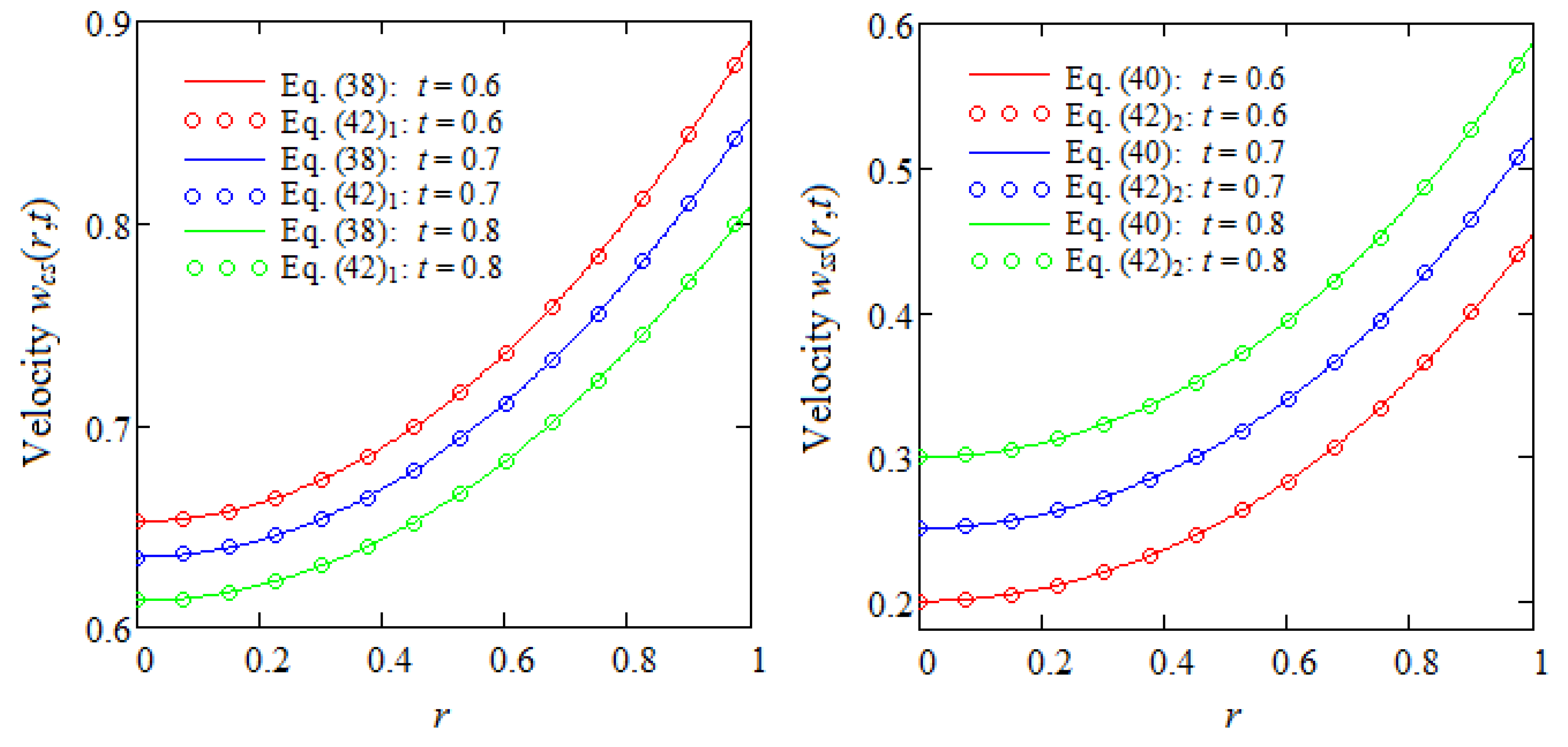
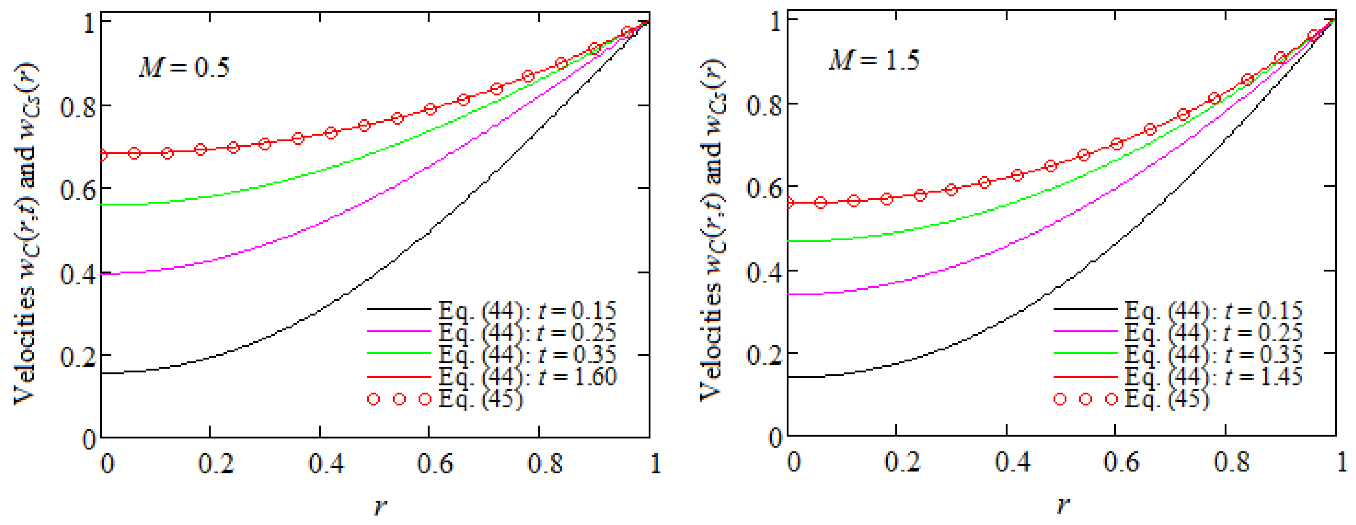
A general expression has been determined for velocity field, and certain special cases are considered for illustration. The results are validated and graphically proved using comparisons.

-

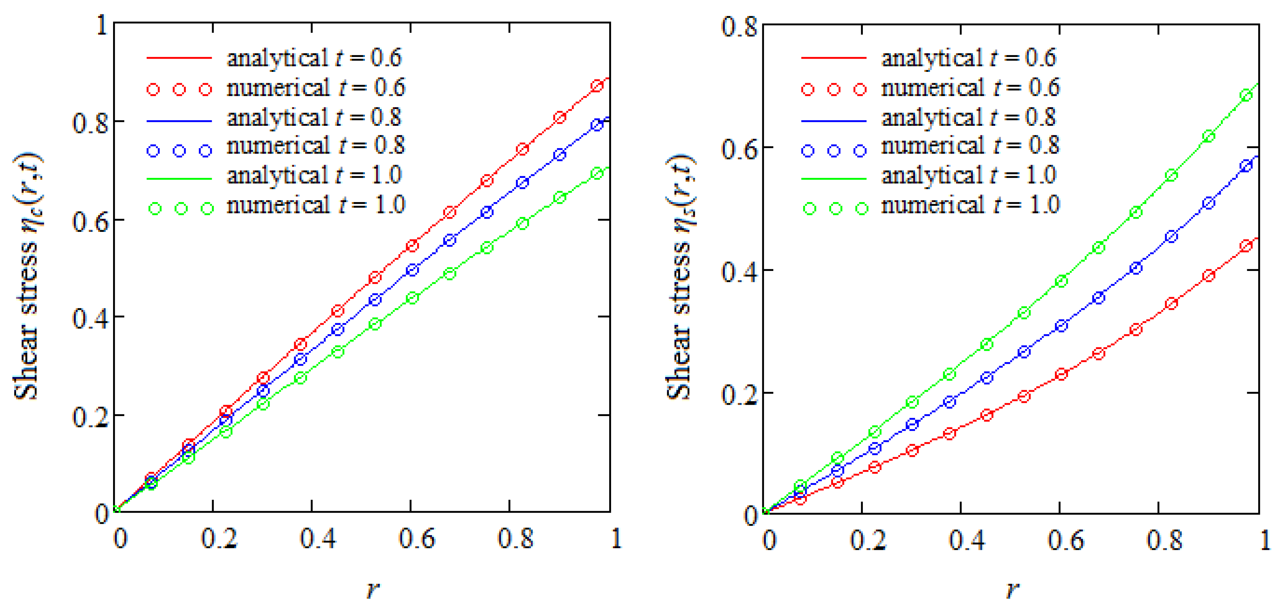
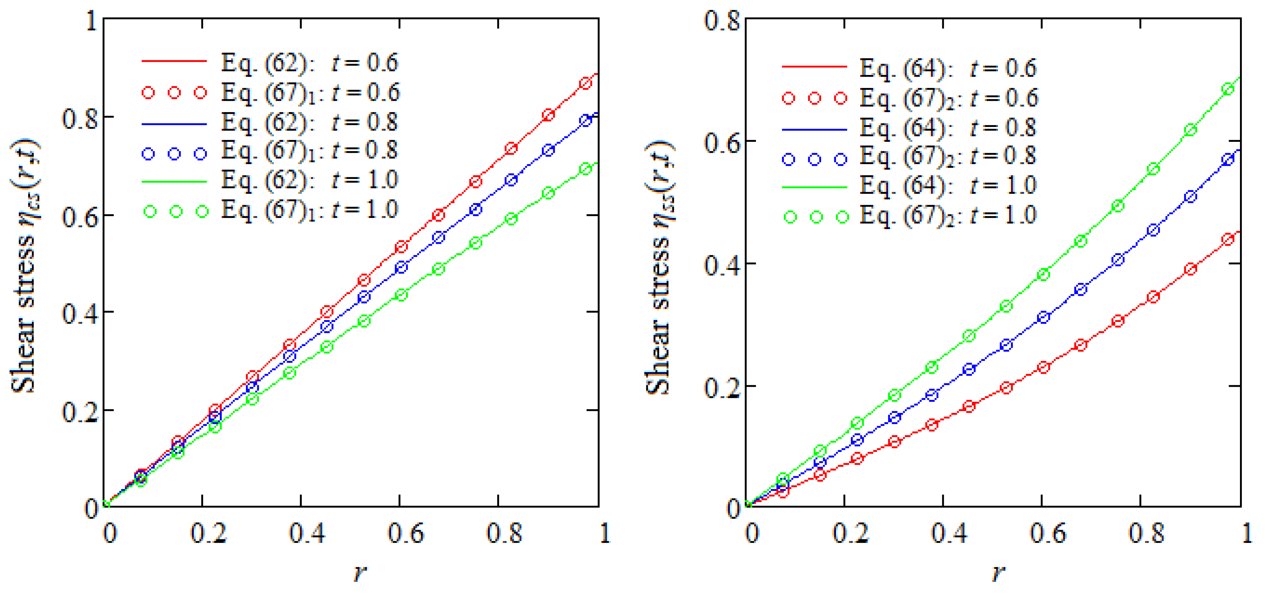
A governing equation for the non-trivial shear stress corresponding to the MHD unsteady motions of ECIOBFs in cylindrical domains is revealed for the first time.

-

This equation and the previous results allow us to easily find a general expression of shear stress for motions induced by a cylinder that applies an arbitrary shear to the fluid. The corresponding velocity can be obtained by solving the linear differential equation.

-

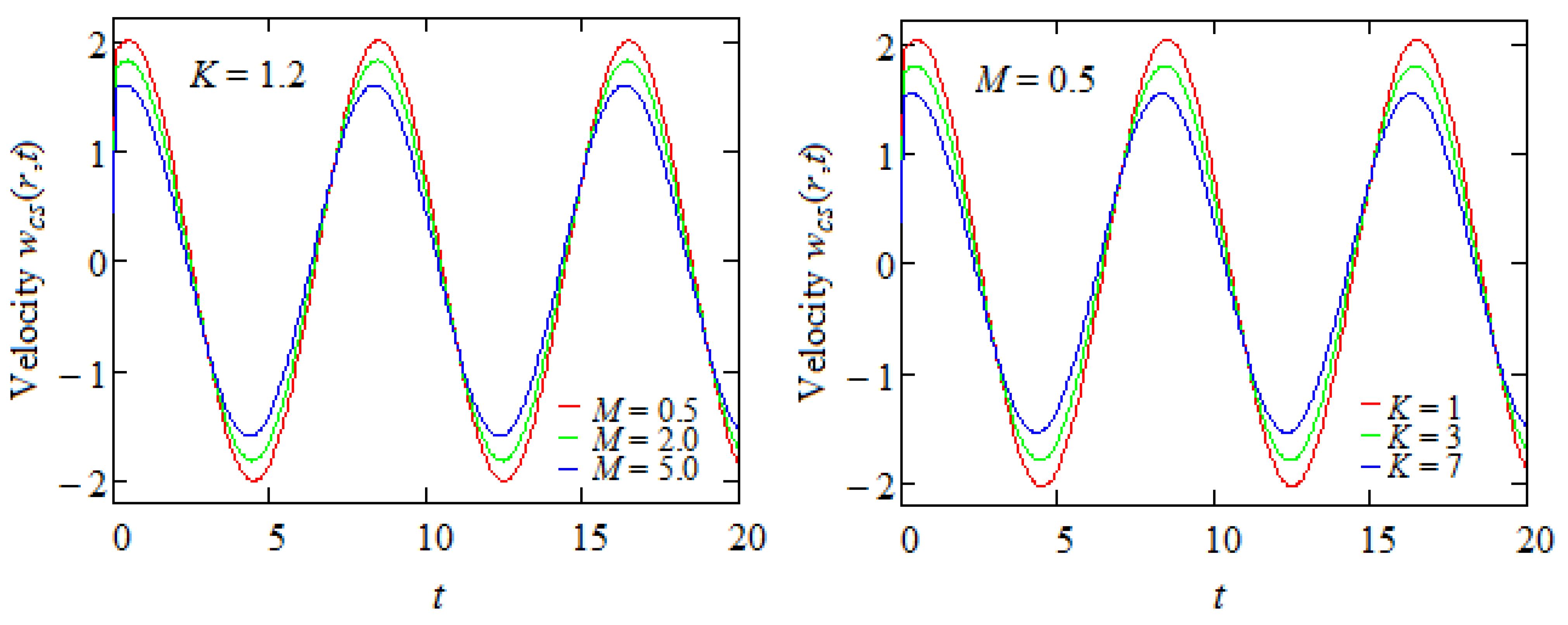
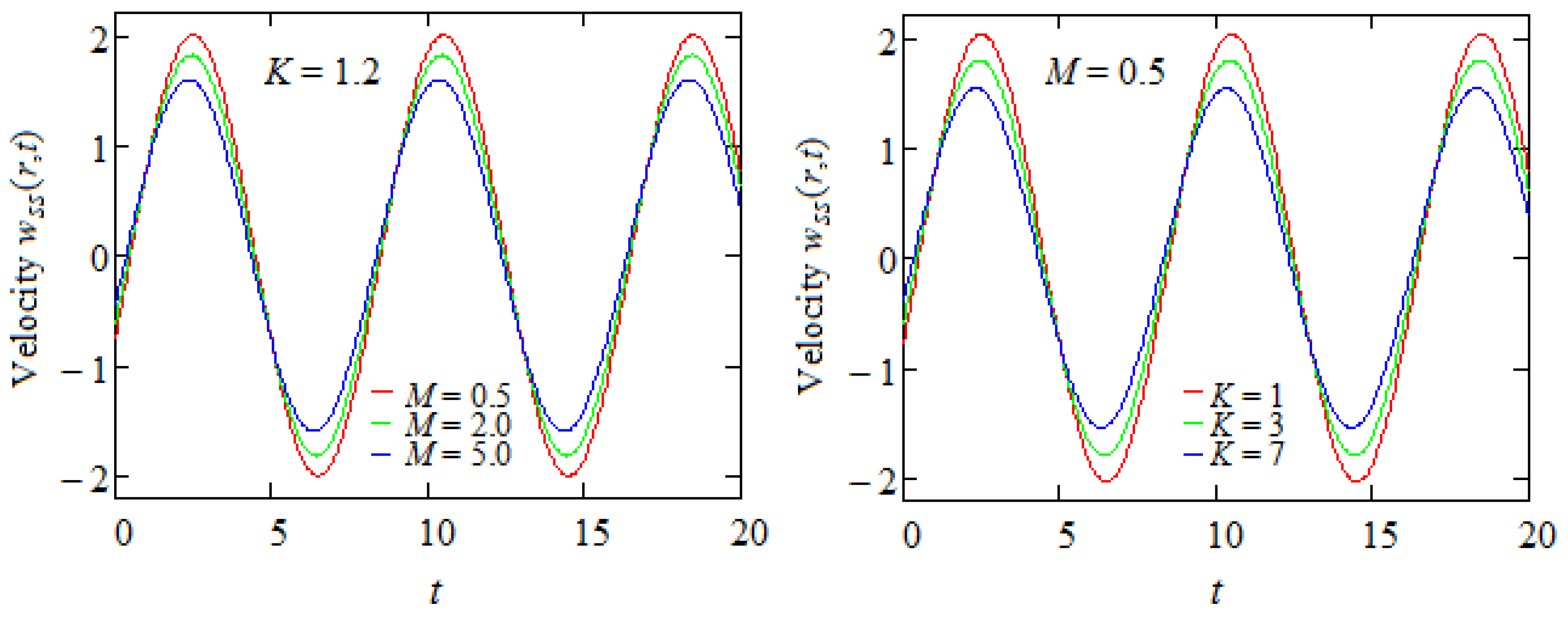
Graphical representations show that in the presence of a magnetic field or porous medium, as expected, the fluid moves more slowly and the steady state is reached earlier.

References

1. Oldroyd, J.G. On the formulation of rheological equations of state. Proc. R. Soc. Lond. Ser. A 1950, 200, 523–541. [Google Scholar] [CrossRef]
2. Bohme, G. Stromungsmechanik Nicht-Newtonscher Fluide; Teubner, B.G., Ed.; Springer: Stuttgart/Leipzig/Wiesbaden, Duitsland, 2000. [Google Scholar]
3. Waters, N.D.; King, M.J. The unsteady flow of an elastico-viscous liquid in a straight pipe of circular cross section. J. Phys. D Appl. Phys. 1971, 4, 204–211. [Google Scholar] [CrossRef]
4. Rajagopal, K.R.; Bhatnagar, R.K. Exact solutions for some simple flows of an Oldroyd-B fluid. Acta Mech. 1995, 113, 233–239. [Google Scholar] [CrossRef]
5. Wood, W.P. Transient viscoelastic helical flow in pipes of circular and annular cross-section. J. Non-Newton. Fluid Mech. 2001, 100, 115–126. [Google Scholar] [CrossRef]
6. Fetecau, C. Analytical solutions for non-Newtonian fluid flows in pipe-like domains. Int. J. Non-Linear Mech. 2004, 39, 225–231. [Google Scholar] [CrossRef]
7. Fetecau, C.; Fetecau, C.; Vieru, D. On some helical flows of Oldroyd-B fluids. Acta Mech. 2007, 189, 53–63. [Google Scholar] [CrossRef]
8. McGinty, S.; McKee, S.; McDermott, R. Analytic solutions of Newtonian and non-Newtonian pipe flows subject to a general time-dependent pressure gradient. J. Non-Newton. Fluid Mech. 2009, 162, 54–77. [Google Scholar] [CrossRef]
9. Khan, I.; Fakhar, K.; Anwar, M.I. Hydromagnetic rotating flows of an Oldroyd-B fluid in a porous medium. Spec. Top. Rev. Porous Media Int. J. 2012, 3, 89–95. [Google Scholar] [CrossRef]
10. Imran, M.; Tahir, M.; Imran, M.A.; Awan, A.U. Taylor-Couette flow of an Oldroyd-B fluid in an annulus subject to a time-dependent rotation. Am. J. Appl. Math. 2015, 3, 25–31. [Google Scholar] [CrossRef]
11. Ullah, S.; Tanveer, M.; Bajwa, S. Study of velocity and shear stress for unsteady flow of incompressible Oldroyd-B fluid between two concentric rotating circular cylinders. Hacet. J. Math. Stat. 2019, 48, 372–383. [Google Scholar] [CrossRef]
12. Tao, L.N. Magneto hydrodynamic effects on the formation of Couette flow. J. Aerospace Sci. 1960, 27, 334–338. [Google Scholar] [CrossRef]
13. Katagiri, M. Flow formation in Couette motion in magneto hydrodynamics. Phys. Soc. Jpn. 1962, 17, 393–396. [Google Scholar] [CrossRef]
14. Zahid, M.; Rana, M.A.; Haroom, T.; Siddiqui, A.M. Applications of Sumudu transform to MHD flows of an Oldroyd-B fluid. Appl. Math. Sci. 2013, 7, 7027–7036. [Google Scholar] [CrossRef]
15. Ghos, A.K.; Datta, S.K.; Sen, P. On hydromagnetic flow of an Oldroyd-B fluid between two oscillating plates. Int. J. Appl. Comput. Math. 2016, 2, 365–386. [Google Scholar] [CrossRef]
16. Hayat, T.; Hutter, K.; Asghar, S.; Siddiqui, A.M. MHD Flows of an Oldroyd-B Fluid. Math. Comput. Model. 2002, 36, 987–995. [Google Scholar] [CrossRef]
17. Hayat, T.; Hussain, M.; Khan, M. Hall effect on flows of an Oldroyd-B fluid through porous medium for cylindrical geometries. Comput. Math. Appl. 2006, 52, 269–282. [Google Scholar] [CrossRef]
18. Hamza, S.E.E. MHD flow of an Oldroyd-B fluid through porous medium in a circular channel under the effect of time dependent pressure gradient. Am. J. Fluid Dyn. 2017, 7, 1–11. [Google Scholar] [CrossRef]
19. Mohammed, G.G.; Salih, A.W. Impacts of porous medium on unsteady helical flows of generalized Oldroyd-B fluid with two infinite coaxial circular cylinders. Iraqi J. Sci. 2021, 62, 1686–1694. [Google Scholar] [CrossRef]
20. Ahadi, F.; Biglari, M.; Azadi, M.; Bodaghi, M. Computational fluid dynamics of coronary arteries with implanted stents: Effects of newtonian and non-newtonian blood flows. Eng. Rep. 2024, 6, e12779. [Google Scholar] [CrossRef]
21. Rossow, V.J. On flow of electrically conducting fluids over a flat plate in the presence of a transverse magnetic field. NACA TN Tech. Rep. 1957, 3971, 489–508. [Google Scholar]
22. Sneddon, I.N. Functional Analysis. In Encyclopedia of Physics/Handbuch der Physik; Flügge, S., Ed.; Springer: Berlin/Göttingen/Heidelberg, Germany, 1955; Volume 1/2. [Google Scholar] [CrossRef]
Figure 1. Comparison between numerical and analytical solutions w c ( r , t ) and w s ( r , t ) given by Equation (37) for α = 0.3 ,   β = 0.2 ,   ω = π / 4 ,   M = 0.5 ,   K = 1.2 , and three values of t.
Processes 12 01354 g001
Figure 2. Equivalence of the expressions of w c s ( r , t ) and w s s ( r , t ) given by Equations (38), (42)1 and (40), (42)2, respectively: α = 0.3 ,   β = 0.2 ,   ω = π / 4 ,   M = 0.5 ,   K = 1.2 , and three values of t.
Processes 12 01354 g002
Figure 3. Comparison between numerical and analytical solutions η c ( r , t ) and η s ( r , t ) given by Equation (61) for α = 0.3 ,   β = 0.2 ,   ω = π / 4 ,   M = 0.5 , and three values of t.
Processes 12 01354 g003
Figure 4. Equivalence of the expressions of η c s ( r , t ) and η s s ( r , t ) given by Equations (62), (67)1 and (64), (67)2, respectively, for α = 0.3 ,   β = 0.2 ,   ω = π / 2 ,   M = 0.25 , and three values of t.
Processes 12 01354 g004
Figure 5. Convergence of starting velocity w C ( r , t ) , given by Equation (44), to its steady component w C s ( r ) , given by Equation (45), for α = 0.3 ,   β = 0.2 ,   K = 1.2 ,   M = 0.5 , or M = 1.5 and increasing values of t.
Processes 12 01354 g005
Figure 6. Convergence of starting velocity w C ( r , t ) , given by Equation (44), to its steady component w C s ( r ) , given by Equation (45), for α = 0.3 ,   β = 0.2 ,   M = 0.8 ,   K = 1.5 or K = 3 and increasing values of t.
Processes 12 01354 g006
Figure 7. Variations in time of velocity w c s ( r , t ) , given by Equation (38), for α = 0.3 ,   β = 0.2 ,   ω = π / 4 ,   r = 1 / 2 ,   K = 1.2 , and increasing values of M, M = 0.5 , and increasing values of K.
Processes 12 01354 g007
Figure 8. Variations in time of velocity w s s ( r , t ) , given by Equation (40), for α = 0.3 ,   β = 0.2 ,   ω = π / 4 ,   r = 1 / 2 ,   K = 1.2 , and increasing values of M, M = 0.5 , and increasing values of K.
Processes 12 01354 g008