Abstract
Shear wave velocity is one of the important parameters reflecting the lithological and physical properties of reservoirs, and it is widely used in the fields of lithology and fluid property identification, reservoir evaluation, seismic data processing, and interpretation. However, due to the high cost and challenge of obtaining shear wave velocity, only a few key wells are measured. Considering the intricate nonlinear mapping relationship between shear wave velocity and conventional logging data, an integrated network incorporating an attention mechanism, a convolutional neural network, and a bidirectional gated recurrent unit (STACBiN) is proposed for predicting shear wave velocity. The impact of conventional logging data on shear wave velocity is analyzed, thus employing the attention mechanism to focus on data correlated with shear wave velocity, which can enable the prediction results of the method proposed superior to those of conventional methods. Additionally, the prediction results of this method are compared with the prediction results of the two-dimensional convolutional neural network (2DCNN) and bidirectional gated recurrent unit (BiGRU). It is verified that the network proposed can effectively predict the shear wave velocity, with minimal error between predicted and true values.
1. Introduction
The key task of successfully discovering oil and gas reservoirs is the prediction of elastic parameters in seismic exploration. Elastic parameters, such as compressional wave velocity (DTC) and shear wave velocity (DTS), are fundamental characteristics of seismic wave propagation in underground media. Their determination and interpretation are crucial for revealing underground structures, detecting the existence of oil and gas reservoirs, and assessing reserves. The variation in shear wave velocity can reflect the elastic properties of rocks, such as porosity, permeability, and the mineral composition of the rock matrix. Additionally, it can also reveal the underground stress state and fluid type. However, due to the constraints of acquisition costs and technology, shear wave velocity is commonly missing in some old wells. The experience equation and the petrophysical model were used to predict shear wave velocity [1,2,3,4]. For all complex geological conditions or special rock types, empirical formulas may not provide accurate predictions.
Due to the diversity of rock structure characteristics of various reservoirs, the establishment of targeted rock physics models based on the concept of equivalent media has been a subject of research for scholars both domestically and abroad. The influence of shale content, porosity, and pore shape on rock velocities in shaly sandstone was considered by Xu and White [5], and a classical Xu–White model was proposed to describe the elastic properties of sandstone. The calculation methods for the bulk and shear moduli of dry rock in the Xu–White model for shear wave velocity prediction were simplified by Keys and Xu [6], which can significantly enhance the computational efficiency of the Xu–White model. When constructing models for carbonate reservoirs, the pores of carbonate rocks were categorized as clay-containing pores, intergranular pores, microfractures, and hard pores by Xu and Payne [7], thus extending the application of the Xu–White model to carbonate reservoirs. The Xu–White model was utilized for shear wave prediction, and the rock physics analysis, pre-stack elastic parameter inversion, and other techniques were combined to achieve reservoir prediction from point to plane by Liu et al. [8]. The predicted values exhibited a high degree of agreement with the true values. The variation in clay elastic parameters was considered by Zheng et al. [9], and the inversion was employed to correct errors in the input parameters of the Xu–White model, which can improve the prediction accuracy of shear wave velocity. A shear wave velocity model for porous fractured sandstone based on the Gassmann equation was established by Li et al. [10], and consolidation parameters proposed by Lee were utilized to calculate the shear wave velocity. The results based on the DEM-Gassmann rock physics model were optimized by Yang et al. [11] using simulated annealing, and the virtual fracture porosity was utilized to make up for the error caused by the inaccuracy of rock elastic parameters and physical parameters. A porosity aspect ratio estimation method based on a rock physics model was proposed by Guo et al. [12], whereby the aspect ratio of pores is estimated using compressional wave velocity, porosity, and mineral composition, thus predicting shear wave velocity. The microstructure of shale reservoirs was described by Zhang and Liu [13] using a fracture aspect ratio and compaction index, and a quantitative relationship between the petrophysical parameters and elastic parameters of shale reservoirs was established using statistical rock physics models. The above rock physics model method usually involves complex rock mechanics theory and numerical simulation, which requires a lot of computing resources and time, as well as a large number of rock parameters as input. These parameters may be difficult to obtain or measure accurately [14]. Therefore, finding a reliable and adaptable method for predicting shear wave velocity has always been a focus of research.
With the continuous development of computers, neural networks capable of extracting data features and constructing complex nonlinear mapping relationships have been widely used in various fields such as image processing, medical health, and autonomous driving [15,16,17]. In recent years, neural networks capable of establishing complex nonlinear mapping relationships between input and output, such as convolutional neural networks (CNNs) [18], recurrent neural networks (RNNs) [19], and generative adversarial networks (GANs) [20], have been introduced into the field of geophysics by some scholars, achieving partial success in reservoir prediction, lithology identification, and stress analysis [21,22,23]. The application of adaptive BP neural networks in shear wave velocity prediction was proposed by Wang et al. [24]. The neural network model predicts that the shear wave velocity is in good agreement with the measured shear wave velocity. A convolutional neural network containing the receiving function was designed by Yang et al. [25] to predict the shear wave velocity. To fully consider the inherent relationship between shear wave velocity and other logging data, a one-dimensional convolutional neural network was used to predict shear wave velocity by Ma et al. [26]. Due to the gradual variation of sedimentary formation, logging data exhibits a correlation in the depth direction. RNNs have been used to extract temporal features among conventional logging data, successfully predicting reservoir parameters and formation pressure by some scholars [27,28]. The temporal features from logging data were extracted for predicting shear wave velocity by Sun et al. [29] using GRU. A GRU was employed to reconstruct the logarithmic curve by Teng et al. [30]. Compared with long short-term memory (LSTM), GRUs have a significant improvement in the average correlation coefficient of prediction results. However, the above methods did not fully consider the spatiotemporal features of logging data, which may limit the accuracy and reliability of neural network prediction results. Therefore, some scholars adopt network fusion or incorporate attention mechanisms to improve the prediction accuracy of neural networks [31]. The spatial and temporal features of the logging data were extracted by Wang et al. [32] using CNNs and GRUs, respectively, and the relationship between different spatial and temporal features and shear wave velocity was established. Compared with the prediction results of traditional networks, the prediction results of the network proposed are closer to the true values. The spatiotemporal features of logging data were extracted using 2DCNNs and GRUs by Chen et al. [21]. Compared with the prediction results of traditional networks, it can be observed that the network proposed can effectively fit the shear wave velocity in sandstone sections. Aiming at the nonlinear relationship between different logging data, a shear wave velocity prediction method based on an attention mechanism and a bidirectional long short-term memory network was proposed by He et al. [33]. To reduce the deviation of underground oil and gas distribution description, an attention mechanism is integrated into the long-term and short-term memory networks to automatically calculate the weight of data features, and the shear wave velocity is predicted by Fu et al. [34] with a lower mean absolute error. To improve the prediction accuracy of porosity, the method of combining bidirectional long short-term memory networks and attention mechanisms was proposed by Qiao et al. [35], and it is verified that the proposed network has the smallest training error on the verification set. Aiming at the problems of gradient explosion and gradient disappearance of traditional recurrent neural networks (RNNs), a new network that is sensitive to the depth sequence of logging data was proposed by Feng et al. [36]. The attention mechanism is fused with BiLSTM to highlight the temporal features that are important for shear wave velocity, reduce the influence of other features, and then improve the prediction accuracy of shear wave velocity. The attention mechanism of the network was utilized to allocate weights to logging data, automatically focusing on the logging data that contribute greatly to the shear wave velocity prediction, thus significantly improving the prediction accuracy.
Shear wave velocity is one of the key parameters of rock physical properties. It is closely related to various characteristics of underground rock, including rock density, porosity, fluid type, and mechanical properties of rock. However, due to the high cost of obtaining shear wave velocity, shear wave velocity is generally lacking in actual data. Aiming at the problem that the traditional network is not sensitive to the spatiotemporal features of logging data and that the accuracy of shear wave velocity prediction is low, an integrated network based on an attention mechanism (STACBiN) is proposed. The spatial and temporal features of logging data are extracted using a convolutional neural network and bidirectional gated recurrent unit, respectively. Simultaneously, under the influence of the spatiotemporal attention mechanism, different spatiotemporal features are assigned different weights, thereby enhancing the overall performance and prediction accuracy of the network proposed. Finally, the stratum of a basin offshore is taken as the research object, and the prediction results of the STACBiN integrated network are compared with the prediction results of the traditional convolutional neural network (2DCNN) and the bidirectional gated recurrent unit (BiGRU) to verify the effectiveness of the proposed method.
2. Methods
2.1. Convolutional Neural Network (CNN)
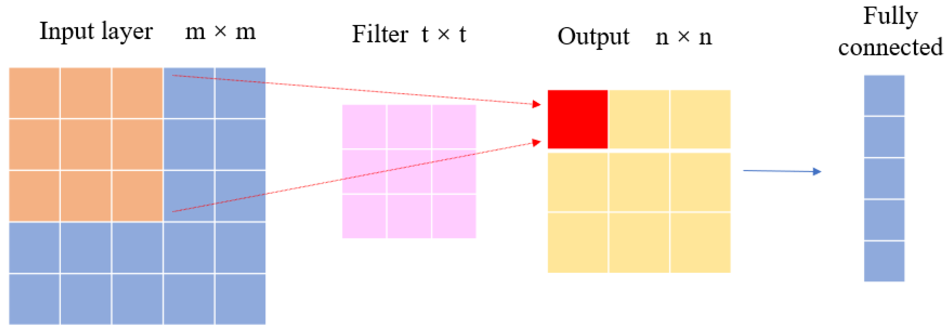
A convolutional neural network (CNN) is a type of deep learning network that is mainly composed of an input layer, convolutional layer, fully connected layer, and output layer (Figure 1). The convolutional layer is the core component of a CNN, composed of a series of filters (also known as convolutional kernels). When the input data are input into the convolutional neural network, the filter performs a convolution operation with the input data to extract the spatial features.

Figure 1.
Structure of CNN.
2.2. Bidirectional Gated Recurrent Unit (BiGRU)
A gated recurrent unit (GRU) that addresses the problems of vanishing and exploding gradients [37] is a variant of an RNN. It replaces the input gate, forget gate, and output gate of the LSTM with a reset gate and update gate, thereby optimizing the internal structure of the unit and improving the computational efficiency.
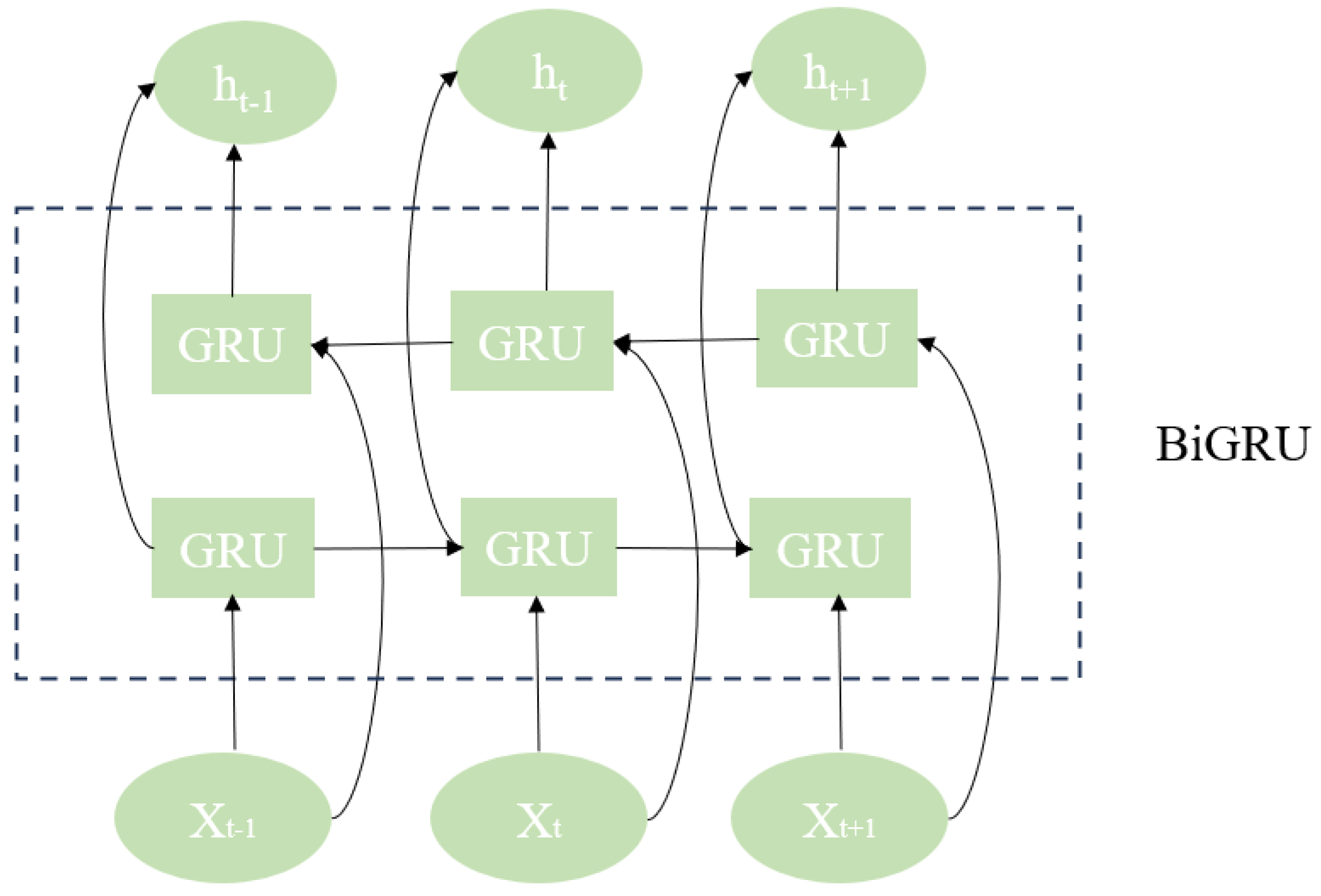
The bidirectional gated recurrent unit network (BiGRU) combines two independent units (Figure 2). One deals with the input sequence in chronological order, and the other deals with the input sequence in the opposite order, so that the model can fully consider the past and present influencing factors, capture the information in the input sequence more comprehensively, and improve the expression ability of the model.
where and represent the hidden states from left to right and from right to left, respectively. GRU represents the GRU unit and represents the t-th element of the input sequence. Then, the forward and reverse hidden states are spliced to obtain the final hidden state . Finally, the is passed to a fully connected layer, and the output is obtained using the softmax function.
where and represent the weight and bias of the fully connected layer, respectively; “” represents an activation function; and “[]” represents that the two hidden states are spliced.
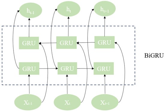
Figure 2.
Structure of BiGRU.
2.3. Temporal Attention Mechanism
The design of the attention mechanism is inspired by human research on the visual system. Its principle is to allow people to focus more attention on important areas, suppressing other irrelevant information, and thereby obtaining more useful information. The temporal attention mechanism is a type of attention mechanism that primarily allocates different weights to different temporal features, thereby enhancing the model’s response to important temporal features. Although the BiGRU is used to extract different temporal features of data, it cannot highlight the influence of important temporal features on labels, thus affecting the prediction effect of the neural network. Therefore, the temporal attention mechanism is integrated with the bidirectional gated recurrent unit to solve the above problems.
In the field of geophysics, due to the gradual variation of sedimentary strata, the logging data are correlated in sequence direction. Assuming that the temporal features can be expressed as , t represents the length of the temporal features and n represents the dimensionality of each feature in each time step. Under the effect of the temporal attention mechanism, the final output can be represented as
where represents the weight coefficients assigned by the temporal attention layer for different temporal features. “” is a normalization function that can map the weights to the range [0, 1]. and represent the weight matrix and bias, respectively. “” represents the dot product operation between vectors. is the result of temporal attention layer weighting.
2.4. Spatial Attention Mechanism
Conventional logging data have different correlations with shear wave velocity. Therefore, the correlations between different spatial features extracted through convolutional neural networks and shear wave velocity are also different. However, traditional CNNs assign irregular weights to different spatial features extracted, which cannot highlight the influence of important spatial features on the label. Therefore, the spatial attention mechanism is integrated with the convolutional neural network. Assuming that the spatial features can be expressed as , t represents the t-th spatial feature extracted by the t-th convolutional kernel and n represents the number of channels in the kernel. Under the effect of the spatial attention mechanism, the output of can be represented as
where represents the weight coefficients assigned by the spatial attention layer for different spatial features. and are the weight and bias, respectively. is the calculation result of spatial attention layer weighting.
2.5. STACBiN Integrated Network Structure
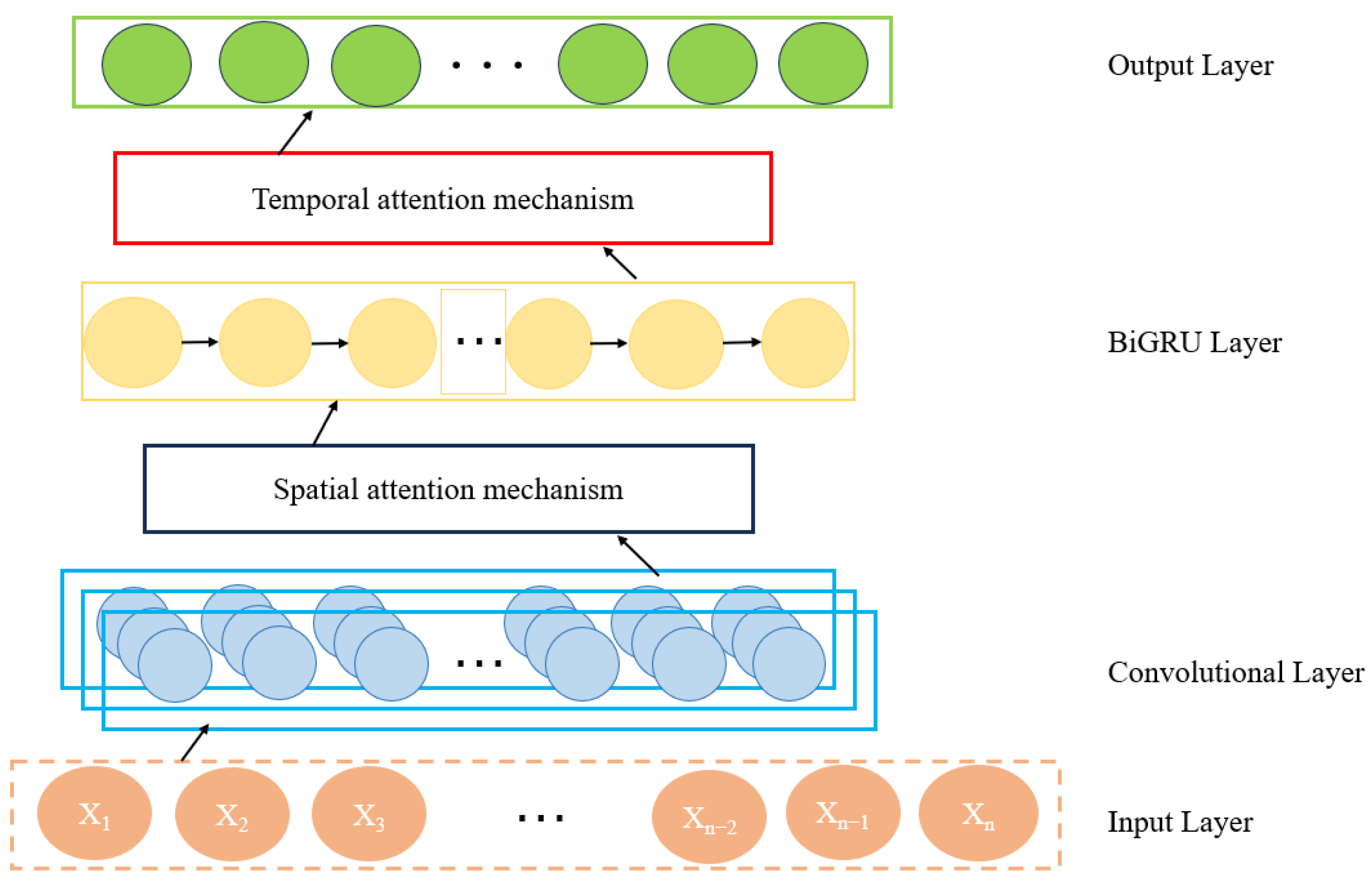
In the field of geophysics, logging data are usually obtained during drilling and are often used to measure the properties of underground rocks. Due to the complexity of stratigraphic geology, the interface between different strata may be blurred, which increases the complexity of shear wave velocity prediction. To solve the problems, an integrated network based on the attention mechanism (STACBiN) is presented (Figure 3), which consists of the 2D convolutional layers, the spatial attention layer, the bidirectional gated recurrent units, the temporal attention layer, and the fully connected layer (FNN). The temporal and local spatial features between multi-dimensional logging data can be extracted using BiGRU and 2DCNN and assigned different weights under the action of spatiotemporal attention mechanism, so as to improve the overall performance and prediction effect of the network. Finally, data fitting is carried out under the action of a fully connected layer, so as to establish a complex nonlinear mapping relationship between other logging data and shear wave velocity.

Figure 3.
Structure of STACBiN integrated network.
3. Experimental Procedure and Operations
3.1. Training and Prediction Process of STACBiN Integrated Network
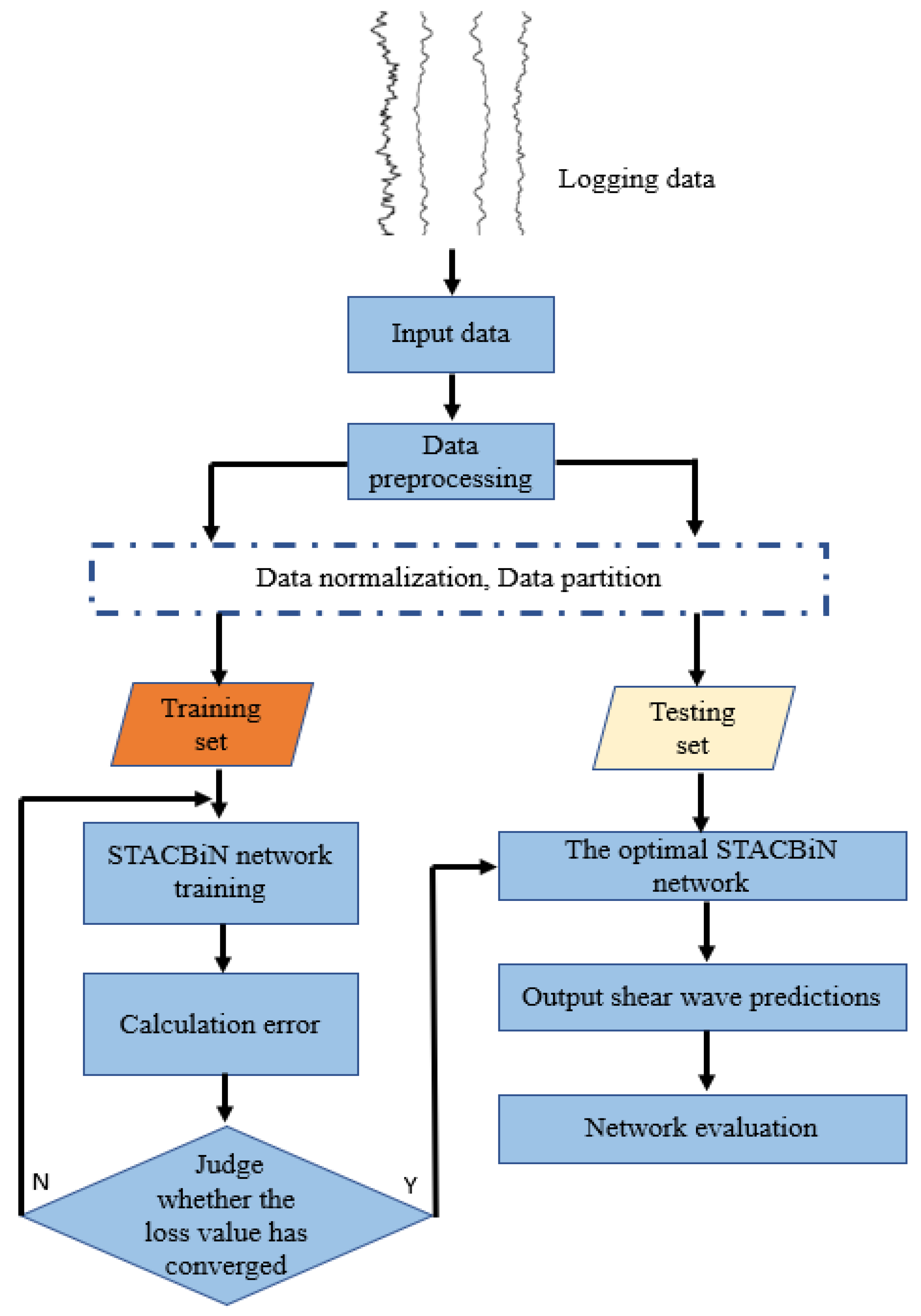
The process of shear wave velocity prediction using a STACBiN integrated network is as follows (Figure 4):

Figure 4.
The training and prediction process of STACBiN integrated network.
(1) Feature Selection. Conduct a correlation analysis between shear wave velocity and other logging data using scatter plots and select the well data that hold a high correlation with shear wave velocity as inputs for the neural network.
(2) Data Preprocessing. To eliminate differences in scale among different logging data and improve computational efficiency, a normalization function is used:
where represents the logging data. and are the minimum and maximum values of the logging data, respectively, and is the normalized value.
(3) Network Training. The preprocessed data are divided into training and testing sets. The training set is input into the neural network for training. The mean square error (MSE) is used as the loss function of the network to calculate the error. In addition, the adaptive moment estimation (Adam) [38,39] is used as an optimization algorithm to update the network parameters until the loss error converges and remains unchanged.
where is the number of training samples, is the predicted value, and is the true value.
(4) Input Testing Data. The divided test set is input into the optimal network for shear wave velocity prediction.
(5) Model Evaluation. The mean absolute error (MAE) and coefficient of determination (R2) are used as evaluation indices to quantitatively evaluate the neural network. The closer the mean absolute error is to 0, the closer the predicted values are to the true values. The closer the coefficient of determination is to 1, the closer the predicted values are to the true values.
where is the number of samples, is the mean of the training samples, is the i-th input sample data, and is the output of the network.
3.2. Dataset Introduction
The dataset in this paper is derived from the sand–mudstone strata of an offshore basin. The depth of the target layer is mainly composed of sandstone and mudstone. In order to improve the prediction accuracy of shear wave velocity in tight sandstone reservoirs, an integrated network combined with attention mechanisms is proposed. There are eight measured wells in this area, of which five wells involve shear wave velocity, which are labeled as FH-1, FH-2, FH-3, FH-4, and FH-5, respectively. Among these, the FH-1, FH-2, and FH-3 wells are utilized as the training set to train the network, while the FH-4 and FH-5 wells are used as the test set to validate the generalization of the network.
3.3. Feature Selection
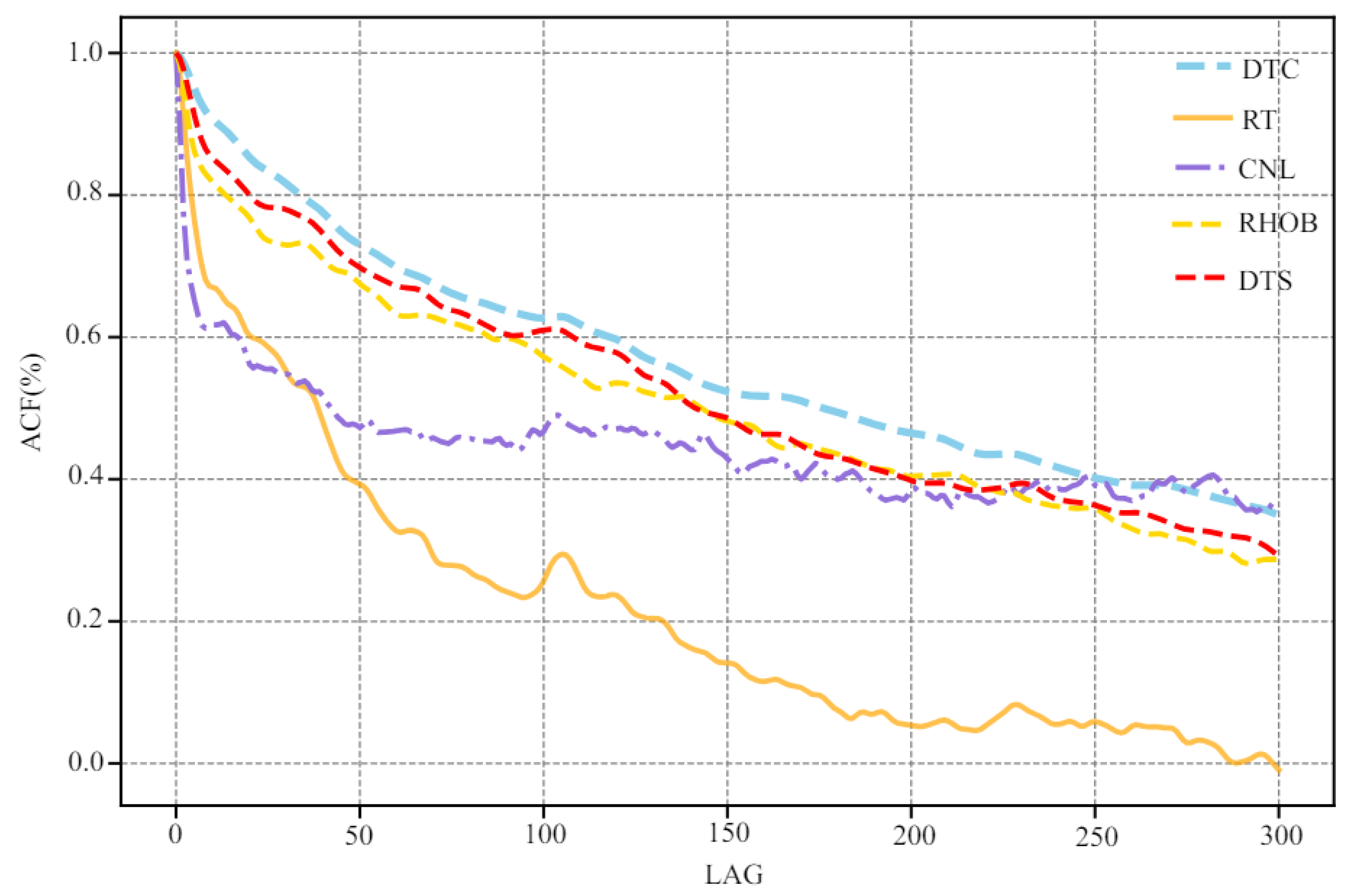
In essence, using deep learning to predict shear wave velocity is a data fitting problem. Therefore, the accuracy of the prediction results mainly relies on the correlation between the input and the output. The density, compensated neutron, resistivity, and compressional wave velocity in all wells are selected as the input of the neural network. Figure 5 shows the correlations between logging data and shear wave velocity, and the correlations are as follows: compression wave velocity (DTC, R = 0.85), resistivity (RT, R = −0.73), density (RHOB, R = −0.70), and compensated neutron (CNL, R = 0.63). The DTC and CNL are positively correlated with the shear wave velocity, and the RHOB and RT are negatively correlated with the shear wave velocity. On the other hand, due to the correlation of sedimentary strata in the depth direction, the logging data have regularity in the sequence direction. Therefore, the autocorrelation algorithm is used to interpret the self-relativity of logging data (Figure 6). It can be seen that with the increase in lag moment (LAG), the degree of autocorrelation reduction in different logging data is different. When the lag is 100, the autocorrelation of logging data from high to low is DTC, DTS, RHOB, CNL, and RT. This analysis shows that there are different correlations between different spatial and temporal features of other logging data and DTS.
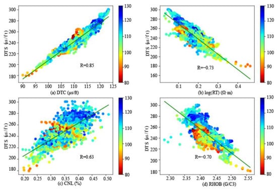
Figure 5.
Correlation analysis of different logging data and shear wave velocity (a) DTS-DTC. (b) DTS-RT. (c) DTS-CNL. (d) DTS-RHOB. (R is the Pearson coefficient.)
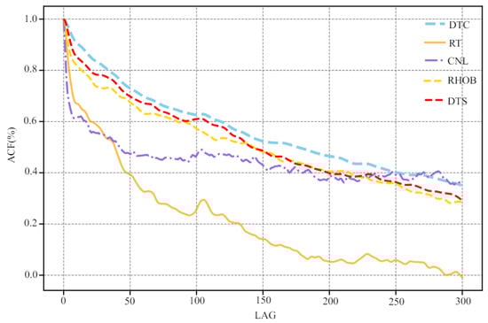
Figure 6.
Autocorrelation of conventional logging data.
3.4. Selection of Hyperparameters
Since the convolutional neural network was originally applied to the field of image classification, the recurrent neural network was initially successfully applied to the field of natural language processing. It has relatively few applications in the field of geophysics, and there are many factors that affect the neural network, such as time step, learning rate, etc., so it is necessary to analyze each parameter. Therefore, it is necessary to conduct sensitive parameter experiments on the network proposed in this paper and use the coefficient of determination (R2) to quantitatively evaluate the superiority of various parameter settings, so as to obtain the best hyperparameters for the basic parameter settings of the network.
The most important parameters in the neural network are the number of neurons and the number of layers, which together determine the complexity and learning ability of the network. The number of nodes and layers of the hidden layer has a significant impact on network performance, but it is not simply considered that the more layers, the better. In fact, although increasing the number of hidden layers can improve the expression ability of the network and enable it to learn more complex nonlinear mappings, it may also bring some problems, such as overfitting. Moreover, more hidden layers may cause problems such as gradient disappearance or explosion in the error backpropagation process of the neural network, thereby increasing the training difficulty of the network. The number of neurons in the neural network also follows this rule. Therefore, the determination of the hyperparameters in the neural network needs to be confirmed one by one through a specific scenario to determine the optimal neural network parameters in a specific scenario. In addition to the parameters such as the hidden layer of the neural network and the number of neurons, the parameters of the network proposed mainly include the time step (sliding window) and learning rate. The time step represents the corresponding relationship between the multi-point and single-point shear wave velocity in other logging data. When strata change or lithology difference is obvious, the change point can be selected as the division point of the time step, so as to establish a complex mapping relationship between logging data and shear wave velocity in each time step. The learning rate plays a crucial role in deep learning networks, which is a hyperparameter used to control the step size of the network parameters updated in each iteration. An improper learning rate may lead to problems such as unstable network training, slow convergence speed, or convergence to local optimal solutions. Therefore, the determination of learning rate needs to be tested repeatedly.
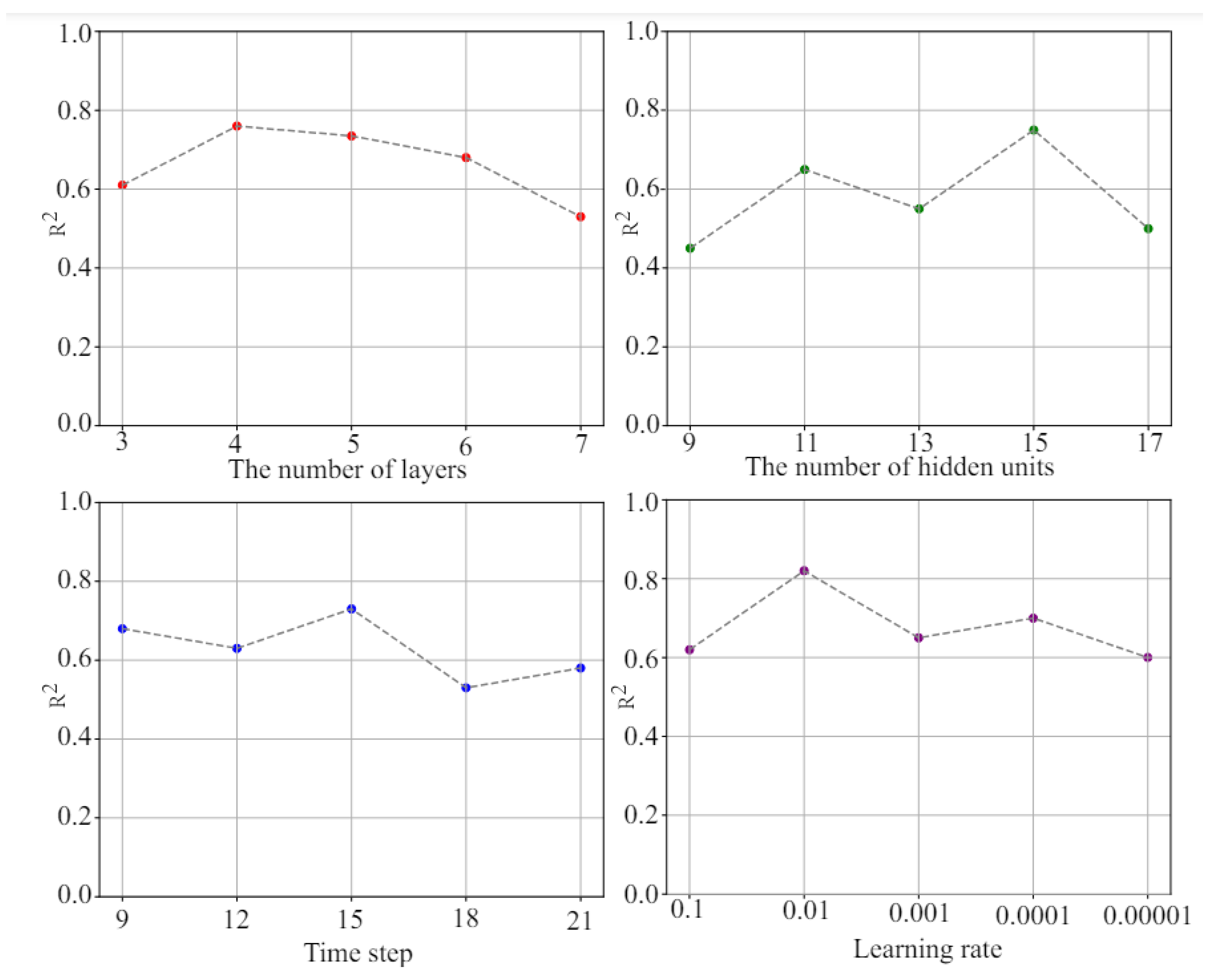
The FH-1, FH-2, and FH-3 wells are used as the training set and the FH-4 and FH-5 wells are used as the test set; by examining the performance of the STACBiN integrated network on the test set under different hyperparameters, the optimal network parameters are determined one by one. Finally, the hyperparameter combination with 4 hidden layers, 15 hidden units, 15 time steps, and a 0.01 learning rate is selected (Figure 7), and the network architecture is determined based on this experiment.
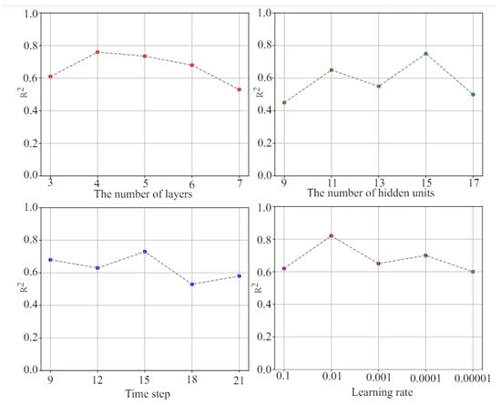
Figure 7.
The evaluation results of each parameter.
3.5. Visualization of Attention Weight
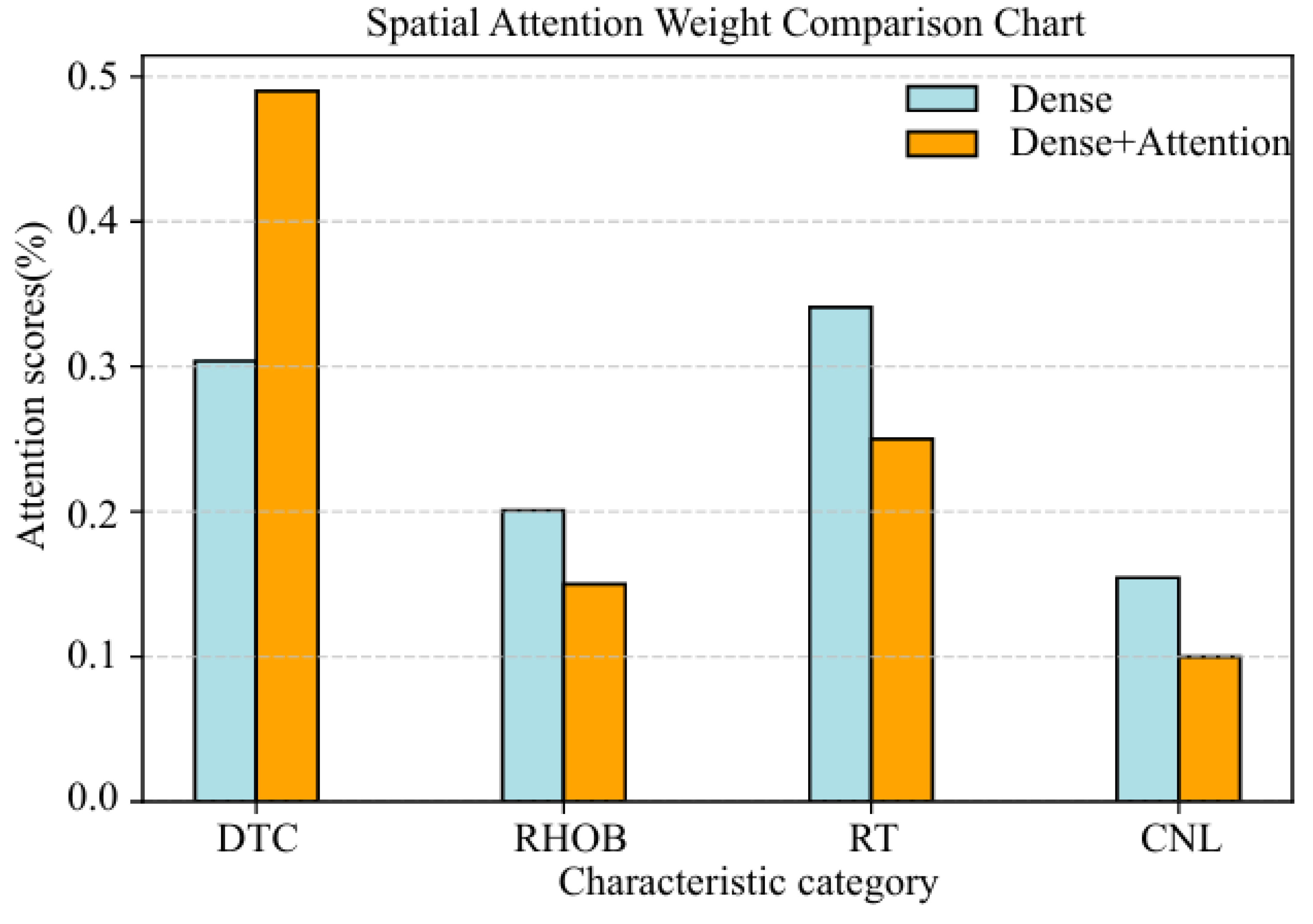
In order to verify the rationality of adding an attention mechanism to the neural network, two networks with and without spatiotemporal attention mechanisms are constructed, respectively. The structure of the network without a spatiotemporal attention mechanism is composed of a 2DCNN, a BiGRU, and a fully connected layer. Meanwhile, the structure of the network with a spatiotemporal attention mechanism is composed of a 2DCNN, a spatial attention layer, a BiGRU, a temporal attention layer, and a fully connected layer. Figure 8 demonstrates the weight distribution of the neural network with or without spatial attention layer. It can be clearly seen that the spatial attention layer assigns different weights to different logging data, from high to low: DTC, RT, RHOB, and CNL. The weight of DTC given by the spatial attention layer is the largest, reaching about 0.49, and the weight of CNL is the smallest, reaching about 0.10. This means that there is the largest correlation between DTC and DTS and the smallest correlation between CNL and DTS, which is consistent with the distribution of the Pearson correlation coefficient in Figure 5, which is consistent with the correlation distribution between conventional logging data and shear wave velocity in Figure 5. However, the weight distribution of the network without a spatial attention mechanism does not have this rule. This is because both DTS and DTC reflect the response of rock to stress. Under various geological conditions, the DTC and DTS of rocks are typically similarly influenced, showing a positive correlation between the two, which validates the reasonability of introducing the spatial attention mechanism.
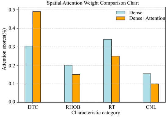
Figure 8.
Weight distribution with or without spatial attention layer.
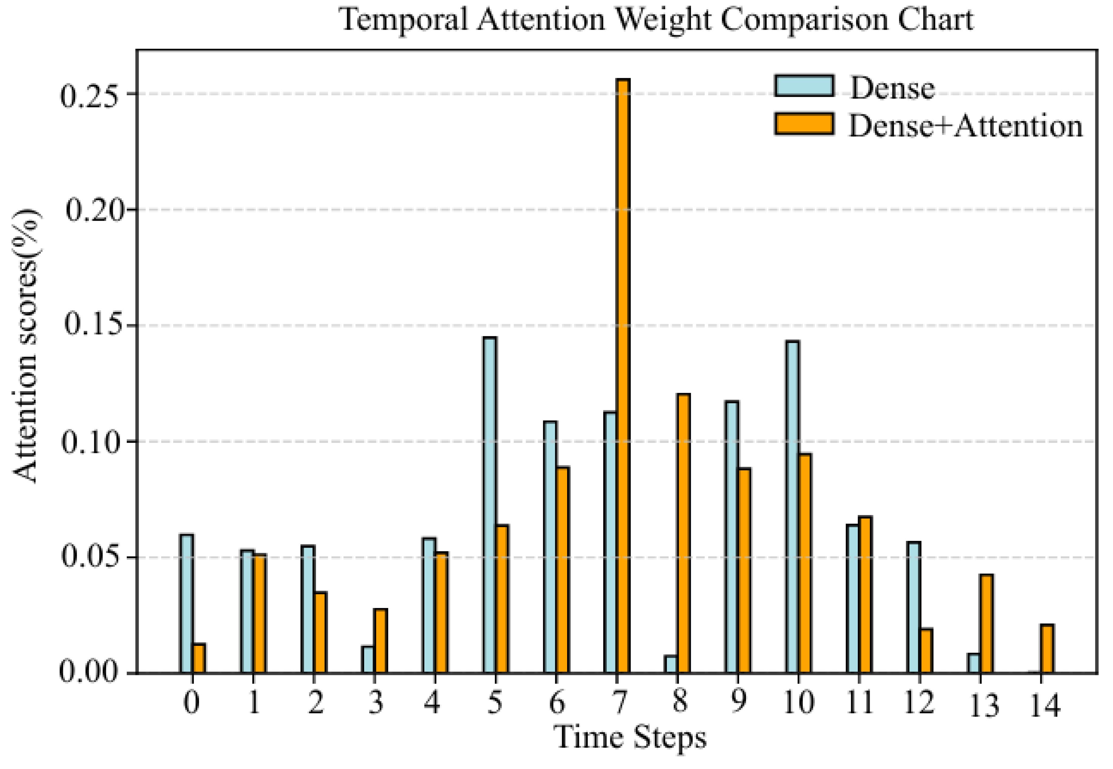
Figure 9 demonstrates the weight distribution of the neural network with or without the temporal attention layer. It can be observed that the temporal feature at the label position is given the largest weight, reaching 0.2561, indicating that the correlation between the temporal feature at this position has the greatest influence on the shear wave velocity. Secondly, with the increasing distance between the temporal feature and the temporal feature at the label, the weight assigned by the temporal attention mechanism shows a downward trend, which is consistent with the variation in conventional logging data with lag distance in Figure 6. This is because the label is located at the same position as the sampling point in the middle of the sample, which is the different response of the same rock, so the correlation is the largest. In addition, the sedimentary strata are gradually changing in the depth direction, and the logging data are correlated in the sequence direction. As the distance increases, the correlation gradually becomes smaller, so it proves to be reasonable.
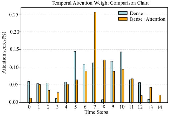
Figure 9.
Weight distribution with or without temporal attention layer.
4. Network Comparative Analysis
In order to verify the effectiveness of the network proposed in this paper, the prediction results of the network proposed are compared with the prediction results of the traditional 2DCNN and BiGRU. All networks use the Adam algorithm for parameter optimization, and these network structures and parameter settings are shown in Table 1.

Table 1.
Parameter settings of different networks.
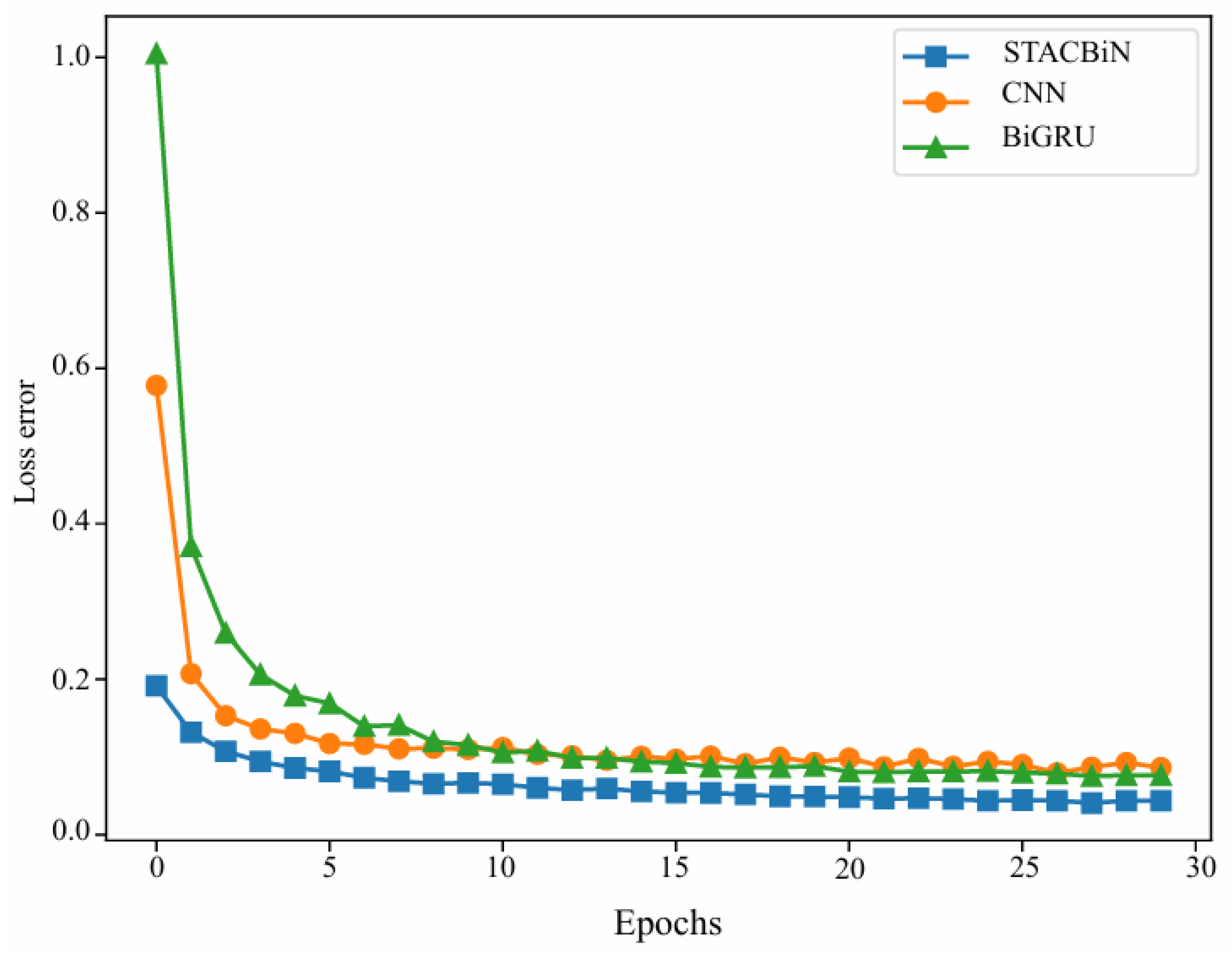
Figure 10 shows the change in the loss error curve of all networks on the training set with the number of training times. It can be seen that the loss errors of all networks decrease continuously with the increase in the number of training times until convergence, indicating that all networks reach the optimal state at this time. Meanwhile, the loss error of the STACBiN integrated network is the lowest, indicating that the predicted values of the network proposed are the closest to the true values.
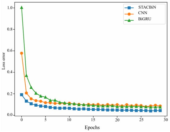
Figure 10.
Loss error curves of the 2DCNN, BiGRU, and STACBiN networks.
4.1. Training Set Analysis
Figure 11 and Table 2 show the forecast results and valuation results of different methods on some training sets, respectively. It can be seen that although the three networks can fit the shear wave velocity well, the fitting effect of the STACBiN integrated network is higher than that of 2DCNN and BiGRU. The R2 between the predicted values and the true values of the STACBiN integrated network reaches 0.9486, which is 0.0168 and 0.0064 higher than that of 2DCNN and BiGRU networks, showing a strong fitting effect.
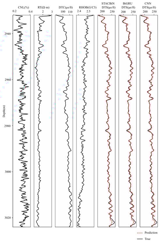
Figure 11.
Prediction results of the STACBiN, BiGRU, and 2DCNN networks in the training set.
Table 2.
Comparison of the prediction results of the 2DCNN, BiGRU, and STACBiN networks in the training set.
4.2. Test Set Analysis
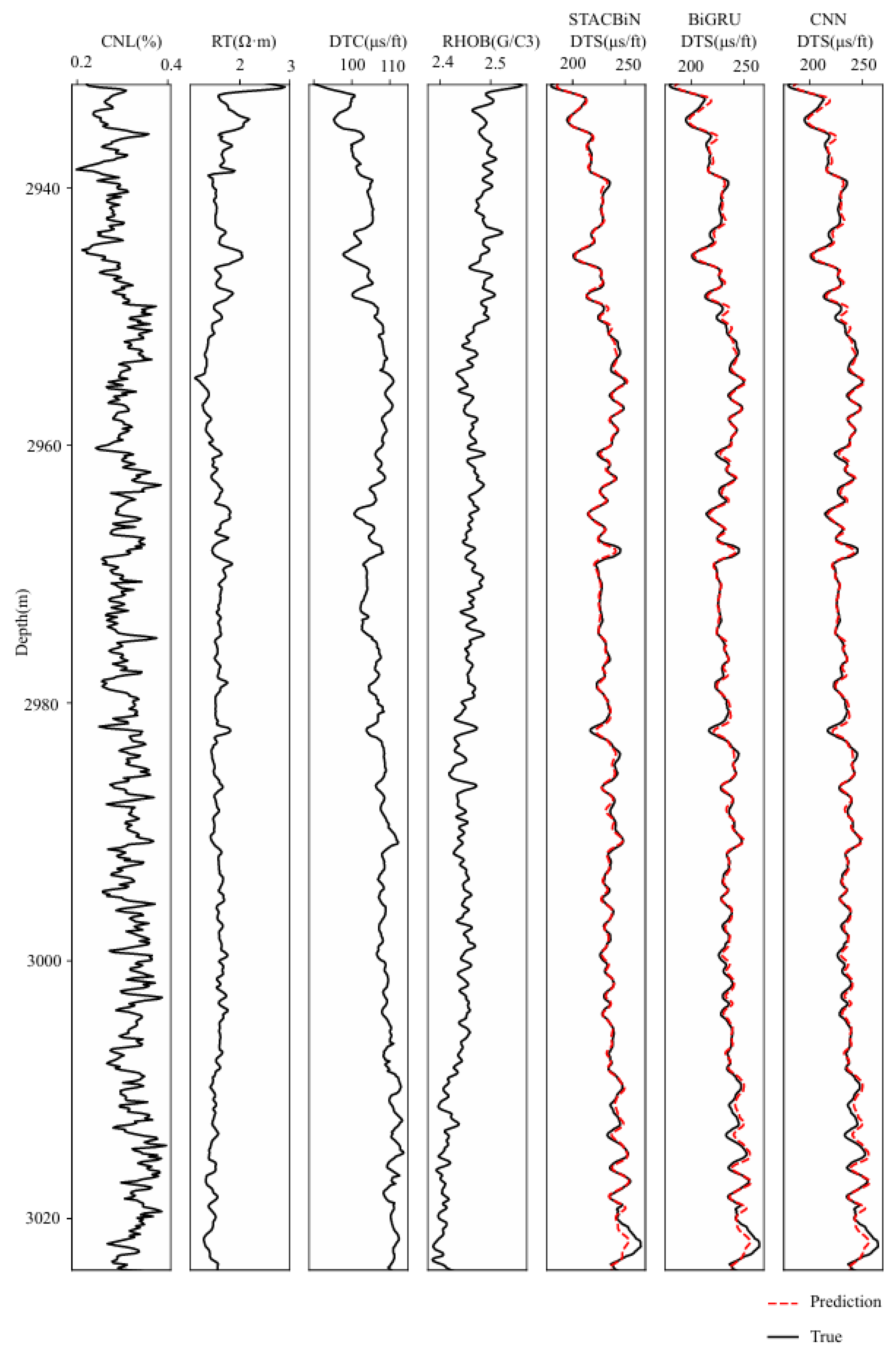
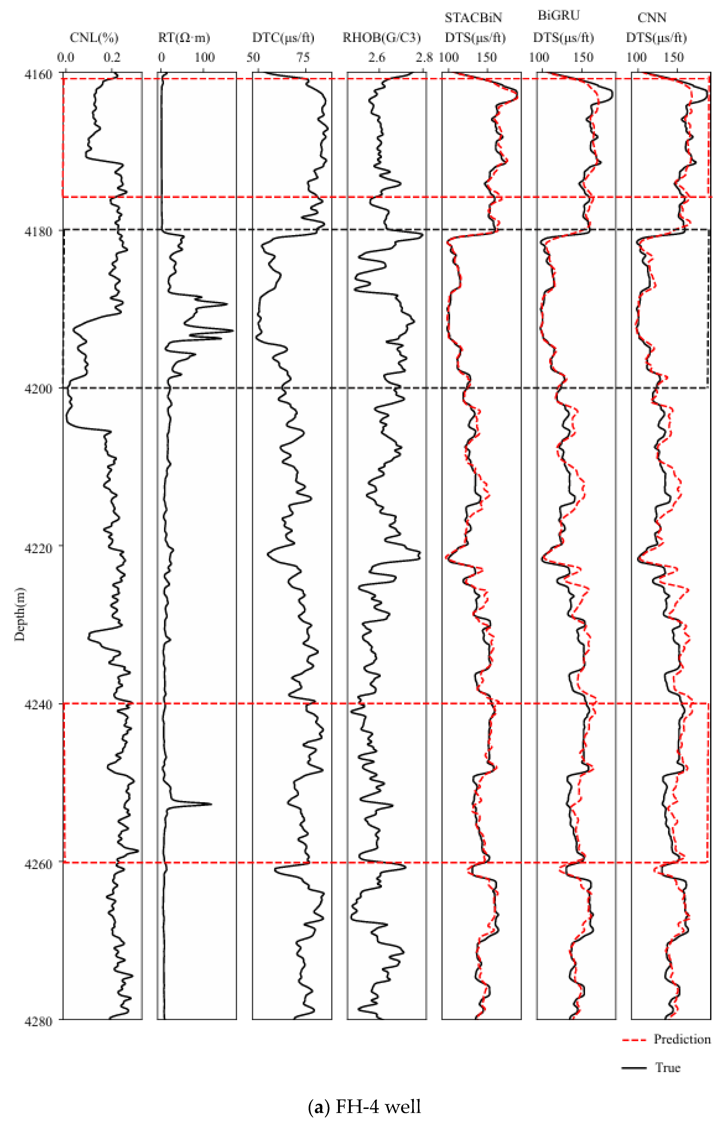
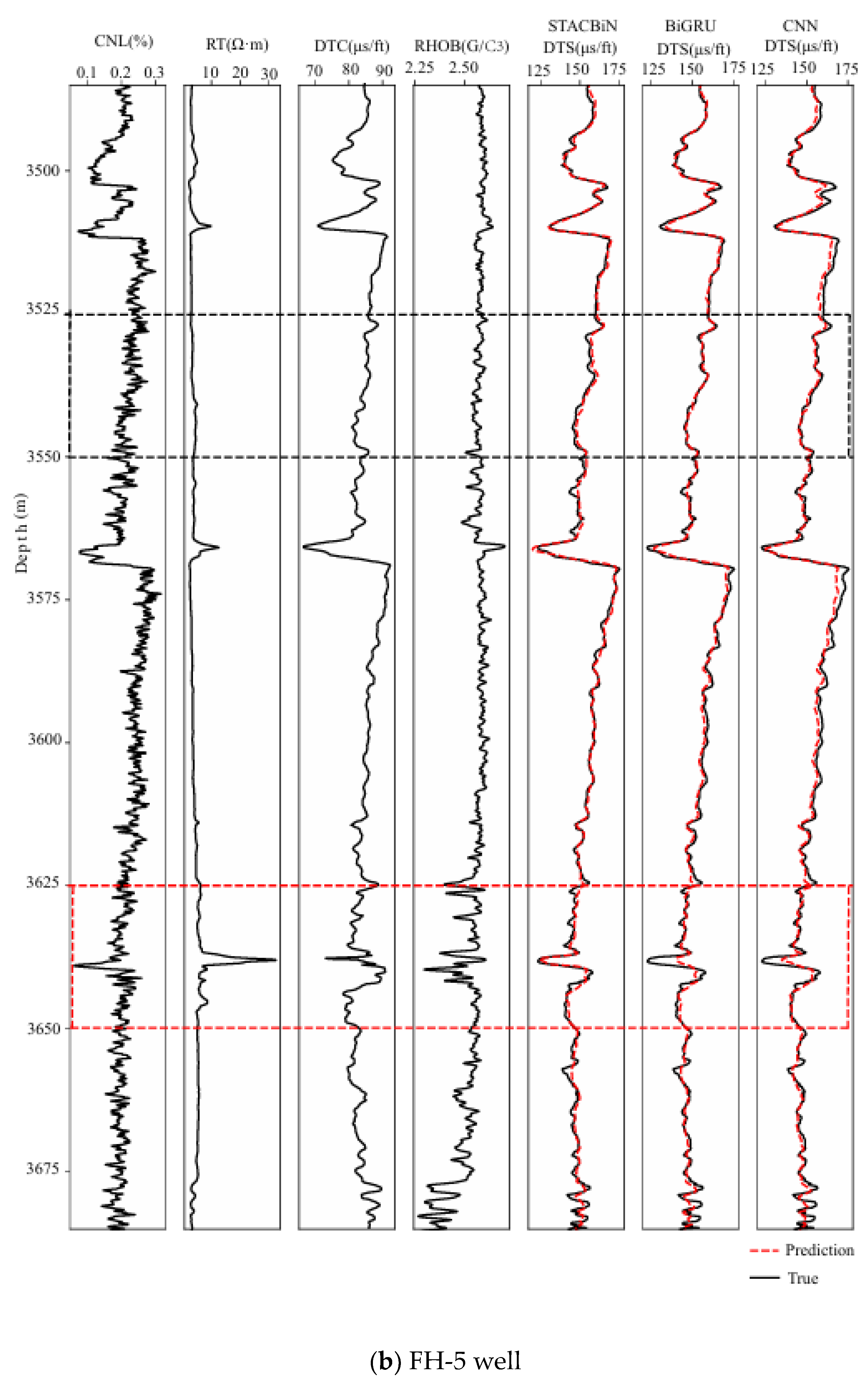
For the sake of proving the effectiveness of the STACBiN integrated network, the three networks trained above are used to predict the shear wave velocity in the FH-4 and FH-5 wells, respectively, and the prediction performance of the three networks is quantitatively evaluated using the evaluation index. In Figure 12, it can be seen that the three methods can establish the mapping relationship between other logging data and shear wave velocity from 4180 m to 4200 m in the FH-4 well and 3525 m to 3550 m in the FH-5 well (black box), and the predicted values are close to the true values. However, the fitting effect of the STACBiN integrated network is better than that of the other two networks from 4160 m to 4175 m and 4240 m to 4260 m in the FH-4 well, and 3625 m to 3650 m in the FH-5 well (red box). The main reason is that the STACBiN integrated network uses 2DCNN and BiGRU networks to obtain the spatial and temporal features of logging data, respectively. At the same time, different spatiotemporal features are assigned different weights so that the network focuses on important spatiotemporal features and ignores irrelevant features, thereby improving the overall performance and prediction accuracy of the network proposed, which makes up for the lack of global perception of 2DCNN and the loss of BiGRU information. Table 3 shows the results of the quantitative evaluation of different methods using MAE and R2. It can be seen that the R2 of the STACBiN integrated network is 0.0261, 0.0121 and 0.0805, 0.0406 higher than that of BiGRU and 2DCNN, respectively, indicating that the network proposed in this paper has high generalization and prediction accuracy.
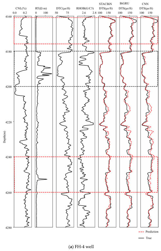
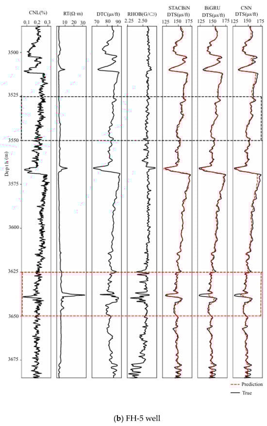
Figure 12.
Prediction results of the STACBiN, BiGRU, and 2DCNN networks in the testing set. ((a) The FH-4 well and (b) FH-5 well).
Table 3.
Comparison of the prediction results of 2DCNN, BiGRU, and STACBiN networks in the testing set.
5. Conclusions
In view of the complex geological conditions of a basin in the South China Sea, considering that the conventional neural network is not sensitive to the spatial and temporal features of logging data, a CNN-BiGRU integrated network based on a spatiotemporal attention mechanism is proposed in this paper, which is applied to the actual data for shear wave velocity prediction, and the effectiveness of the proposed method is verified by two cases. In case 1, the coefficient of attention weight is visualized and analyzed. The weight distribution of spatial attention and temporal attention is consistent with the correlation and autocorrelation of logging data, which verifies the rationality of adding a spatiotemporal attention mechanism. In case 2 on the training set, the R2 of the integrated network is 0.0261 and 0.0121 higher than that of BiGRU, and 0.0805 and 0.0406 higher than that of 2DCNN, respectively, indicating that the neural network based on a spatiotemporal attention mechanism has a stronger fitting effect and generalization than the conventional neural network. The experimental results show that the integrated network based on the spatiotemporal attention mechanism is superior to the conventional neural network in the prediction of shear wave velocity. By adding the spatiotemporal attention mechanism, the network pays more attention to the useful spatiotemporal features, thereby improving the prediction accuracy of the network.
Author Contributions
Conceptualization, Y.L.; Methodology, B.Z.; Software, Y.L.; Formal analysis, Y.L. and B.Z.; Investigation, Y.L.; Writing—original draft, Y.L.; Writing—review & editing, Y.L. and C.G.; Resources, C.G.; Visualization, B.Z.; Supervision, C.G.; Funding acquisition, C.G. All authors have read and agreed to the published version of the manuscript.
Funding
This research is funded by the National Major Science and Technology Project ‘Low Permeability-Tight Gas Reservoir Logging Identification and Comprehensive Evaluation Technology’ (2016ZX05027-002-002).
Data Availability Statement
Data is unavailable due to ethical restrictions.
Conflicts of Interest
The authors declare no conflict of interest.
References
- Castagna, J.P.; Batzle, M.L.; Eastwood, R.L. Relationships between compressional-wave and shear-wave velocities in clastic silicate rocks. Geophysics 1985, 50, 571–581. [Google Scholar] [CrossRef]
- Greenberg, M.L.; Castagna, J.P. Shear-wave velocity estimation in porous rocks: Theoretical formulation, preliminary verification and applications. Geophys. Prospect. 1992, 40, 195–209. [Google Scholar] [CrossRef]
- Kuster, G.T.; Toksöz, M.N. Velocity and attenuation of seismic waves in two-phase media: Part I. Theoretical formulations. Geophysics 1974, 39, 587–606. [Google Scholar] [CrossRef]
- Gurevich, B.; Makarynska, D.; de Paula, O.B.; Pervukhina, M. A simple model for squirt-flow dispersion and attenuation in fluid-saturated granular rocks. Geophysics 2010, 75, N109–N120. [Google Scholar] [CrossRef]
- Xu, S. White R E. A new velocity model for clay-sand mixtures 1. Geophys. Prospect. 1995, 43, 91–118. [Google Scholar] [CrossRef]
- Robert, G.K.; Xu, S.Y. An approximation for the Xu-White velocity model. Geophysics 2002, 67, 1406–1414. [Google Scholar]
- Xu, S.; Payne, M.A. Modeling elastic properties in carbonate rocks. Lead. Edge 2009, 28, 66–74. [Google Scholar] [CrossRef]
- Liu, Y.J.; Li, S.J.; Wang, Y.G.; Xia, Y.H. Reservoir prediction based on shear wave in SuligeGas Field. Oil Geophys. Prospect. 2016, 51. [Google Scholar]
- Zheng, X.Z.; Wang, T.; Liu, Z.; An, T.L. Influence of clay elastic parameters on S-wave velocity estimation based on Xu-White model. Oil Geophys. Prospect. 2017, 52, 990–998. [Google Scholar]
- Li, L.; Ma, J.F.; Zhang, X.X. S-wave velocity prediction in sandstones. Prog. Geophys. 2010, 25, 1065–1074. (In Chinese) [Google Scholar]
- Yang, M.; Li, M.; Li, Y.D.; Lan, F. Prediction of Shear Wave Velocity by Using Optimized Rock Physical Models. J. Oil Gas Technol. 2013, 35, 74–77+3. [Google Scholar]
- Guo, Z.; Li, X. Rock physics model-based prediction of shear wave velocity in the Barnett Shale formation. J. Geophys. Eng. 2015, 12, 527–534. [Google Scholar] [CrossRef]
- Zhang, B.; Liu, C.; Guo, Z.Q.; Liu, X.; Liu, Y. Probabilistic reservoir parameters inversion for anisotropic shale using a statistical rock physics model. Chin. J.Geophys. 2018, 61, 2601–2617. (In Chinese) [Google Scholar]
- Yang, Y.; Yin, X.; Gao, G.; Gui, Z.X.; Zhao, B. Shear-wave velocity estimation for calciferous sandy shale formation. J. Geophys. Eng. 2019, 16, 105–115. [Google Scholar] [CrossRef]
- Chen, Y.; Zhang, X.L.; Li, J.P. Research on application of coal transportation image processing based on deep learning. Autom. Syst. Eng. 2024, 43, 29–35. [Google Scholar]
- Pu, Q.; Yin, S.; Li, Z.M.; Zhao, L.N. Review of U-Net-Based Convolutional Neural Networks for Breast Medical Image Segmentation. J. Front. Comput. Sci. Technol. 2024, 18, 1383–1403. [Google Scholar]
- J, L.; Zhou, Q.D.; Guo, K.; Yang, H.; Lu, B. Energy-saving Design and Research of Hydraulic Control Main Valve of Aerial Work Plat form. Constr. Mach. Equip. 2024, 55, 149–152+261. [Google Scholar]
- LeCun, Y.; Boser, B.; Denker, J.S.; Henderson, D.; Howard, R.E.; Hubbard, W.; Jackel, L.D. Backpropagation applied to handwritten zip code recognition. Neural Comput. 1989, 1, 541–551. [Google Scholar] [CrossRef]
- Schuster, M.; Paliwal, K.K. Bidirectional recurrent neural networks. IEEE Trans. Signal Process. 1997, 45, 2673–2681. [Google Scholar] [CrossRef]
- Creswell, A.; White, T.; Dumoulin, V.; Arulkumaran, K.; Sengupta, B.; Bharath, A.A. Generative adversarial networks: An overview. IEEE Signal Process. Mag. 2018, 35, 53–65. [Google Scholar] [CrossRef]
- Chen, T.; Gao, G.; Li, Y.; Wang, P.; Zhao, B.; Gui, Z.; Zhai, X. Shear-Wave Velocity Prediction Method via a Gate Recurrent Unit Fusion Network Based on the Spatiotemporal Attention Mechanism. Lithosphere 2022, 2022. [Google Scholar] [CrossRef]
- Fang, D.Z.; Ma, W.J.; Yan, X.; Mao, Z.; Gao, Y. Lithology Recognition Research Based on Wavelet Transform and Artificial Intelligence. Well Logging Technol. 2023, 47, 438–446. [Google Scholar]
- Zhou, J.X. Research on inversion algorithm of deep complex in-situ stress field based on depth learning. Chin. J. Rock Mech. Eng. 2024, 43. [Google Scholar]
- Wang, X.G. Application of adaptive BP neural network in shear wave velocity prediction. Lithol. Reserv. 2013, 25, 86–88. [Google Scholar]
- Yang, T.; Cao, D.P.; Du, N.Q.; Cui, R.A.; Nan, F.Z.; Xu, Y.; Liang, C. Prediction of shear wave velocity using receiver functions based on the deep learning method. Chin. J. Geophys. 2022, 65, 214–226. [Google Scholar]
- Ma, Q.Y.; Zhang, X.; Zhang, C.L.; Zhou, H.; Wu, Z.Y. Shear-wave velocity prediction based on one-dimensional convolutional neural net-work. Lithol. Reserv. 2021, 33, 111–120. [Google Scholar]
- Zhou, H.; Wu, Z.Y.; Zhang, X.; Zhang, C.L.; Ma, Q.Y. Shear wave prediction method based on LSTM recurrent neural network. Fault-Block OilGas Field 2021, 28, 829–834. [Google Scholar]
- Wang, J.; Cao, J.; Zhao, S.; Qi, Q.M. S-wave velocity inversion and prediction using a deep hybrid neural network. Sci. China Earth Sci. 2022, 65, 724–741. [Google Scholar] [CrossRef]
- Sun, Y.H.; Liu, Y. Prediction of S-wave velocity based on GRU neural network. Oil Geophys. Prospect. 2020, 55, 484–492, 503. [Google Scholar]
- Teng, J.Q.; Qiu, M.; Yang, M.R.; Shen, H.L.; Qu, S.; Sun, Q.P. Logging curve prediction method based on GRU. Pet. Geol. Recovery Effic. 2023, 30, 93–100. [Google Scholar]
- Chen, T.; Gao, G.; Wang, P.; Zhao, B.; Li, Y.G.; Gui, Z.X. Prediction of shear wave velocity based on a hybrid network of two-dimensional convolutional neural network and gated recurrent unit. Geofluids 2022, 2022. [Google Scholar] [CrossRef]
- Wang, M.; Yang, T. Prediction for Total Porosity of Shale Based on Transfer Deep Neural Network. J. Southwest Pet. Univ. (Sci. Technol. Ed.) 2023, 45, 69–79. [Google Scholar]
- He, K.Y.; Li, Q.C.; Liu, X.Y. Shear wave velocity prediction based on bidirectional long short-term memory networks with attention mechanism. Geophys. Prospect. Pet. 2023, 62, 225–235. [Google Scholar]
- Fu, X.; Wei, Y.; Su, Y.; Hu, H.X. Shear Wave Velocity Prediction Based on the Long Short-Term Memory Network with Attention Mechanism. Appl. Sci. 2024, 14, 2489. [Google Scholar] [CrossRef]
- Qiao, L.; He, N.; Cui, Y.; Zhu, J.C.; Xiao, K. Reservoir Porosity Prediction Based on BiLSTM-AM Optimized by Improved Pelican Optimization Algorithm. Energies 2024, 17, 1479. [Google Scholar] [CrossRef]
- Feng, G.; Liu, W.Q.; Yang, Z.; Yang, W. Shear wave velocity prediction based on 1DCNN-BiLSTM network with attention mechanism. Front. Earth Sci. 2024, 12, 1376344. [Google Scholar] [CrossRef]
- Bengio, Y.; Simard, P.; Frasconi, P. Learning long-term dependencies with gradient descent is difficult. IEEE Trans. Neural Netw. 1994, 5, 157–166. [Google Scholar] [CrossRef]
- Saito, H.; Kato, M. Machine learning technique to find quantum many-body ground states of bosons on a lattice. J. Phys. Soc. Jpn. 2018, 87, 014001. [Google Scholar] [CrossRef]
- Yu, L.; Chen, H.; Dou, Q.; Qin, J.; Heng, P.A. Automated melanoma recognition in dermoscopy images via very deep residual networks. IEEE Trans. Med. Imaging 2016, 36, 994–1004. [Google Scholar] [CrossRef]

Disclaimer/Publisher’s Note: The statements, opinions and data contained in all publications are solely those of the individual author(s) and contributor(s) and not of MDPI and/or the editor(s). MDPI and/or the editor(s) disclaim responsibility for any injury to people or property resulting from any ideas, methods, instructions or products referred to in the content. |
© 2024 by the authors. Licensee MDPI, Basel, Switzerland. This article is an open access article distributed under the terms and conditions of the Creative Commons Attribution (CC BY) license (https://creativecommons.org/licenses/by/4.0/).