A Semi-Global Finite-Time Dynamic Control Strategy of Stochastic Nonlinear Systems

Abstract

In the article, the semi-global finite-time control strategy for stochastic nonlinear systems is studied. Firstly, the general stochastic nonlinear system is considered and the required conditions are provided. An important theorem that helps to construct the controller directly is subsequently obtained by adopting a dynamic gain and homogeneous domination method. The equilibrium of the whole system is semi-global finite-time stable in probability (SGFSP) under the designed controller. Finally, the presented method is successfully applied to a second-order system. Simulation results indicate the effectiveness of the method.

1. Introduction

Numerous practical systems in engineering, for example, chemical reactor systems [1], robot systems [2], and surface ships [3], have the characteristic of nonlinearity. Many excellent methods have recently been reported to tackle control issues in different nonlinear systems [4,5]. Because of work environments or other external factors, many dynamic nonlinear systems inevitably suffer from random noise [6]. For example, ships with random forces coming from the sea [7] and the mechanical system in the randomly changing environment given in [8], and so on. Stochastic nonlinear systems contain plenty of difficulties and challenges for system control and analysis. Since such types of systems have different structures and conditions, it is not possible to use one method to study all systems. In past years, scholars have developed various theories and control strategies to study systems with different structures, including the output feedback control [9], the adaptive control [10], and the intelligent control [11]. However, many control issues remain.

Of the control studies, finite time control has received a lot of attention [12,13,14] since it has more advantages, including faster convergence and better robustness. There currently exist many results for this type of control. Specially, some new sufficient conditions have been provided and finite-time cost controllers derived for the stochastic linear system [15]. For the stochastic nonlinear system, an adaptive finite-time control scheme is proposed in [16]. On the other hand, in practical life, the systems constantly suffer from external disturbances. Because of the existence of the disturbances, achieving the goal of finite time stability is usually difficult. For this reason, semi-global finite-time control design has received a lot of attention. For example, by employing the fuzzy method and command filter approach, the studied systems were guaranteed to be SGFSP [17]. However, based on the existing methods, the designed controllers are somewhat complicated. For example, based on the backstepping method, the obtained controller has a complexity explosion problem. The fuzzy method needs to appropriate the nonlinear functions. Naturally, a question is asked:

Can we present a new semi-global finite control method for a general stochastic nonlinear system to avoid the above problem?

In this article, we plan to consider the above issue. The contributions are twofold.

(i)

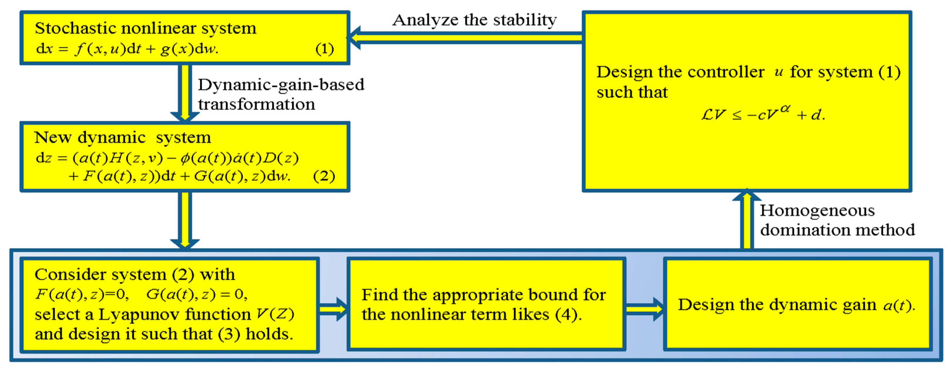
This paper presents a new control strategy. For a general stochastic nonlinear system, we introduce the dynamic-gain-based transformation and obtain a transformed dynamic system. By providing the required conditions and adopting the idea of homogeneous domination, we present a new scheme to construct a dynamic controller, which guarantees that the whole system is SGFSP.

(ii)

The presented strategy is successfully applied to stabilize stochastic nonlinear systems. By imposing the assumptions and verifying all the needed conditions, we flexibly select a new Lyapunov function and provide a detailed design procedure for the studied system. Finally, a dynamic controller is designed.

Notations: The nomenclatures are as follows. $\mathcal{R}$ denotes the set of all real numbers; ${\mathcal{R}}^r$ and ${\mathcal{R}}^n$ are the $r$-dimensional and $n$-dimensional real number spaces, respectively; ${\mathcal{R}}^{n\times r}$ is the set of $n\times r$ real matrix; $\mathrm{Tr}\left\{X\right\}$ is the trace of $X$ when $X$ is square; $E(\cdot )$ is the mathematical expectation; $\mathrm{d}x$ is the differentiation of $x$; $\partial V(z)/\partial z$ represents the partial derivative of the function $V(z)$ for the variable $z$; ${\partial }^{2}V(z)/\partial z_1^2$ represents the second-order partial derivative of the function $V(z)$ for the variable $z_1$; $\dot{a}(t)$ is the time derivative of the function $a(t)$; $\max \left\{b,c\right\}$ represents the maximum number between $b$ and $c$; $\min \left\{b,c\right\}$ represents the minimum value between $b$ and $c$; $\mathcal{L}V$ denotes the differential operator of the function $V.$

2. System, Definition, and Useful Lemmas

In the work, we studied the stochastic nonlinear system [17]

$$\mathrm{d}x=f(x,u)\mathrm{d}t+g(x)\mathrm{d}w,$$

(1)

where $x={(x_1,\dots ,x_n)}^{\top }\in {\mathcal{R}}^n$ is the state vector, $u\in \mathcal{R}$ is the control input, $f\in {\mathcal{R}}^n,g\in {\mathcal{R}}^{n\times r}$ are locally Lipschitz continuous function vector and matrix, respectively. $w\in {\mathcal{R}}^r$ is the r-dimensional standard Wiener process. The goal of the study is to design the controller u such that system (1) is SGFSP.

In stochastic nonlinear system (1), Gauss white noise $\dot{w}$ is considered and is generally viewed as an ideal white noise. The power spectral density of Gaussian white noise follows a uniform distribution, and the amplitude distribution follows a Gaussian distribution. The system states $x_1,\dots ,x_n$ are disturbed.

Remark 1.

The noise used in the proposed model is Gaussian white noise. Its amplitude statistical law follows a Gaussian distribution and the related power spectrum is a constant. The additive noise generally refers to the noise superimposed on a signal, and it always exists regardless of the presence or absence of the signal. It may not necessarily follow a Gaussian distribution, and its power spectral density may not be a constant. The Gaussian white noise has the following benefits: (1) In the process of modeling some stochastic dynamic systems, by assuming that the suffered noise is Gaussian white noise, we can greatly simplify the mathematical modeling problem and provide a more convenient stochastic differential equation model. (2) It has clear characteristics and is easy to handle, so the related analysis will be simplified. (3) It can approximate many noises in the practical world and hence has a wide range of applications in practical engineering.

We need the definition and lemmas as follows.

Definition 

1 ([17]). For system (1), if there is a positive constant $\epsilon$ and a settling time $T(\epsilon ,x_0,w)<\infty$ such that the mathematical expectation of $x(t,w)$ satisfying $E(‖x(t,w)‖)<ϵ,$   $t\ge t_0+T$ then the system equilibrium $x=0$ is SGFSP.

Lemma 1

([13]). There exists an inequality

$$\left|h(w,r)w^{\lambda }{r}^{ϵ}\right|\le c(w,r){\left|w\right|}^{\lambda +ϵ}+|h(w,r){|}^{\frac{\lambda +ϵ}{ϵ}}|r{|}^{\lambda +ϵ}\frac{ϵ}{\lambda +ϵ}{\left(\frac{\lambda }{(\lambda +ϵ)c(w,r)}\right)}^{\frac{\lambda }{ϵ}},$$

where $\lambda ,ϵ$ are positive constants, $h(w,r)>0,c(w,r)>0$ are functions.

Lemma 2

([18]). Let $0\le a_1\le \cdots \le a_n$ and $m_1>0,\cdots ,m_n>0$. If $z\in \mathcal{R},$ there hold

$$m_1|z{|}^{a_1}+m_n|z{|}^{a_n}\le {\displaystyle \sum _{k=1}^n{m}_k}|z{|}^{a_k}\le \left({\displaystyle \sum _{k=1}^n{m}_k}\right)\left(|z{|}^{a_1}+|z{|}^{a_n}\right).$$

Lemma 3

([19]). For $k\ge 1,$ and any real numbers $s, z,$ there holds $|s^k-z^k|\le a|s-z|$$\cdot (|s-z{|}^{k-1}+|z{|}^{k-1}),$ where $a>1$ is a constant.

Lemma 4

([17]). For system (1), If there is a continuous differentiable Lyapunov function $V(x),$ class $K_{\infty }$ functions ${\beta }_1,{\beta }_2$ and constants $c>0, 0<\kappa <1, \rho >0$ such that ${\beta }_1(|x|)<V(x)<{\beta }_2(|x|),$ and $\mathcal{L}V(x)<-V^{\kappa }(x)+\rho ,$ Then, the closed-loop system is semi-global finite-time stable in probability.

3. Dynamic-Gain-Based Homogeneous Domination Method

For the dynamic gain $a(t)$, which satisfies $a(t)\ge 1,\dot{a}(t)\ge 0,$ suppose that there exist coordinate transformations $z_i={\phi }_i(a(t),x_i),i=1,\dots ,n,v={\phi }_{n+1}(a(t),u),$ such that system (1) can be converted to

$$\mathrm{d}z=(a(t)H(z,v)-\varphi (a(t))\dot{a}(t)D(z)+F(a(t),z))\mathrm{d}t+G(a(t),z)\mathrm{d}w,$$

(2)

where $z={(z_1,\dots ,z_n)}^{\top },{\phi }_j(a(t),x_j),j=1,\dots ,n+1$ are continuous functions, $E\in {\mathcal{R}}^n,D\in {\mathcal{R}}^n,$ $F\in {\mathcal{R}}^n$ are continuous function vectors, $G\in {\mathcal{R}}^{n\times r}$ is a matrix, $\varphi (a(t))>0$ is a continuous function.

In this paper, we present a new control strategy using the dynamic gain and homogeneous domination method. The strategy covers the following basic steps: Firstly, it needs to introduce a dynamic-gain-based transformation and transform the original system (1) into a new dynamic system (2). Secondly, consider system (2) when $F(a(t),z)=0,$ $G(a(t),z)=0,$ select a Lyapunov function $V(z)\in {\mathcal{C}}^2$ and design a controller $v(z)$ such that the partial derivative of $V(z)$ along the system satisfies the inequality (3). Thirdly, find the appropriate bounds for nonlinear terms like (4). Fourthly, design the dynamic gain to regulate the bounds of nonlinear terms and compute the differential operator of $V(z)$ such that it satisfies a form that is convenient for stability analysis. Finally, construct the controller of the original system (1) using the controller $v(z)$ and the dynamic-gain-based transformation and analyze the system stability. The diagram of the control strategy is provided in Figure 1.

Next, we summarize the strategy using the following theorem.

Theorem 1.

For system (2), suppose there is a continuously differentiable positive definite Lyapunov function$V(z)\in {\mathcal{C}}^2$and a smooth controller$v(z)=\chi (z)$ such that

$$\frac{\partial V(z)}{\partial z}(a(t)H(z,\chi (z))-\varphi (a(t))\dot{a}(t)D(z))\le -c_{1}a(t)({\displaystyle \sum _{i=1}^2{U}_i}(z))-c_2\varphi (a(t))\dot{a}(t)({\displaystyle \sum _{i=3}^4{U}_i}(z)),$$

(3)

and

$$\left|\frac{\partial V(z)}{\partial z}F+\frac{1}{2}Tr\left\{G\frac{{\partial }^{2}V(z)}{\partial z^2}{G}^{\top }\right\}\right|\le c_3{a}^{1-s}(t){\displaystyle \sum _{i=1}^2{U}_i}(z)+{\delta }_0,$$

(4)

where$c_j>0,1\le j\le 3$ are constants, $U_i(z),1\le i\le 4$ are positive definite functions, $V(z)$ satisfies $c_4{V}^{\alpha }(z)\le {\displaystyle \sum _{i=1}^2{U}_i}(z)+d_0$ for some positive constants $c_4$ and $d_0$. $U_j(z),1\le j\le 2$ satisfy the inequality $U_j(z)\le U_3(z){\psi }_j(z),$ where ${\psi }_j(z)\ge 0$ is a continuous function. $a(t)$ satisfies $\dot{a}(t)\ge 0$. Afterward, we can construct a dynamic-gain-based controller that is specified as $u=T_2^{-1}(a(t),\chi (T_1(a(t),x))),$  $\dot{a}(t)={\displaystyle \sum _{j=1}^2{\psi }_j}(z)\max \left\{-\frac{c_1}{2c_2\varphi (a(t))}a(t)+\frac{c_3}{c_2\varphi (a(t))}{a}^{1-s}(t),0\right\},$  $a(0)\ge 1,$ which guarantees system (1) is SGFSP.

Proof of Theorem 1.

For system (2), we choose the Lyapunov function $V(z),$ then the differential operator of $V(z)$ satisfies

$$\begin{array}{l}\mathcal{L}V=\frac{\partial V(z)}{\partial z}(a(t)H(z,\chi (z))-\varphi (a(t))\dot{a}(t)D(z))+\left|\frac{\partial V(z)}{\partial z}F+\frac{1}{2}\mathrm{Tr}\left\{G^T\frac{{\partial }^{2}V(z)}{\partial z^2}G\right\}\right|\\ \hspace{1em}\hspace{0.33em}\hspace{0.17em} \le -c_{1}a(t)({\displaystyle \sum _{i=1}^2{U}_i}(z))-c_2\varphi (a(t))\dot{a}(t)({\displaystyle \sum _{i=3}^4{U}_i}(z))n+c_3{a}^{1-s}(t)({\displaystyle \sum _{i=1}^2{U}_i}(z))+{\delta }_0.\end{array}$$

Using (4) and the relationship $U_j(z)=U_3(z){\psi }_j(z),1\le j\le 2,$ we get

$$\begin{array}{l}\mathcal{L}V=\frac{\partial V(z)}{\partial z}(a(t)H(z,\chi (z))-\varphi (a(t))\dot{a}(t)D(z))\\ \hspace{1em} \le -c_{1}a(t)({\displaystyle \sum _{i=1}^2{U}_i}(z))-c_2\varphi (a(t))\dot{a}(t)U_3(z)+c_3{a}^{1-s}(t)({\displaystyle \sum _{i=1}^2{U}_i}(z))+{\delta }_0\\ \hspace{1em}\hspace{0.33em}\hspace{0.33em}\le -\frac{c_1}{2}a(t)({\displaystyle \sum _{i=1}^2{U}_i}(z))-U_3(z)(c_2\varphi (a(t))\dot{a}(t)+\frac{c_1}{2}a(t){\displaystyle \sum _{j=1}^2{\psi }_j}(z)-c_3{a}^{1-s}(t){\displaystyle \sum _{j=1}^2{\psi }_j}(z))+{\delta }_0.\end{array}$$

Choosing the dynamic gain $\dot{a}(t)={\displaystyle \sum _{j=1}^2{\psi }_j}(z)\max \left\{\frac{c_1}{2c_2\varphi (a(t))}a(t)+\frac{c_3}{c_2\varphi (a(t))}{a}^{1-s}(t),0\right\},$ one has

$$\mathcal{L}V\le -\frac{c_1}{2}a(t)({\displaystyle \sum _{i=1}^2{U}_i}(z))+{\delta }_0\le -\frac{c_1}{2}({\displaystyle \sum _{i=1}^2{U}_i}(z))+{\delta }_0\le \frac{c_1}{2}(-V^{\alpha }(z)+d_0)+{\delta }_0\le -c{V}^{\alpha }(z)+d,$$

where $c=\frac{c_1}{2},d=\frac{c_1}{2}{d}_0+{\delta }_0.$ Using Theorem 1 in [17], we see the equilibrium $z=0$ of system (2) is SGFTS, that is, there is a ${ϵ}_1>0$ and a settling time $T_s({ϵ}_1,z_0,w)<\infty$ such that mathematical expectation of $z(t,w)$ satisfying $E(‖z(t,w)‖)<{ϵ}_1,t\ge T_s$. In view of the constructed dynamic gain $a(t)$ assuming the existence of finite time $T_0$ to make $a(T_0)\ge {\left(c_1/(2c_3)\right)}^{1/s},$ one has $\dot{a}(t)<0,\forall t\in [T_0,+\infty )$. Thus, the boundedness of $a(t)$ has been proven. Otherwise, one gets $a(t)\le {\left(c_1/(2c_3)\right)}^{1/s},\forall t\in [0,T_0)$. Using the above proof, it can be inferred that $a(t)<{ϵ}_2,\forall t\in [0,+\infty )$ with ${ϵ}_2$ being a constant. For a continuous function $z_i={\phi }_i(a(t),x_i),$ its inverse function $x_i={\phi }_i^{-1}(a(t),z_i)$ is also a continuous function. Due to the boundedness of continuous functions on closed intervals, when the conditions $E(z_i)\in [0,{ϵ}_1],a(t)\in [0,{ϵ}_2]$ are met, there is a constant $\overline{ϵ}$ that makes $E(‖x_i(t,w)‖)=E(‖{\phi }_i^{-1}(a(t),z_i(t))‖)<\overline{ϵ}$. Therefore, there exists the constant $\sigma \ge \overline{ϵ}$ together with a settling time $T_s(\sigma ,x_0,w)<\infty$ such that mathematical expectations of $x_i(t,w)$ satisfy $E(‖x_i(t,w)‖)<\sigma ,1\le i\le n,t\ge T_s,$ which shows that system (1) is SGFSP. ◻

4. Control of Second-Order Stochastic Nonlinear System

As an application, we consider the following system

$$\left\{\begin{array}{l}\mathrm{d}{x}_1=(x_2^p+f_1(x_1))\mathrm{d}t+g_1(x_1)\mathrm{d}w,\hfill \\ \mathrm{d}{x}_2=(u^p+f_2(x_1,x_2))\mathrm{d}t+g_2(x_1,x_2)\mathrm{d}w,\hfill \end{array}\right.$$

(5)

where $x_1,x_2$ are the states, $u$ is the control input, and $p\ge 1$ is an odd integer. The other symbols are defined as in (1).

We next provide some conditions.

Assumption 1.

For  $1\le i\le 2,$ functions $f_i$ and $g_i$ satisfy

$$|f_i(\cdot )|\le C{\displaystyle \sum }_{j=1}^i{\left|x_j\right|}^p+\delta ,\hspace{0.33em}\hspace{0.33em}\hspace{0.33em} |g_i(\cdot )|\le C{\displaystyle \sum }_{j=1}^i{\left|x_j\right|}^{\frac{p+1}{2}}+\delta ,$$

where $C,\delta$ are positive constants.

Introduce the transformations $z_1=x_1/a^{{\epsilon }_1}(t),z_2=x_2/a^{{\epsilon }_2}(t),v=u/a^{{\epsilon }_3}(t),$ where $s>0$ is a constant ($s=1$ for $p=1;$ $s=1/p^{n-1}-(p-1){\epsilon }_1/p^{n-1}$ for $p>1$), ${\epsilon }_1\le p^{n-1}/(p-1+p^{n-1}),$ ${\epsilon }_2=({\epsilon }_1+1)/p,$ ${\epsilon }_3=({\epsilon }_2+1)/p$ are constants. Then, system (5) is transformed into

$$\mathrm{d}z=(a(t)H(z,v)-\varphi (a(t))\dot{a}(t)D(z)+F(a(t),z))\mathrm{d}t+G(a(t),z)\mathrm{d}w,$$

with $H(z,v)={(z_2^p, v^p)}^{\top },\varphi (a(t))=1/a(t), D(z)={({\epsilon }_1{z}_1,{\epsilon }_2{z}_2)}^{\top }, F(a(t),z)={(f_1/a^{{\epsilon }_1}(t),f_2/a^{{\epsilon }_2}(t))}^{\top }$ and $G(a(t),z)={(g_1/a^{{\epsilon }_1}(t),g_2/a^{{\epsilon }_2}(t))}^{\top }.$ Next, we have the following control results.

Theorem 2.

For system (2) under Assumption 1, there is the following dynamic-gain-based controller

$$\left\{\begin{array}{l}u=-a^{{\epsilon }_3}(t){\beta }_2{\chi }_2(z),\hfill \\ \dot{a}(t)=\frac{c_1}{2c_2}({\displaystyle \sum _{j=1}^2{\psi }_j}(z))\max \{\frac{2c_3}{c_1}{a}^{2-s}(t)-a^2(t),0\},\hfill \end{array}\right.$$

where ${\chi }_1(z)=z_1,{\chi }_2(z)=z_2+{\beta }_1{z}_1. {\beta }_1,{\beta }_2$ are positive constants to be defined. The designed controller ensures that the equilibrium $x_1=x_2=0$ of system (5) is SGFSP.

Proof. 

We choose the Lyapunov function $V=\rho V_1+V_2,V_i=1/4{\chi }_i^4(z)+1/(p+3){\chi }_i^{p+3}(z),$   $i=1,2,$ where $\rho$ is a positive constant. It can be verified that ${\gamma }_1(\left|z\right|)\le V(z)\le {\gamma }_2(\left|z\right|),$where ${\gamma }_j, j=1,2$ are class ${\mathcal{K}}_{\infty }$ functions. Considering the auxiliary system

$$\mathrm{d}z=(a(t)H(z,v)-\varphi (a(t))\dot{a}(t)D(z))\mathrm{d}t,$$

(6)

i.e., the following system

$$\left\{\begin{array}{l}\mathrm{d}{z}_1=(a(t)z_2^p-\varphi (a(t))\dot{a}(t){\epsilon }_1{z}_1)\mathrm{d}t,\hfill \\ \mathrm{d}{z}_2=(a(t)v^p-\varphi (a(t))\dot{a}(t){\epsilon }_2{z}_2)\mathrm{d}t.\hfill \end{array}\right.$$

(7)

In the following, we provide the detailed control design steps for system (7) and show that the inequality (3) holds.

• Step 1. By the definition ${\chi }_1(z)=z_1,$ choose the function $V_1=1/4{\chi }_1^4(z)+1/(p+3){\chi }_1^{p+3}(z),$ then the differential operator of $V_1(z)$ satisfies

  $$\begin{array}{l}\mathcal{L}{V}_1=\frac{\partial V_1(z)}{\partial z_1}(a(t)z_2^p-\varphi (a(t))\dot{a}(t){\epsilon }_1{z}_1)\\ \hspace{1em}\hspace{0.33em}\hspace{0.33em}=({\chi }_1^3(z)+{\chi }_1^{p+2}(z))a(t)(z_2^p-{\pi }^p(z))\\ \hspace{1em}\hspace{1em}\hspace{0.33em}+({\chi }_1^3(z)+{\chi }_1^{p+2}(z))a(t){\pi }^p(z)-\varphi (a(t))\dot{a}(t){\epsilon }_1({\chi }_1^4(z)+{\chi }_1^{p+3}(z)).\end{array}$$

  (8)

  Choosing the virtual controller $\pi (z)=-{\beta }_1{\chi }_1,{\beta }_1\ge b_0^{1/p}$ with $b_0$ being a positive constant and substituting it into (8), we get

  $$\begin{array}{l}\mathcal{L}{V}_1\le -b_{0}a(t)({\chi }_1^{p+3}(z)+{\chi }_1^{2p+2}(z))-\varphi (a(t))\dot{a}(t){\epsilon }_1({\chi }_1^4(z)+{\chi }_1^{p+3}(z))\\ \hspace{1em}\hspace{0.33em}\hspace{0.33em}+({\chi }_1^3(z)+{\chi }_1^{p+2}(z))a(t)(z_2^p-{\pi }^p(z)).\end{array}$$
• Step 2. Noting ${\chi }_2(z)=z_2+{\beta }_1{z}_1,V=\rho V_1+(1/4{\chi }_1^4(z)+1/(p+3){\chi }_2^{p+3}(z)),$ it is deduced that

  $$\begin{array}{l}\mathcal{L}V\le \rho \mathcal{L}{V}_1+({\chi }_2^3(z)+{\chi }_2^{p+2}(z))a(t)v^p+{\beta }_1({\chi }_2^3(z)+{\chi }_2^{p+2}(z))(a(t)z_2^p-\varphi (a(t))\dot{a}(t){\epsilon }_1{z}_1)\\ \hspace{1em}\hspace{1em}\hspace{0.17em}-\varphi (a(t))\dot{a}(t){\epsilon }_2({\chi }_2^3(z)+{\chi }_2^{p+2}(z))z_2\\ \hspace{1em}\hspace{0.33em}\hspace{0.33em}\le ({\chi }_2^3(z)+{\chi }_2^{p+2}(z))a(t)v^p+{\beta }_1({\chi }_2^3(z)+{\chi }_2^{p+2}(z))(a(t)z_2^p-\varphi (a(t))\dot{a}(t){\epsilon }_1{z}_1)\\ \hspace{1em}\hspace{1em}\hspace{0.33em}-\varphi (a(t))\dot{a}(t){\epsilon }_2({\chi }_2^3(z)+{\chi }_2^{p+2}(z))z_2-b_0\rho a(t)({\chi }_1^{p+3}(z)+{\chi }_1^{2p+2}(z))\\ \hspace{1em}\hspace{1em}\hspace{0.33em}-\varphi (a(t))\dot{a}(t){\epsilon }_1\rho ({\chi }_1^4(z)+{\chi }_1^{p+3}(z))+\rho ({\chi }_1^3(z)+{\chi }_1^{p+2}(z))a(t)(z_2^p-{\pi }^p(z)).\end{array}$$

  (9)

  Using Lemma 3, we have $|z_2^p-{\pi }^p|\le p|{\chi }_2|(|{\chi }_2{|}^{p-1}+|{\beta }_1{\chi }_1{|}^{p-1})\le p|{\chi }_2{|}^p+p{\beta }_1^{p-1}|{\chi }_2||{\chi }_1{|}^{p-1},$ from which Lemma 1 indicates

  $$\begin{array}{l}\rho ({\chi }_1^3(z)+{\chi }_1^{p+2}(z))a(t)(z_2^p-{\pi }^p(z))\\ \le a(t)\rho b_0/2({\chi }_1^{p+3}(z)+{\chi }_1^{2p+2}(z))+a(t)\rho (A_1+A_2)({\chi }_2^{p+3}(z)+{\chi }_2^{2p+2}(z)),\end{array}$$

  (10)

  where $A_1=\frac{p}{p+3}{(\frac{12}{b_0(p+3)})}^{\frac{p+3}{p}}{p}^{\frac{p+3}{p}}+\frac{p}{2p+2}{(\frac{4(p+2)}{b_0(2p+2)})}^{\frac{p+2}{p}}{p}^{\frac{2p+2}{p}},$ $A_2=\frac{1}{p+3}{(\frac{4(p+2)}{b_0(p+3)})}^{p+2}$ $\cdot {(p{\beta }_1^{p-1})}^{p+3}+\frac{1}{2p+2}{(\frac{4(2p+1)}{b_0(2p+2)})}^{2p+1}{(p{\beta }_1^{p-1})}^{2p+2}.$ Given Lemma 1 and $z_2={\chi }_2(z)$ $-{\beta }_1{\chi }_1(z),$ there holds

  $$\begin{array}{l}-\varphi (a(t))\dot{a}(t){\epsilon }_2({\chi }_2^3(z)+{\chi }_2^{p+2}(z))z_2\\ \le -\varphi (a(t))\dot{a}(t){\epsilon }_2(1-{\gamma }_1)({\chi }_2^4(z)+{\chi }_2^{p+3}(z))+\varphi (a(t))\dot{a}(t)B_1({\chi }_1^4(z)+{\chi }_1^{p+3}(z)),\end{array}$$

  (11)

  where $0<{\gamma }_1<1$ and $B_1=\frac{1}{4}{(\frac{3}{4{\gamma }_1})}^3{\beta }_1^4{\epsilon }_2+\frac{1}{p+3}{(\frac{p+2}{{\gamma }_1(p+3)})}^{p+2}{\beta }_1^{p+3}{\epsilon }_2$ are constants. Considering $z_1={\chi }_1(z),z_2={\chi }_2(z)-{\beta }_1{\chi }_1(z)$ and applying $|y_1+y_2{|}^k\le 2^{k-1}(|y_1{|}^k+|y_2{|}^k),$ it yields that $|z_2{|}^p=|{\chi }_2(z)-{\beta }_1{\chi }_1(z){|}^p\le 2^{p-1}(|{\chi }_2(z){|}^p+|{\beta }_1{\chi }_1(z){|}^p)\le 2^{p-1}|{\chi }_2(z){|}^p+2^{p-1}{\beta }_1^p|{\chi }_1(z){|}^p.$ Thus, it follows from Lemma 1 that

  $$\begin{array}{l}{\beta }_1({\chi }_2^3(z)+{\chi }_2^{p+2}(z))(a(t)z_2^p-\varphi (a(t))\dot{a}(t){\epsilon }_1{z}_1)\\ \le a(t)\rho b_0/4({\chi }_1^{p+3}(z)+{\chi }_1^{2p+2}(z))+a(t)\rho (A_3+2^{p-1}{\beta }_1)({\chi }_2^{p+3}(z)+{\chi }_2^{2p+2}(z)) \\ \hspace{0.33em}\hspace{0.17em}\hspace{0.17em}+\varphi (a(t))\dot{a}(t){\epsilon }_2{\gamma }_2({\chi }_2^4(z)+{\chi }_2^{p+3}(z))+\varphi (a(t))\dot{a}(t)B_2({\chi }_1^4(z)+{\chi }_1^{p+3}(z)),\end{array}$$

  (12)

  where ${\gamma }_2$ is a constant and satisfies $0<{\gamma }_2<1-{\gamma }_1,A_3=\frac{3}{p+3}{(\frac{4p}{\rho b_0(p+3)})}^{\frac{p}{3}}{(2^{p-1}{\beta }_1^{p+1})}^{\frac{p+3}{3}}$ $+\frac{p+3}{2p+2}{(\frac{2(p-1)}{\rho b_3(p+1)})}^{\frac{p-1}{p+3}}{(2^{p-1}{\beta }_1^{p+1})}^{\frac{2p+2}{p+3}},B_2=\frac{1}{4}{(\frac{3}{4{\epsilon }_2{\gamma }_2})}^3{({\beta }_1{\epsilon }_1)}^4+\frac{1}{p+3}{(\frac{p+2}{{\gamma }_2{\epsilon }_2(p+3)})}^{p+2}{({\beta }_1{\epsilon }_1)}^{p+3}.$ Putting (10)–(12) into (9) gives

  $$\begin{array}{l}\mathcal{L}V\le -1/4b_0\rho a(t)({\chi }_1^{p+3}(z)+{\chi }_1^{2p+2}(z))-\varphi (a(t))\dot{a}(t)(\rho {\epsilon }_1-B_1-B_2)({\chi }_1^4(z)+{\chi }_1^{p+3}(z))\\ \hspace{1em}\hspace{1em}\hspace{0.33em}-\varphi (a(t))\dot{a}(t){\epsilon }_2(1-{\gamma }_1-{\gamma }_2)({\chi }_2^4(z)+{\chi }_2^{p+3}(z))+({\chi }_2^3(z)+{\chi }_2^{p+2}(z))a(t)v^p\\ \hspace{1em}\hspace{1em}\hspace{0.33em}+a(t)(\rho {\displaystyle \sum _{j=1}^3{A}_j}+2^{p-1}{\beta }_1)({\chi }_2^{p+3}(z)+{\chi }_2^{2p+2}(z)).\end{array}$$

  If we choose $\rho$ satisfying $\rho {\epsilon }_1-B_1-B_2>0,$ define $c_1=1/4b_0\rho ,c_2=\min \{\rho {\epsilon }_1-B_1-B_2,{\epsilon }_2(1-{\gamma }_1-{\gamma }_2)\},$ and design $v=-(\rho {\displaystyle \sum _{j=1}^3{A}_j}+2^{p-1}{\beta }_1+1/4b_0){\chi }_2=:-{\beta }_2{\chi }_2(z),$ then it follows that

  $$\mathcal{L}V\le -c_{1}a(t){\displaystyle \sum _{i=1}^2(}{\chi }_i^{p+3}(z)+{\chi }_i^{2p+2}(z))-c_2\varphi (a(t))\dot{a}(t){\displaystyle \sum _{i=1}^2(}{\chi }_i^4(z)+{\chi }_i^{p+3}(z)).$$

  (13)

  Now, considering (6) and (13), it yields $\frac{\partial V(z)}{\partial z}(a(t)H(z,\chi (z))-\varphi (a(t))\dot{a}(t)D(z))\le -c_{1}a(t)$ $\cdot {\displaystyle \sum _{i=1}^2{U}_i}(z)-c_2\varphi (a(t))\dot{a}(t){\displaystyle \sum _{i=3}^4{U}_i}(z),U_1(z)={\displaystyle \sum _{j=1}^2{\chi }_j^{p+3}}(z),U_2(z)={\displaystyle \sum _{j=1}^2{\chi }_j^{2p+2}}(z),U_3(z)={\displaystyle \sum _{j=1}^2{\chi }_j^{p+3}}(z),$ $U_4(z)={\displaystyle \sum _{j=1}^2{\chi }_j^4}(z).$ Besides, by the definition of $V=\rho (\frac{1}{4}{\chi }_1^4(z)+\frac{1}{p+3}{\chi }_1^{p+3}(z))+(\frac{1}{4}{\chi }_2^4(z)$ $+\frac{1}{p+3}{\chi }_2^{p+3}(z))$ and ${\chi }_2(z)=z_2+{\beta }_1{\chi }_1(z),$ it is easy to deduce that

  $$\frac{\partial V(z)}{\partial z_1}=\rho ({\chi }_1^3(z)+{\chi }_1^{p+2}(z))+{\beta }_1({\chi }_2^3(z)+{\chi }_2^{p+2}(z)),\hspace{1em}\hspace{0.33em}\hspace{0.33em}\hspace{0.33em}\frac{\partial V(z)}{\partial z_2}={\chi }_2^3(z)+{\chi }_2^{p+2}(z).$$

  (14)

  In view of $z_1=x_1/a^{{\epsilon }_1}(t),z_2=x_2/a^{{\epsilon }_2}(t),{\chi }_1(z)=z_1,{\chi }_2(z)=z_2+{\beta }_1{z}_1$ and based on Assumption 1, one can find a constant $\overline{c}$ satisfying

  $$|f_1{a}^{-{\epsilon }_1}(t)|\le a^{1-s}(t)\overline{c}|{\chi }_1{|}^p+\delta ,\hspace{1em}\hspace{0.33em}\hspace{0.33em}\hspace{0.33em}|f_2{a}^{-{\epsilon }_2}(t)|\le a^{1-s}(t)\overline{c}(|{\chi }_1{|}^p+|{\chi }_2{|}^p)+\delta .$$

  (15)

  Noting (14), (15), and Lemma 1, there are constants $l_{21},l_{22},{\overline{\delta }}_0$ such that

  $$\begin{array}{l}\frac{\partial V(z)}{\partial z}F\le \hspace{0.17em}\hspace{0.17em}|\frac{\partial V(z)}{\partial z_1}{f}_1{a}^{-{\epsilon }_1}(t)|+|\frac{\partial V(z)}{\partial z_2}{f}_2{a}^{-{\epsilon }_2}(t)|\\ \hspace{1em}\hspace{1em}\hspace{0.33em}\le a^{1-s}(t)l_{21}({\chi }_1^{p+3}(z)+{\chi }_1^{2p+2}(z))+a^{1-s}(t)l_{22}({\chi }_2^4(z)+{\chi }_2^{p+3}(z))+{\overline{\delta }}_0.\end{array}$$

  Defining ${\overline{c}}_3=\max \{l_{21},l_{22}\},$ it shows that $\frac{\partial V(z)}{\partial z}F\le {\overline{c}}_3{a}^{1-s}(t){\displaystyle \sum _{i=1}^2{U}_i}(z)+{\overline{\delta }}_0.$ It is easy to get

  $$\begin{array}{l}\frac{{\partial }^{2}V(z)}{\partial z_1^2}=\rho (3{\chi }_1^2(z)+(p+2){\chi }_1^{p+1}(z))+{\beta }_1^2(3{\chi }_2^2(z)+(p+2){\chi }_2^{p+1}(z)),\\ \frac{{\partial }^{2}V(z)}{\partial z_1\partial z_2}={\beta }_1(3{\chi }_2^2(z)+(p+2){\chi }_2^{p+1}(z)),\frac{{\partial }^{2}V(z)}{\partial z_2^2}=3{\chi }_2^2(z)+(p+2){\chi }_2^{p+1}(z).\end{array}$$

  (16)

  In addition, there is a constant $\widehat{c}>0$ such that

  $$|g_1{a}^{-{\epsilon }_1}(t)|\le a^{\frac{1-s}{2}}(t)\widehat{c}|{\chi }_1{|}^{\frac{p+1}{2}}+\delta ,\hspace{1em}\hspace{0.33em}\hspace{0.33em}\hspace{0.33em}|g_2{a}^{-{\epsilon }_2}(t)|\le a^{\frac{1-s}{2}}(t)\widehat{c}(|{\chi }_1{|}^{\frac{p+1}{2}}+|{\chi }_2{|}^{\frac{p+1}{2}})+\delta .$$

  (17)

  By Lemma 1, (16) and (17), there are constants ${\widehat{c}}_3$ and ${\widehat{\delta }}_0$ such that

  $$\frac{1}{2}\mathrm{Tr}\left\{G\frac{{\partial }^{2}V(z)}{\partial z^2}{G}^{\top }\right\}\le \frac{1}{2}{\displaystyle \sum _{i,j=1}^2|}\frac{{\partial }^{2}V(z)}{\partial z_i\partial z_j}||g_i{a}^{-{\epsilon }_i}(t)||g_j{a}^{-{\epsilon }_j}(t)|\le {\widehat{c}}_3{a}^{1-s}(t){\displaystyle \sum _{i=1}^2{U}_i}(z)+{\widehat{\delta }}_0.$$

  Then, we can deduce that $\frac{1}{2}\mathrm{Tr}\left\{G\frac{{\partial }^{2}V(z)}{\partial z^2}{G}^{\top }\right\}\le {\widehat{c}}_3{a}^{1-s}(t){\displaystyle \sum _{i=1}^2{U}_i}(z)+{\widehat{\delta }}_0,$. Please refer to the appendix for detailed proofs of the above inequalities. Now, defining $c_3={\overline{c}}_3+{\widehat{c}}_3,$ and ${\delta }_0={\overline{\delta }}_0+{\widehat{\delta }}_0,$ it yields that (4) holds. In addition, it is not difficult to obtain $c_4{V}^{\alpha }(z)\le {\displaystyle \sum _{i=1}^2{U}_i}(z)+d_0,$ where $c_4=\min \{{(1/(p+3))}^{-\alpha },{(1/4)}^{-\alpha }\},d_0=4(1-\alpha )+4(1-4\alpha /(2p+2)).$ Also, there holds $U_j(z)\le U_3(z){\psi }_j(z),1\le j\le 2,$ where ${\psi }_1(z)=1,{\psi }_2(z)={\displaystyle \sum _{j=1}^2{\chi }_j^{p-1}}(z).$ Hence, all conditions of Theorem 1 are satisfied. Then, for system (5), using Theorem 1, we can construct the dynamic-gain-based controller

  $$\left\{\begin{array}{l}u=-a^{{\epsilon }_3}(t){\beta }_2{\chi }_2(z),\hfill \\ \dot{a}(t)=\frac{c_1}{2c_2}({\displaystyle \sum _{j=1}^2{\psi }_j}(z))\max \{\frac{2c_3}{c_1}{a}^{2-s}(t)-a^2(t),0\},\hfill \end{array}\right.$$

  such that the equilibrium $x_1=x_2=0$ of system (5) is SGFSP.◻

Remark 2.

In fact, the presented approach can be applied to more general systems. For example, consider the following stochastic nonlinear system

$$\left\{\begin{array}{l}\mathrm{d}{x}_i=(x_{i+1}+f_i(x_1,\dots ,x_n))\mathrm{d}t+g_i(x_1,\dots ,x_n)\mathrm{d}w, i=1,2,\dots n-1,\hfill \\ \mathrm{d}{x}_n=(u+f_n(x_1,\dots ,x_n))\mathrm{d}t+g_n(x_1,\dots ,x_n)\mathrm{d}w,\hfill \end{array}\right.$$

where $x_1,\dots ,x_n$ are the system states and $u$ is the control input. The other symbols are defined as those in (1). When the nonlinear functions satisfy

$$|f_i(\cdot )|\le C\sum _{j=1}^i\left|x_j\right|,\hspace{0.33em}\hspace{0.33em}\hspace{0.33em} |g_i(\cdot )|\le C\sum _{j=1}^i\left|x_j\right|,$$

where $C$ is a positive constant. It shows that the method in Theorem 1 can still be applied. Additionally, due to space limitations, this paper studies the control of a second-order system. The method can also be suitable for higher-order systems

$$\left\{\begin{array}{l}\mathrm{d}{x}_i=(x_{i+1}^p+f_i(x_1,\dots ,x_n))\mathrm{d}t+g_i(x_1,\dots ,x_n)\mathrm{d}w, i=1,2,\dots n-1,\hfill \\ \mathrm{d}{x}_n=(u^p+f_n(x_1,\dots ,x_n))\mathrm{d}t+g_n(x_1,\dots ,x_n)\mathrm{d}w,\hfill \end{array}\right.$$

where the symbols are the same as those in (5). The nonlinear functions need to satisfy the same conditions as Assumption 1. Following similar design steps and some tedious calculations, we can obtain the controllers for the above systems.

Remark 3.

In recent years, there have been some important results discussing similar research. Particularly, Ref. [20] considered the finite control problem of low-order stochastic nonlinear systems and presented an adaptive control method such that the system states are finite time stable in probability. Ref. [21] further studied the high-order stochastic nonlinear systems and raised a fuzzy prescribed performance control strategy. To simplify the control design, Ref. [17] investigated low-order systems and presented a fuzzy control approach, and [22] discussed high-order systems and proposed a command-filtered control method using the neural network. Different from these studies, this paper presents a new dynamic gain method that allows the control input to have a much simpler structure. Additionally, the presented method does not need to approximate the nonlinear functions but directly uses their bounds for control design. Furthermore, the complicated nonlinear functions are not canceled out by designing the virtual controllers. Instead, we introduce dynamic gain to regulate them flexibly.

Remark 4.

Nonlinear system control theory is more challenging since nonlinear systems vary from each other and often possess some complicated dynamic models and their own special characteristics [4,5]. In recent years, there have been many excellent studies [23,24,25]. For nonlinear systems, the backstepping control technique was widely used in past years [26,27]. In view of this method needing a lot of computation for the derivatives of virtual controllers and always leading to a controller that had the complexity explosion problem, the dynamic surface control approach was presented [28,29]. Nevertheless, the stability of the obtained system method was discounted. Recently, many other strategies have been proposed, for example, the neural network method, fuzzy control method, sliding mode control method, and so on [16,30,31]. With more nonlinear models being constructed in practical engineering, new control issues will be encountered. More novel control theories and methods are needed to provide ideas and ways for system control.

Remark 5.

Compared with the existing methods, the approach in this paper has the following characteristics. (i) The approach in this paper has better stability. Different from the stability results in [24,25,26,27,28], this paper guarantees semi-global finite-time stability. Despite that, [17,22] also guaranteed this stability in a real number set; however, the method in this paper allows a larger range, i.e., the whole real number space. (ii) Compared with the results based on the backstepping method [26,32], the approach presented in this paper has a faster convergence speed to the neighborhood of the origin. (iii) Different from the stabilization results in [12,19,26,33], the provided method has stronger robustness in the presence of random noises and bounded external disturbances.

Remark 6.

Different from linear systems, nonlinear systems have more complex and richer dynamic phenomenon, which is essentially in the form of nonlinearity and cannot be described or predicted using linear model [4]. The nonlinear dynamic phenomena cover finite escape time, multiple isolated equilibria, limit cycles, almost-periodic oscillations, chaos, and multiple modes of behavior. For example, under periodic disturbances, the output of the nonlinear system may produce an almost periodic oscillation. Sometimes a nonlinear system will have random chaotic motions. Considering the complexity of nonlinear dynamic phenomena, many studies have studied this topic recently, for more details, see [34,35] and references therein.

Remark 7.

The advantages of the method in this paper are twofold. One is that the presented method utilizes the dynamic gain to regulate the nonlinear terms so that the control input is made simpler. In detail, the dynamic gain is employed to manage the bounds of$\frac{\partial V(z)}{\partial z}F$ and $\frac{1}{2}\mathrm{Tr}\left\{G\frac{{\partial }^{2}V(z)}{\partial z^2}{G}^{\top }\right\}$, and the control input does not have to include some complicated nonlinear terms to cancel out these bounds and hence becomes simpler. Another advantage is that the designed controller ensures better stability. Specifically, different from the semi-global stability and global stability in probability of many results, the designed controller can guarantee the whole system to be semi-global finite-time stable in probability. There is also a limitation to the presented method. That is, the system condition is somewhat conservative. In detail, the nonlinear functions in Assumption 1 need some strict constraints. There are some potential ways to mitigate it. For example, introducing some more general transformations of dynamic gain and constructing the dynamic-gain-based Lyapunov function (see [36]). The proposed method might not be effective for systems with unbounded disturbances or time delays. In future studies, we will extend the method to more general systems and relax the nonlinear growing conditions.

Remark 8.

We need to emphasize these points: (i) In the literature, there exist two methods that can be utilized to analyze system stability, i.e., the largest Lyapunov exponent method and the Lyapunov function method. The largest Lyapunov exponent method plays an important role in analyzing linear Itô stochastic differential equations and there have been many important results [37,38]. This paper considers nonlinear Itô stochastic differential equations. Due to the reasons claimed in [39], computation of the largest Lyapunov exponent may be challenging work. In this case, we do not use the largest Lyapunov exponent method. Instead, this paper constructs a new Lyapunov function and uses the Lyapunov function for control and stability analysis. (ii) For system control issues in the literature, the control studies mainly focus on how the system can be stabilized by designing the appropriate controllers but pay little attention to the nonlinear dynamic phenomenon. This is because the nonlinear dynamic phenomenon will be irregular and different for systems with different nonlinear functions and system parameters. Moreover, even for the same system, the nonlinear dynamic phenomena under the controller with different designed constants will be significantly different. Considering this fact, scholars mainly focus on control effects such as the boundedness of the system states, the convergence of the states, and so on.

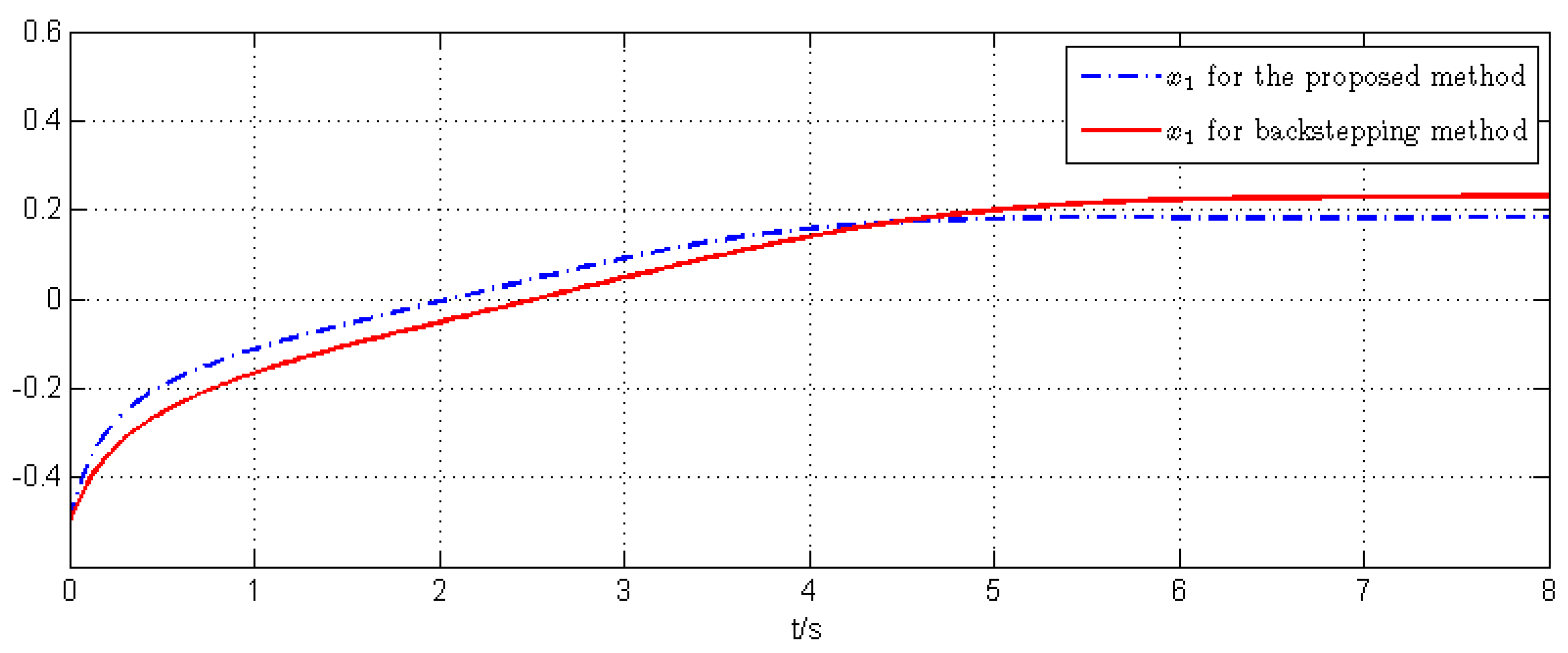
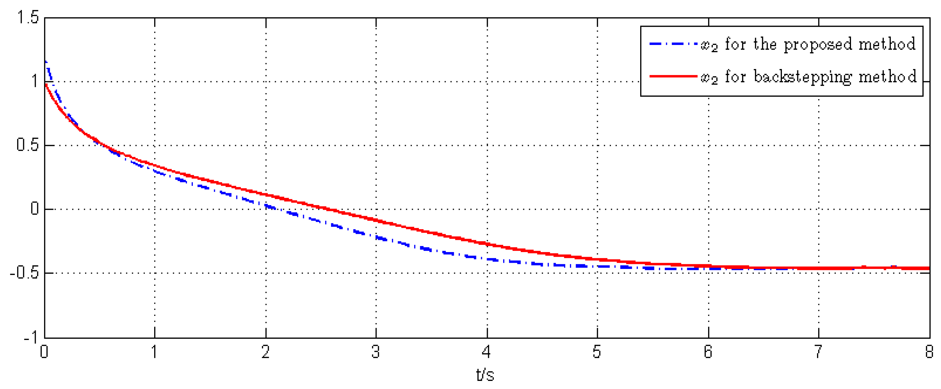
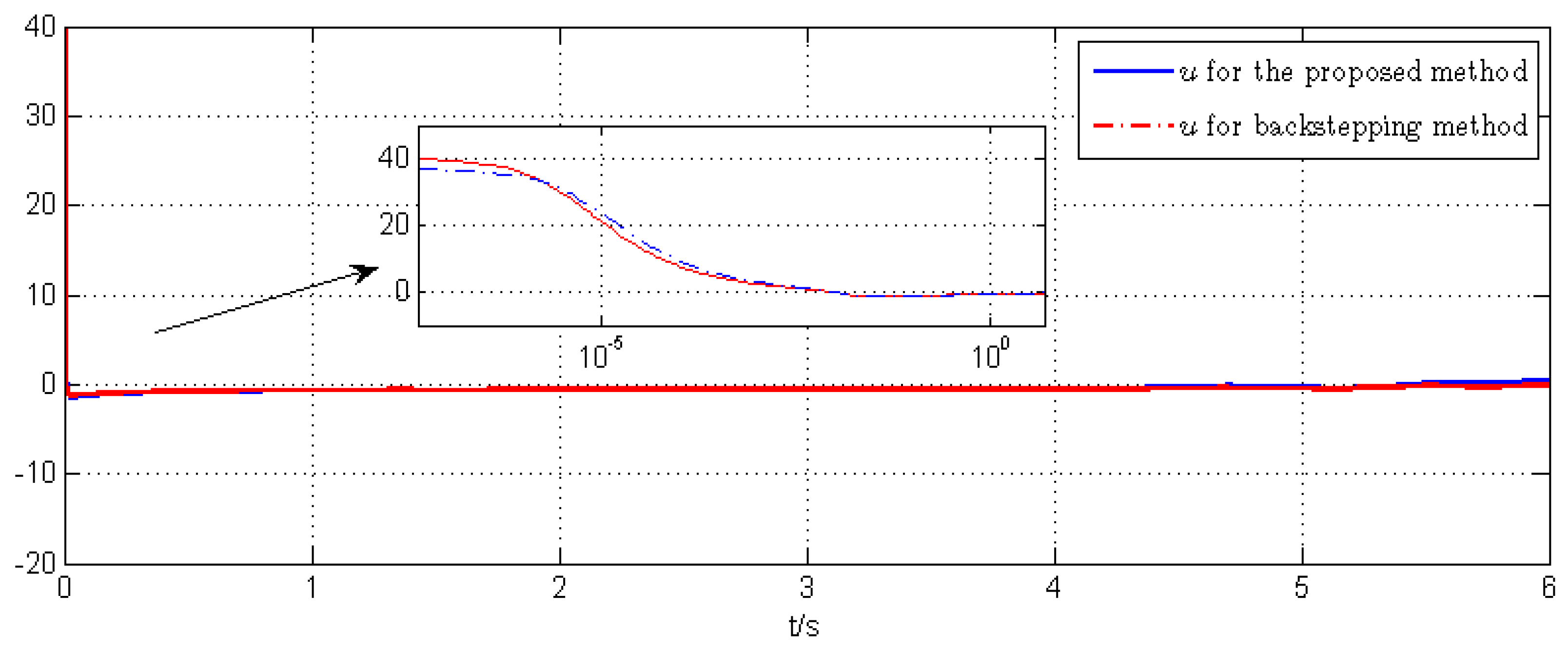
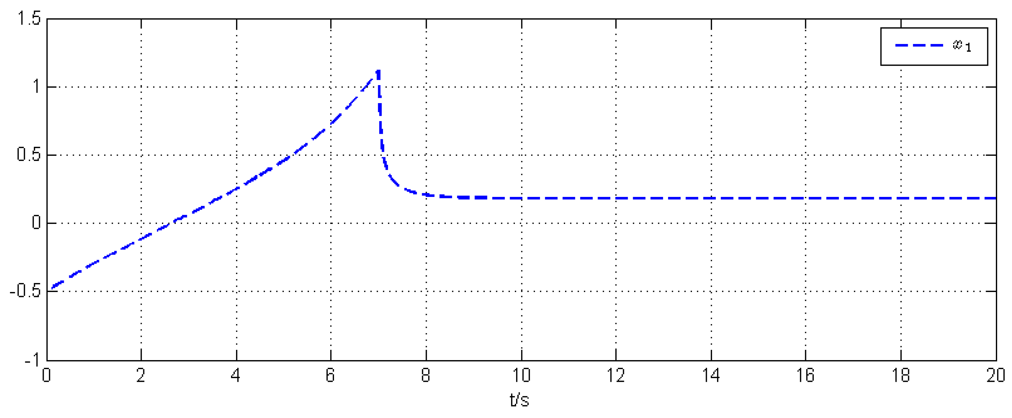
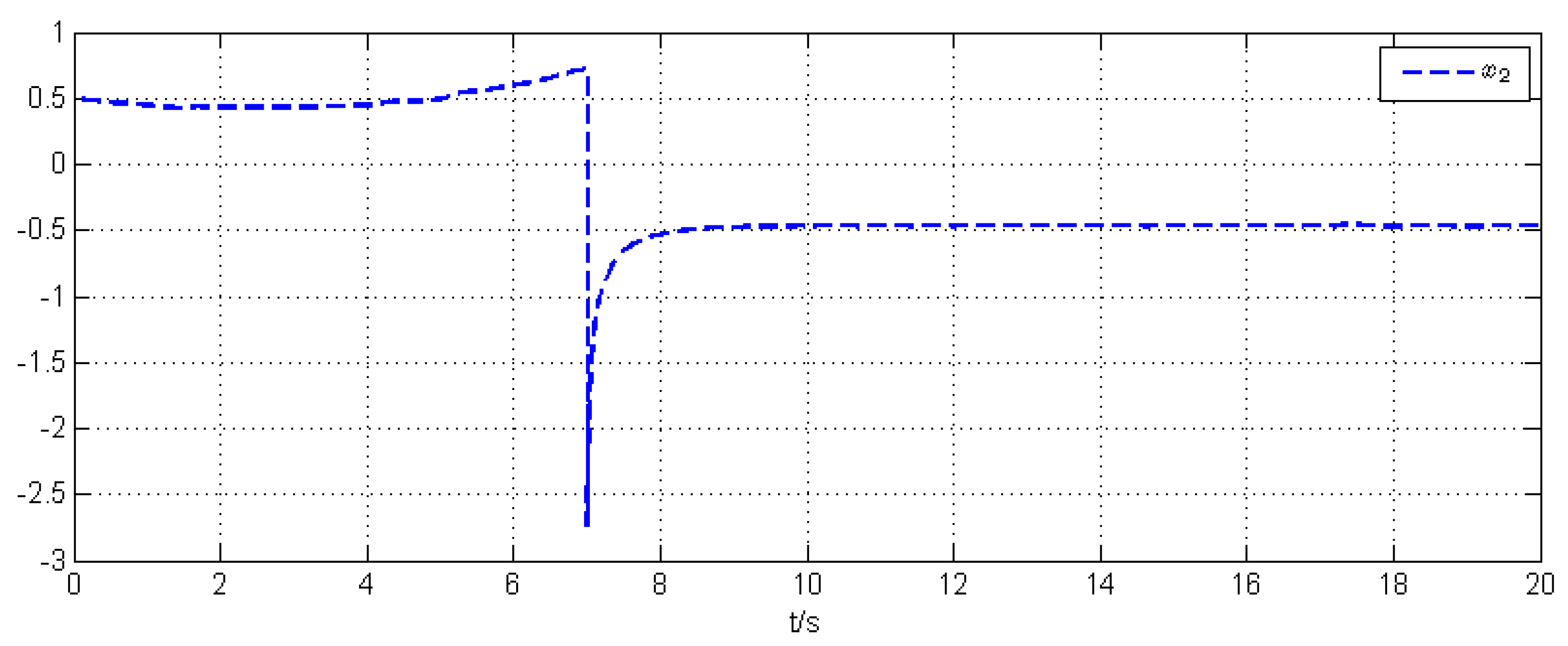
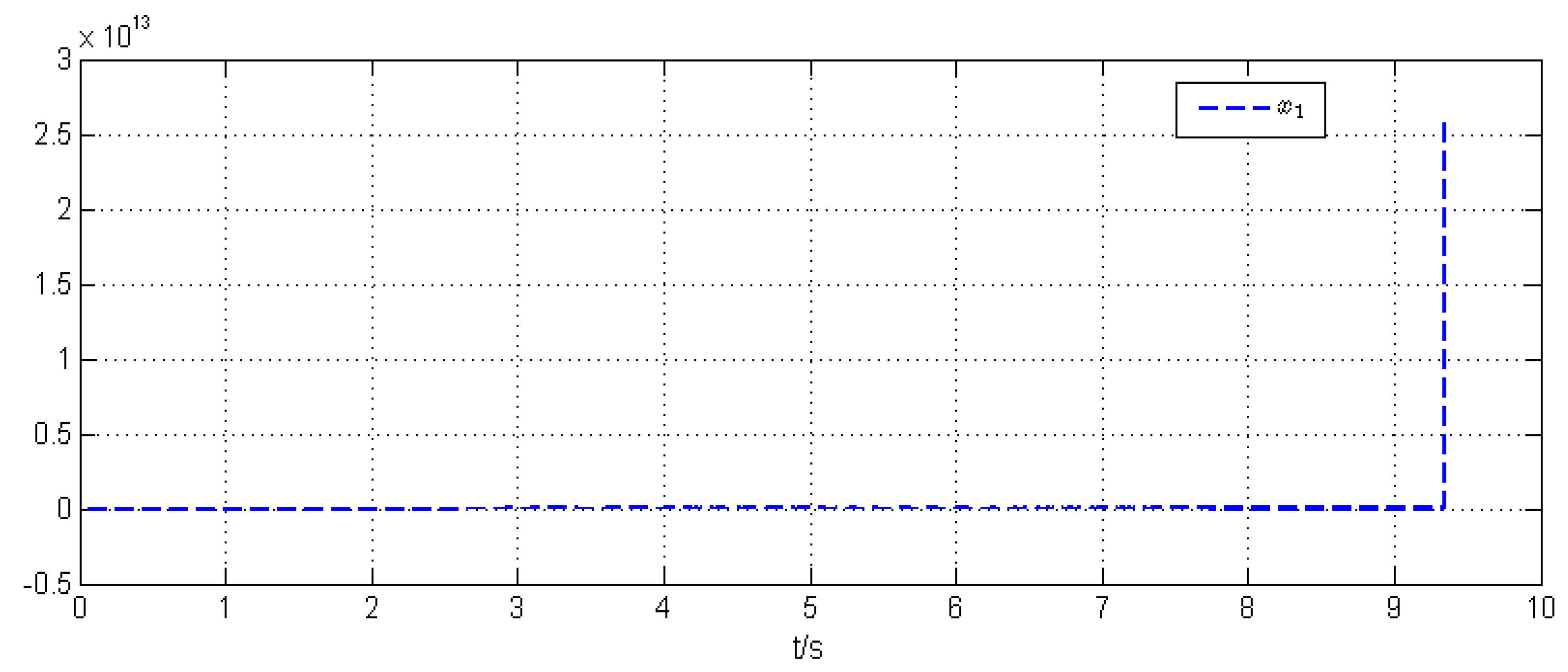
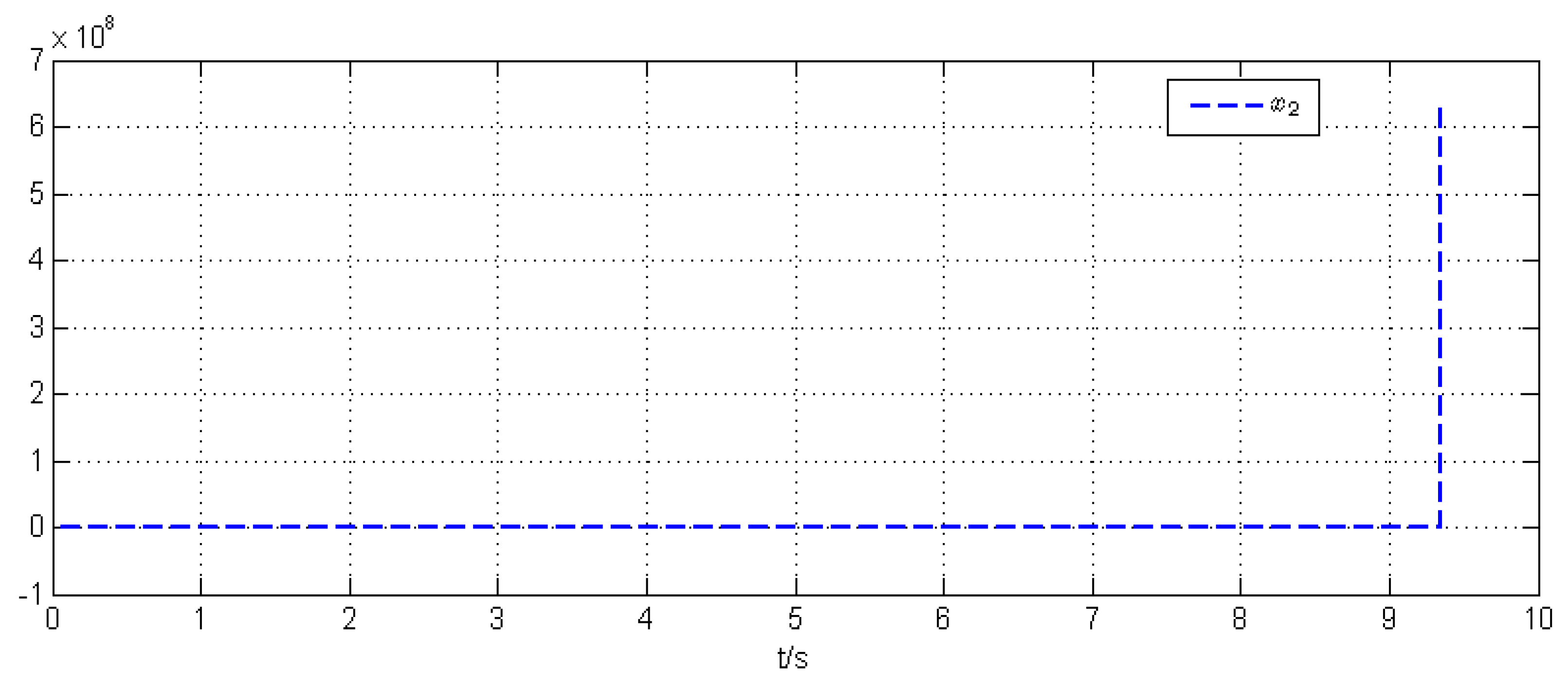
5. Simulation Example

Consider the following system

$$\left\{\begin{array}{l}\mathrm{d}{x}_1=(x_2^3+f_1(x_1))\mathrm{d}t+g_1(x_1)\mathrm{d}w,\hfill \\ \mathrm{d}{x}_2=(u^3+f_2(x))\mathrm{d}t+g_2(x)\mathrm{d}w.\hfill \end{array}\right.$$

where $x_1,x_2$ are system states and $u$ is the control input. In this example, the functions are selected as $f_1=1/10,g_1=0,f_2=1/4x_2{x}_1,g_2(x)=\frac{x_1\sin t}{4+4x_1^2}.$ It shows that Assumption 1 holds. By using the strategy in Section 4, we construct the dynamic-gain-based controller $u=-a^{{\epsilon }_3}(t){\beta }_2{\chi }_2(z)$, $\dot{a}(t)=\frac{c_1}{2c_2}({\displaystyle \sum _{j=1}^2{\psi }_j}(z))\max \{\frac{2c_3}{c_1}{a}^{2-s}(t)-a^2(t),0\},$ where the functions are ${\chi }_1(z)=z_1=\frac{x_1}{a^{{\epsilon }_1}(t)},$ ${\chi }_2(z)=z_2+{\beta }_1{z}_1=\frac{x_2}{a^{{\epsilon }_2}(t)}+{\beta }_1\frac{x_1}{a^{{\epsilon }_1}(t)},$ ${\psi }_1(z)=1,$ ${\psi }_2(z)={\displaystyle \sum _{j=1}^2{\chi }_j^{p-1}}(z).$

In the example, we employ Malab 7.11.0(R2010b) software and use the Simulation part. The parameters are chosen as ${\epsilon }_1=1/3, {\epsilon }_2=4/9, {\epsilon }_3=13/27,$ ${\beta }_2=2, {\beta }_2=50,$$c_1=\frac{1}{2},$$c_2=1/4,c_3=2$. The initial values are$a(0)=5,x_1(0)=-0.5,x_2(0)=0.5$. In the computational environment, we select the solver as ode23t and relative tolerance is set to $1e^{-4}.$ We utilized the presented controller for the system (see the blue dotted curve). The related system responses are provided in Figure 2, Figure 3, Figure 4 and Figure 5. Specially, in Figure 2, the system state $x_1$ does not possess a periodic or non-periodic motion but behaves in a chaos motion. $x_1$ increases and converges to a constant, which indicates that it has a steady-state behavior. As observed in Figure 3, the state $x_2$ also has a chaos motion, i.e., it experiences a decrease within the initial 5 s and subsequently exhibits a tendency towards steady-state behavior. In Figure 4, we see that the control input is much bigger at the beginning of the control. This is because the system at these times is not stable. After a little while, the amplitude of the controller will decrease and keep a small value. The aforementioned phenomenon implies that the system will be unstable in the absence of control input. However, under the designed controller $u$, the system states continue to change. Notably, after approximately 5 s, the system achieves stability in probability. Figure 5 shows that the dynamic gain will increase and converge to the value 8. It shows that the dynamic gain $a(t)$ does not perform a periodic or non-periodic motion but behaves in a chaos motion. Figure 2, Figure 3, Figure 4 and Figure 5 show that all the system signals are bounded in probability. Moreover, the system states converge into a bounded set in a finite time.

To provide a comparison with the existing method, we also make the simulation using the well-known backstepping control method [26,32]. The responses are given in Figure 2, Figure 3 and Figure 4 (see the read solid-line curve). From Figure 2 and Figure 3, we see that the proposed method guarantees faster convergence speed. In detail, by using the proposed method, the state $x_1$ converges to a constant at about 4.5 s, which is faster than the speed of the backstepping method (for this method, $x_1$ converges to a constant at about 6.3 s). Additionally, $x_2$ converges to a constant at about 4.8 s under the proposed method. Differently, the backstepping method requires about 6.2 s and is much slower. Figure 4 shows that the amplitude of the proposed controller is a little smaller. It shows that the proposed method has some advantages compared with the backstepping method.

To show how the controller makes the plant more stable, we also plot the results before and after the use of the controller (before the use of the controller means that the system input stays at $u=0$; after the use of the controller means that $u$ has the values as the designed controller in (18)), see Figure 6 and Figure 7. As shown in Figure 6, before the use of the controller (at 0~7 s), the states $x_1$ will increase from −0.5 to 1.2 and have free motion without regulation of the system control input. After the use of the presented controller (7 s later), the control input has values. The state will be driven back and converge to a fixed constant under the designed controller. From Figure 7, we see that the state $x_2$ has a slow motion before the use of the controller (at 0~7 s). During this period, the state $x_2$ is uncontrolled. When the controller is utilized (7 s later), the system input will follow the values as in (18). State $x_2$ will be pulled to −2.7 from 0.5 and subsequently possess a tendency to converge to −0.5. Figure 6 and Figure 7 show that the system will become unstable without the appropriate controller. Moreover, after the use of the designed controller in this paper, the system states are all guaranteed to be stable. In this example, we also plot the results when there is no controller (see Figure 8 and Figure 9). It shows that the states $x_1$ and $x_2$ will tend to infinity if the system has no effect controller. The above simulation shows that the presented strategy is valid.

6. Conclusions

In this article, we studied control problems for a class of stochastic nonlinear systems. First, a new control strategy that uses the dynamic gain and homogeneous domination method is presented in Theorem 1. It guarantees that the closed-loop system is a semi-global finite-time control issue in probability. Then, the presented strategy is applied to a second-order stochastic nonlinear system. By constructing an appropriate Lyapunov function and choosing the suitable dynamic gain, a new dynamic controller can be constructed to guarantee SGFSP for the system. However, there are still some issues that need to be investigated, for instance, when the systems have uncertainties such as unknown parameters, can we present an adaptive control method? Specifically, when the system’s nonlinear functions have unknown parameters, we can estimate their upper bounds using the inequality in Lemma 1. Then, using the idea of parameter separation in [40], those upper bounds can have a form in which an unknown parameter is multiplied by a known function. A maximum value of unknown parameters that are obtained in the upper bounds of nonlinear functions is defined, and an updated law is designed using an adaptive control method to estimate it. Using the parameter estimation and combining the approach in this paper, we can finally design the adaptive controller. Future work will focus on these issues.

References

1. Lv, L.N.; Sun, Z.Y.; Xie, X.J. Adaptive control for high-order time-delay uncertain nonlinear system and application to chemical reactor system. Int. J. Adapt. Control Signal Process. 2015, 29, 224–241. [Google Scholar] [CrossRef]
2. Sun, W.; Diao, S.Z.; Su, S.F.; Wu, Y.Q. Adaptive fuzzy tracking for flexible-joint robots with random noises via command filter control. Inform. Sci. 2023, 575, 116–132. [Google Scholar] [CrossRef]
3. Zhang, Z.C.; Gao, Y.; Bian, J.S.; Wu, Y.Q. Event-triggered fixed-time tracking of state-constrained surface ships under actuation saturation with prescribed control performance. Ocean Eng. 2023, 281, 114784. [Google Scholar] [CrossRef]
4. Khalil, H.K. Nonlinear Systems, 3rd ed.Prentice Hall: Upper Saddle River, NJ, USA, 2002. [Google Scholar]
5. Sastry, S. Nonlinear Systems: Analysis, Stability, and Control; Springer Science & Business Media: Berlin/Heidelberg, Germany, 2013. [Google Scholar]
6. Mao, X. Stochastic Differential Equations and Applications; Elsevier: Amsterdam, The Netherlands, 2007. [Google Scholar]
7. Do, K.D. Global robust adaptive path-tracking control of underactuated ships under stochastic disturbances. Ocean Eng. 2016, 111, 267–278. [Google Scholar] [CrossRef]
8. Cui, M.Y.; Wu, Z.J.; Xie, X.J. Output feedback tracking control of stochastic Lagrangian systems and its application. Automatica 2014, 50, 1424–1433. [Google Scholar] [CrossRef]
9. Li, W.Q.; Krstic, M. Prescribed-time output-feedback control of stochastic nonlinear systems. IEEE Trans. Autom. Control. 2023, 68, 1431–1446. [Google Scholar] [CrossRef]
10. Cui, R.H.; Xie, X.J. Adaptive state-feedback stabilization of state-constrained stochastic high-order nonlinear systems. Sci. China Inform. Sci. 2021, 64, 1–11. [Google Scholar] [CrossRef]
11. Wang, H.Q.; Liu, P.X.; Bao, J.L.; Xie, X.J.; Li, S. Adaptive neural output-feedback decentralized control for largescale nonlinear systems with stochastic disturbances. IEEE Trans. Neural Netw. Learn. Syst. 2020, 31, 972–983. [Google Scholar] [CrossRef]
12. Sun, Z.Y.; Shao, Y.; Chen, C.C. Fast finite-time stability and its application in adaptive control of high-order nonlinear system. Automatica 2019, 106, 339–348. [Google Scholar] [CrossRef]
13. Chen, C.C.; Sun, Z.Y. A unified approach to finite-time stabilization of high-order nonlinear systems with an asymmetric output constraint. Automatica 2020, 111, 108581. [Google Scholar] [CrossRef]
14. Shao, Y.; Xu, S.Y.; Chen, X.; Zhang, B. Fast finite-time control for a class of stochastic low-order nonlinear system with uncertainties. J. Franklin Inst. 2024, 361, 106788. [Google Scholar] [CrossRef]
15. Yan, Z.G.; Zhang, G.S.; Wang, J.K.; Zhang, W.H. State and output feedback finite-time guaranteed cost control of linear Itô stochastic systems. J. Syst. Sci. Complex. 2015, 28, 813–829. [Google Scholar] [CrossRef]
16. You, Z.Y.; Wang, F. Adaptive fast finite-time fuzzy control of stochastic nonlinear systems. IEEE Trans. Fuzzy Syst. 2022, 30, 2279–2288. [Google Scholar] [CrossRef]
17. Xia, J.W.; Li, B.M.; Su, S.F.; Sun, W.; Shen, H. Finite-time command filtered event-triggered adaptive fuzzy tracking control for stochastic nonlinear systems. IEEE Trans. Fuzzy Syst. 2021, 29, 1815–1825. [Google Scholar] [CrossRef]
18. Lei, H.; Lin, W. Robust control of uncertain systems with polynomial nonlinearity by output feedback. Int. J. Robust Nonlin. Control 2009, 19, 692–723. [Google Scholar] [CrossRef]
19. Wang, T.; Luo, X.; Li, W. Razumikhin-type approach on state feedback of stochastic high-order nonlinear systems with time-varying delay. Int. J. Robust Nonlin. Control 2017, 27, 3124–3134. [Google Scholar] [CrossRef]
20. Min, H.; Xu, S.; Li, Y.; Chu, Y.; Wei, Y.; Zhang, Z. Adaptive finite-time control for stochastic nonlinear systems subject to unknown covariance noise. J. Franklin Inst. 2018, 355, 2645–2661. [Google Scholar] [CrossRef]
21. Sui, S.; Chen, C.L.P.; Tong, S. Finite-time adaptive fuzzy prescribed performance control for high-order stochastic nonlinear systems. IEEE Trans. Fuzzy Syst. 2021, 30, 2227–2240. [Google Scholar] [CrossRef]
22. Sun, J.; He, H.; Yi, J.; Pu, Z. Finite-time command-filtered composite adaptive neural control of uncertain nonlinear systems. IEEE Trans. Cybern. 2020, 52, 6809–6821. [Google Scholar] [CrossRef]
23. Li, W.; Yao, X.; Krstić, M. Adaptive-gain observer-based stabilization of stochastic strict-feedback systems with sensor uncertainty. Automatica 2020, 120, 109112. [Google Scholar] [CrossRef]
24. Wei, X.J.; Wu, Z.J.; Karimi, H.R. Disturbance observer-based disturbance attenuation control for a class of stochastic systems. Automatica 2016, 63, 21–25. [Google Scholar] [CrossRef]
25. Su, H.; Zhang, W. Adaptive fuzzy control of stochastic nonlinear systems with fuzzy dead zones and unmodeled dynamics. IEEE Trans. Cybern. 2018, 50, 587–599. [Google Scholar] [CrossRef] [PubMed]
26. Deng, H.; Krstić, M. Stochastic nonlinear stabilization—I: A backstepping design. Syst. Control Lett. 1997, 32, 143–150. [Google Scholar] [CrossRef]
27. Sun, Y.; Chen, B.; Lin, C.; Wang, H.; Zhou, S. Adaptive neural control for a class of stochastic nonlinear systems by backstepping approach. Inform. Sci. 2016, 369, 748–764. [Google Scholar] [CrossRef]
28. Xia, M.; Zhang, T. Adaptive neural dynamic surface control for full state constrained stochastic nonlinear systems with unmodeled dynamics. J. Franklin Inst. 2019, 356, 129–146. [Google Scholar] [CrossRef]
29. Xia, X.; Zhang, T.; Zhu, J.; Yi, Y. Adaptive output feedback dynamic surface control of stochastic nonlinear systems with state and input unmodeled dynamics. Int. J. Adapt. Control Signal Process. 2016, 30, 864–887. [Google Scholar] [CrossRef]
30. Liu, S.; Niu, B.; Zong, G.; Zhao, X.; Xu, N. Adaptive neural dynamic-memory event-triggered control of high-order random nonlinear systems with deferred output constraints. IEEE Trans. Autom. Sci. Eng. 2023. [CrossRef]
31. Tong, D.; Xu, C.; Chen, Q.; Zhou, W.; Xu, Y. Sliding mode control for nonlinear stochastic systems with Markovian jumping parameters and mode-dependent time-varying delays. Nonlinear Dynam. 2020, 100, 1343–1358. [Google Scholar] [CrossRef]
32. Wang, L.; Liu, X.; Xue, X.; Wei, Y.; Li, T.; Chen, X. Backstepping control for stochastic nonlinear strict-feedback systems based on observer with incomplete measurements. Int. J. Control 2022, 95, 3211–3225. [Google Scholar] [CrossRef]
33. Liu, Y.; Liu, X.P.; Jing, Y.W.; Zhang, Z.Y. Semi-globally practical finite-time stability for uncertain nonlinear systems based on dynamic surface control. Int. J. Control 2021, 94, 476–485. [Google Scholar] [CrossRef]
34. Spelta, A.; Pecora, N.; Pagnottoni, P. Chaos based portfolio selection: A nonlinear dynamics approach. Expert Syst. Appl. 2022, 188, 116055. [Google Scholar] [CrossRef]
35. Jhangeer, A.; Almusawa, H.; Hussain, Z. Bifurcation study and pattern formation analysis of a nonlinear dynamical system for chaotic behavior in traveling wave solution. Results Phys. 2022, 37, 105492. [Google Scholar] [CrossRef]
36. Song, Z.; Zhai, J. Practical output tracking control for switched nonlinear systems: A dynamic gain based approach. Nonlinear Anal. Hybrid Syst. 2018, 30, 147–162. [Google Scholar] [CrossRef]
37. Cheng, X.; Liu, Z.; Zhang, L. Small perturbations may change the sign of Lyapunov exponents for linear SDEs. Stoch. Dyn. 2022, 22, 2240038. [Google Scholar] [CrossRef]
38. Luo, S.; Deng, F. Necessary and sufficient conditions for 2pth moment stability of several classes of linear stochastic systems. IEEE Trans. Autom. Control 2019, 65, 3084–3091. [Google Scholar] [CrossRef]
39. Ling, Q.; Jin, X.; Wang, Y.; Li, H.F.; Huang, Z.L. Lyapunov function construction for nonlinear stochastic dynamical systems. Nonlinear Dynam. 2013, 72, 853–864. [Google Scholar] [CrossRef]
40. Lin, W.; Qian, C. Adaptive control of nonlinearly parameterized systems: A nonsmooth feedback framework. IEEE Trans. Autom. Control 2002, 47, 757–774. [Google Scholar] [CrossRef]
Figure 1. The diagram of the control strategy.
Processes 12 01377 g001
Figure 2. Trajectory of state x 1 .
Processes 12 01377 g002
Figure 3. Trajectory of state x 2 .
Processes 12 01377 g003
Figure 4. Trajectory of the control input u .
Processes 12 01377 g004
Figure 5. Trajectory of the dynamic gain a ( t ) .
Processes 12 01377 g005
Figure 6. Trajectory of state x 1 before and after use of the controller.
Processes 12 01377 g006
Figure 7. Trajectory of state x 2 before and after use of the controller.
Processes 12 01377 g007
Figure 8. Trajectory of state x 1 without the system input u .
Processes 12 01377 g008
Figure 9. Trajectory of state x 2 without the system input u .
Processes 12 01377 g009
Disclaimer/Publisher’s Note: The statements, opinions and data contained in all publications are solely those of the individual author(s) and contributor(s) and not of MDPI and/or the editor(s). MDPI and/or the editor(s) disclaim responsibility for any injury to people or property resulting from any ideas, methods, instructions or products referred to in the content.