Research on an Adaptive Active Suspension Leveling Control Method for Special Vehicles

Abstract

Adaptive active suspension systems, integral to specialized vehicles, hold significance for their stability and safety. This study introduces a novel adaptive active suspension system featuring four independently controlled wheels employing wheel-hub motors, hydraulic cylinders, pump motor power, controllers, and sensors. A rapid and, within a certain range, leveling and height adjustment control strategy is proposed for this system, utilizing the Kalman filter algorithm. Additionally, the paper examines the front-wheel Ackermann steering model and four-wheel reverse Ackermann transition model to enhance the suspension’s stability. Subsequently, experiments on leveling and height adjustment are conducted, demonstrating the system’s capability to swiftly and accurately rectify the vehicle’s deviation angle within the specified threshold. Following adjustments made by the leveling and height control algorithm, the vehicle body promptly returns to the preset level state and designated height. The leveling control system holds broad applicability in intelligent agriculture, logistics handling, off-road equipment, and other domains, presenting significant practical utility.

1. Introduction

Special vehicles, tailored for specific fields or tasks, such as emergency rescue vehicles [1], intelligent weapon vehicles [2], field medical vehicles [3], and vehicles for intelligent agriculture [4], often integrate numerous high-precision output devices. Prior to the operation of such devices, it is essential for the vehicle platform to maintain a specified height with stable horizontal plane characteristics, facilitating the execution of various complex actions by vehicle-mounted equipment. The precision of the vehicle platform’s leveling upon arrival at the task site is a critical technical parameter, significantly impacting the performance and stability of special vehicles. Thus, incorporating an active suspension system with leveling and height adjustment capabilities holds paramount importance in enhancing the performance of special vehicles and broadening their scope of application.

Insufficient literature exists regarding the airport special vehicle count [5]. Inadequate scheduling can severely impair airport service efficiency, posing a significant challenge. To address this issue, a dual-objective mixed-integer programming model is proposed, aiming to optimize scheduling. Additionally, a genetic algorithm is devised to tackle the integrated scheduling problems efficiently.

A study [6] discussed traffic congestion issues encountered by special vehicles during urgent tasks and proposed a blockchain-based scheme to prioritize access for these vehicles, ensuring real-time scheduling and priority. The power output system of special vehicles represented by new energy is often used as the power source of torque output by the hub motor. The motors in the hub motor are permanent-magnet synchronous motors, which have the advantages of simple structure, light weight, high power density, and high efficiency [7,8,9] and are used to achieve the traveling action of the active suspension. The study [7] developed a predictive functional control (PFC) method and applied it to the speed controller of permanent-magnet synchronous motors, which improved the speed control accuracy of permanent-magnet synchronous motors. Reference [8] adopted the SMC method to improve the robustness of the system. Reference [9] applied the fuzzy logic control method to the permanent-magnet synchronous motor control system of electric vehicles, which can effectively solve the problem of sudden load speed changes in permanent-magnet synchronous motors.

Another study [10] systematically introduced the characteristics of wheel-hub motor drive systems commonly used in special vehicles on different occasions, described the key technical problems of wheel-hub motor applications in special vehicles, and analyzed the development trend of wheel-hub motors in special vehicles. In another study [11], to improve the fault tolerance of wheel-hub motors in special vehicles, a robust optimization method based on fuzzy control was proposed, and the feasibility and effectiveness of the method were verified. Two methods, the sequential quadratic programming (SQP) algorithm and the NSGA-II algorithm, were proposed for the design optimization of permanent-magnet synchronous motors (PMSMs) in wheel-hub motor applications in special vehicles, and the most suitable optimization scheme was selected [12]. Dai et al. [13] addressed the problem of performance optimization of permanent-magnet synchronous motor (PMSM) drives for special vehicles and successfully solved the problem of drive performance optimization by analyzing the impact of key parameters on performance, achieving the required torque-speed characteristics, and improving traction performance and supply quality. Kim et al. [14] proposed a solution based on a novel sliding mode observer (SMO) for the sensorless speed control problem of a permanent-magnet synchronous motor (PMSM), which introduced a high-speed SMO to estimate the rotor position and angular velocity and improved the steady-state performance of the system.

For the speed control problem of the permanent-magnet synchronous motor (PMSM) servo system, Liu et al. [15] proposed a solution utilizing the predictive function control (PFC) method. The introduction of an improved PFC + extended states observer (ESO) method effectively enhanced system control performance. Conventional suspension systems frequently lack the capability for active leveling and height adjustment when navigating intricate terrain, consequently compromising the accuracy of onboard equipment and potentially jeopardizing overall stability. Hence, the development of an active suspension system featuring active leveling and height adjustment holds immense significance. Such a system is anticipated to enhance vehicle stability and reliability.

This paper presents an innovative adaptive active suspension system that analyzes nine attitudes of the vehicle body based on the attitude of the gyroscope. Through different adjustment strategies, the vehicle body can be in a horizontal state within a certain range and can achieve forward, backward, diagonal, lateral, and Ackermann steering of the vehicle at different speeds.

An automatic leveling and height adjustment control strategy is proposed in this study, incorporating hydraulic cylinders, gyroscopes, and displacement sensors. This system actively adjusts the suspension’s height and attitude based on the vehicle’s actual driving conditions and terrain, ensuring consistent stability and precision of the vehicle platform. Consequently, the flexibility and stability of the adaptive active suspension are significantly enhanced. Furthermore, this system serves as a valuable reference for designing and leveling other specialized vehicles. With ongoing technological advancements and expanding application domains, this active and advanced adaptive suspension is poised to play a crucial role in enabling future special vehicles to undertake a diverse range of complex tasks.

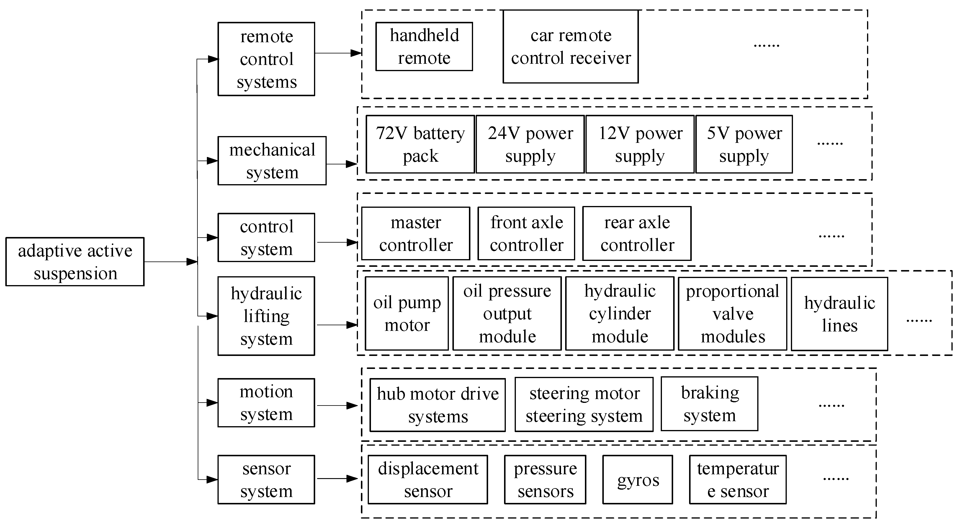
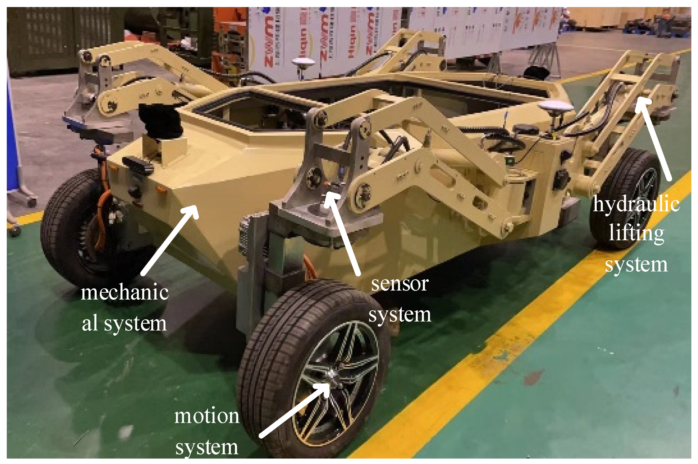
2. Adaptive Active Suspension System Components

This adaptive active suspension system is mainly composed of six parts: a remote control part, a power part, a control part, a hydraulic lift part, a motion part, and a sensing part. The structural composition of these six parts is shown in Figure 1.

The structure of the adaptive active suspension is shown in Figure 2.

The adaptive active suspension employs a CAN communication mode, renowned for its robust anti-disturbance properties, minimal signal degradation, and stable interconnection among diverse sensors, controllers, and actuators.

Upon receiving the command from the handheld remote control, the vehicle’s remote-control receiver relays it to the central controller via CAN communication. Subsequently, the central controller interprets the command and orchestrates the active suspension to execute the designated action.

The active suspension operates using a 72 V high-efficiency battery pack. Through voltage conversion, the power supply system generates 24 V, 12 V, and 5 V outputs to power the sensors, controllers, lighting system, and other components throughout the suspension system.

The control system is primarily composed of the total controller, front axle controller, and rear axle controller. To ensure the active suspension system’s reliability, distinct front axle and rear axle controllers are implemented. The total controller receives signals from various sensors as well as from the front and rear axle controllers. The front axle controller is responsible for managing the steering, brakes, and hub motors of the front axle portion of the active suspension, while the rear axle controller oversees the steering, brakes, and hub motors of the rear axle portion of the active suspension.

The hydraulic lift system is mainly composed of an oil pump motor, a hydraulic cylinder, a hydraulic output module, and a hydraulic pipeline. The hydraulic lifting system is the key to active suspension leveling, and the hydraulic lifting part is installed in the wheel-leg position of the active suspension and plays the role of fixed support. By controlling the extension and retraction positions of the four hydraulic cylinders, the height adjustment and leveling of the active suspension can be realized.

The motion segment primarily includes the drive system, steering system, and brake system. The drive system is predominantly composed of hub motors. The steering system comprises four fully autonomous steering motors, enabling individual steering of each wheel to specific angles. The two front steering systems cooperate for front-wheel Ackermann steering, while the two rear steering systems collaborate for rear-wheel Ackermann steering. This coordination among the four wheel assemblies facilitates four-wheel Ackermann steering.

The sensing system plays a pivotal role in enabling height and leveling functions within the adaptive active suspension. It primarily comprises displacement sensors, pressure sensors, gyroscopes, temperature sensors, and similar components. Displacement sensors are primarily employed to measure the ground height of the active suspension, facilitating height adjustment. Pressure sensors measure the oil pressure within the hydraulic system. Gyroscopes primarily aid in adjusting the body’s attitude, ensuring horizontal alignment. Temperature sensing is chiefly utilized to monitor the temperature of the wheel motors, steering motors, and oil pump motors, preventing potential damage due to excessive heat.

3. Adaptive Active Suspension Leveling

The body of the adaptive active suspension system is supported by four independent wheel legs, each of which contains a set of mutually independent hydraulic cylinders. By adjusting the extension and contraction distance of the hydraulic cylinders, the height of the wheel legs can be adjusted, and then the ground clearance of the active suspension can be adjusted. The adjustable range of the active suspension height from the ground is approximately 30 cm to 1500 cm, and within a certain range, control of the hydraulic cylinder extension and contraction distance is the key to realizing active suspension height adjustment and leveling.

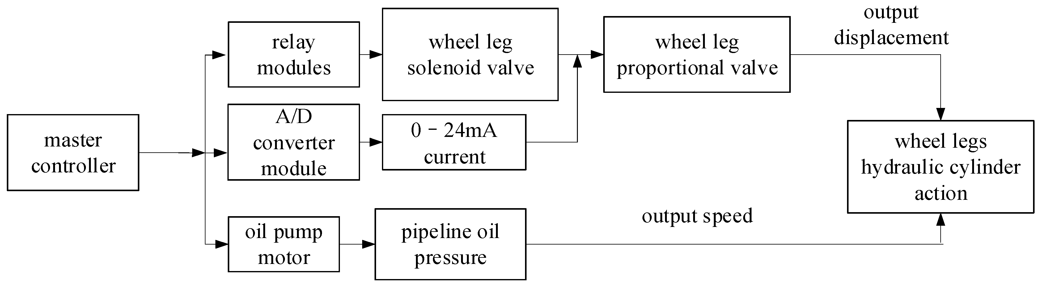
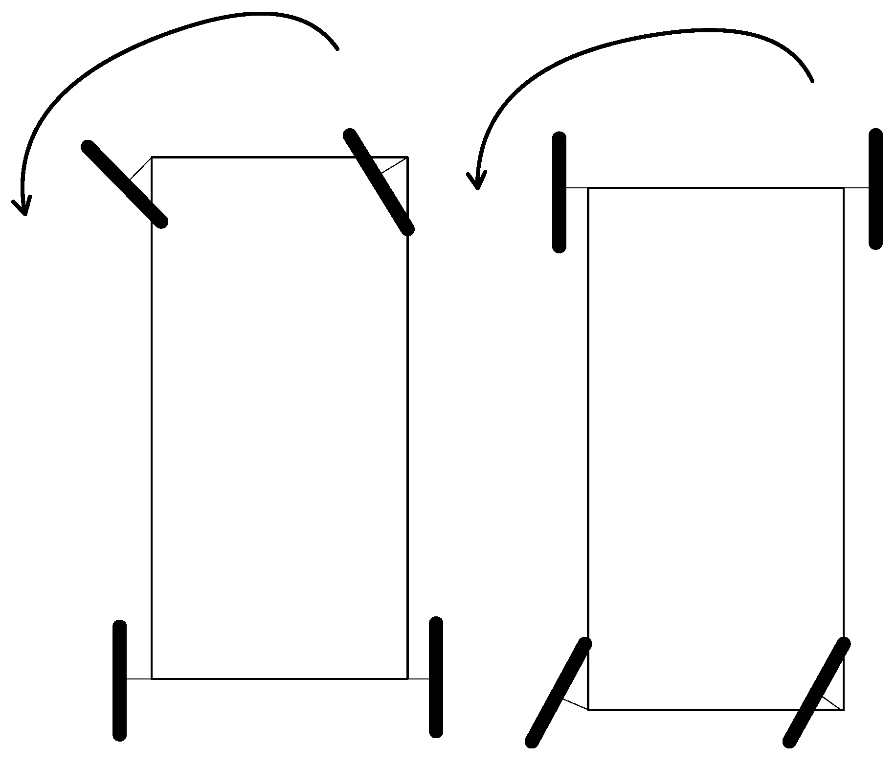
3.1. Wheel-Leg Hydraulic Cylinder Principle of Action

The four hydraulic cylinders for each wheel leg operate independently, allowing control strategies for one cylinder to apply seamlessly to the others. Upon receiving a signal from the remote controller, the controller initiates the control process for the wheel-leg hydraulic cylinder. Initially, the oil pump motor is activated to supply hydraulic pressure to the system, followed by the opening of the solenoid valve to regulate the hydraulic cylinder. The controller adjusts the output current size via the A/D converter module, directly influencing the proportional valve and controlling the hydraulic cylinder’s displacement. The magnitude of the oil pressure from one of the oil pump motors mainly impacts the speed of the hydraulic cylinder’s movement. Conversely, the control volume of the proportional valve primarily determines the displacement of the hydraulic cylinder. For example, if the control volume of the proportional valve is set between 0–20 mA, the hydraulic cylinder extends from 0 to its maximum value.

The total controller governs the extension and contraction of a single hydraulic cylinder, as depicted in Figure 3.

The response rate of the wheel-leg hydraulic cylinder directly impacts the speed of height adjustment and leveling for the vehicle. Given the diverse load distribution across the body, each of the four hydraulic cylinders exhibits distinct characteristics. Even when subjected to the same hydraulic pressure and control commands, the extension and contraction displacements of the four hydraulic cylinders differ. To ensure uniformity in the lifting process of the hydraulic cylinders, a specific ratio coefficient, determined through experimental testing, is applied to the control of each hydraulic cylinder.

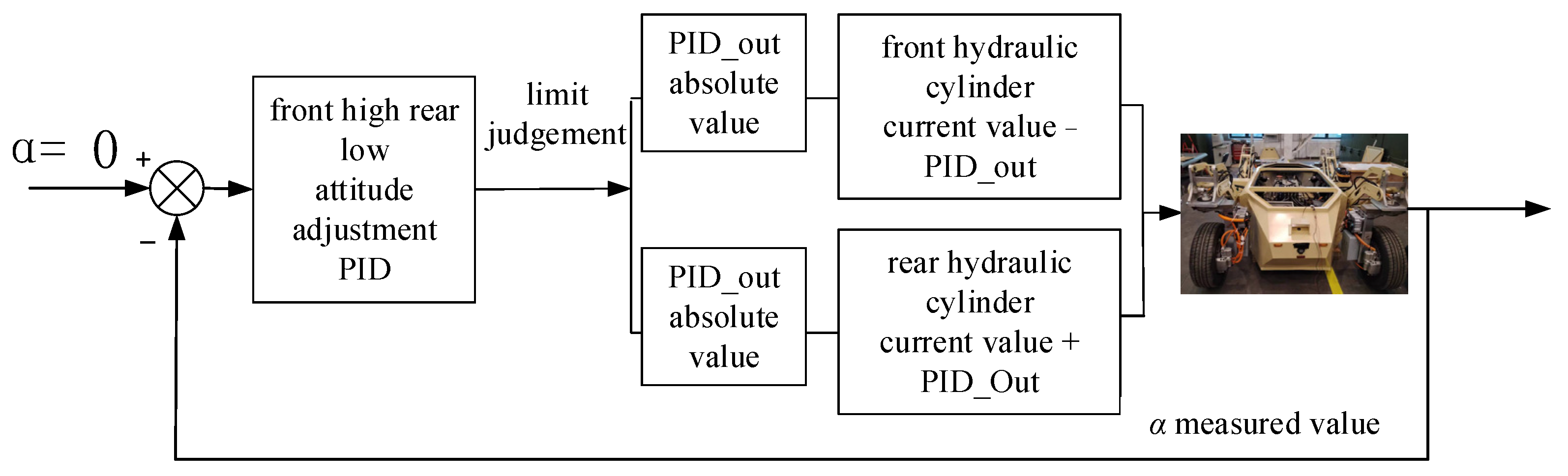
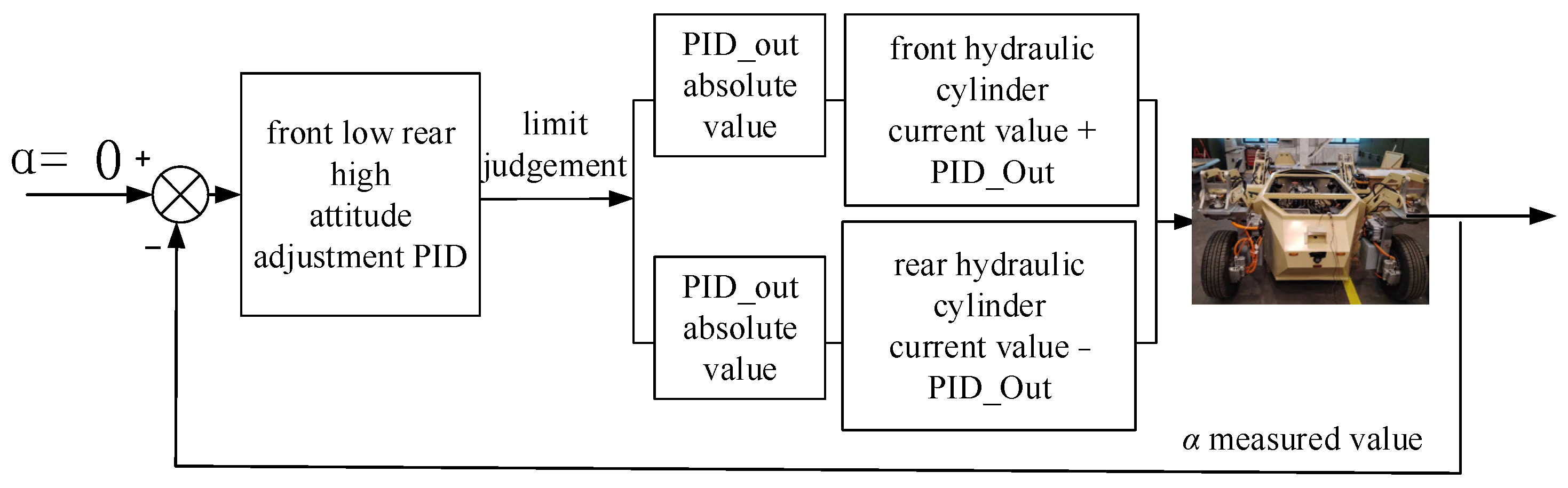
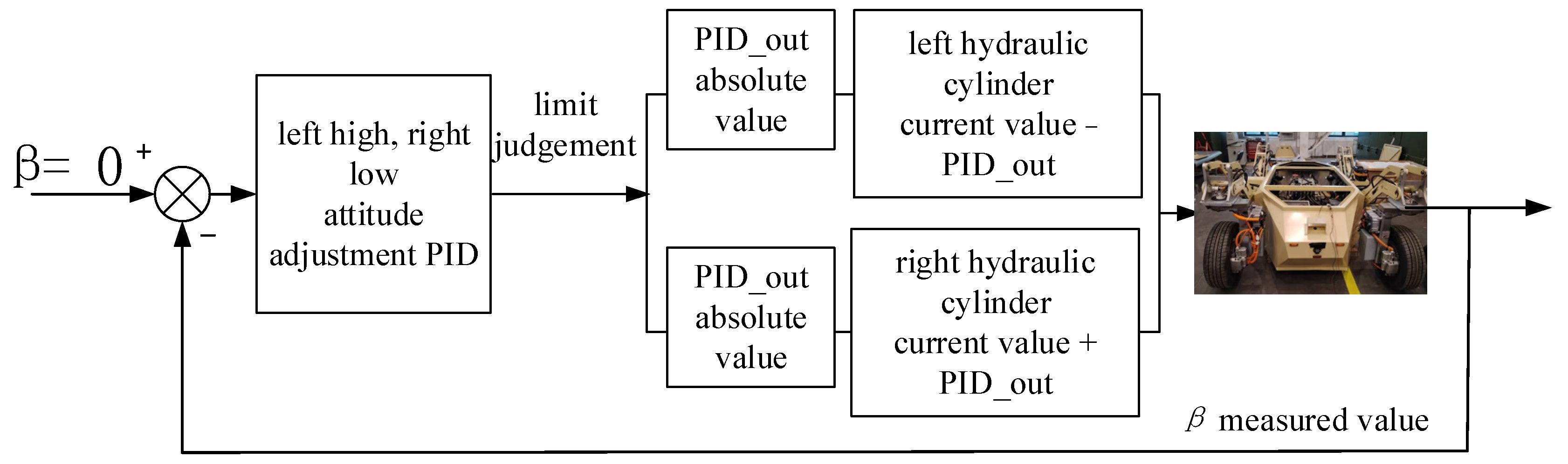
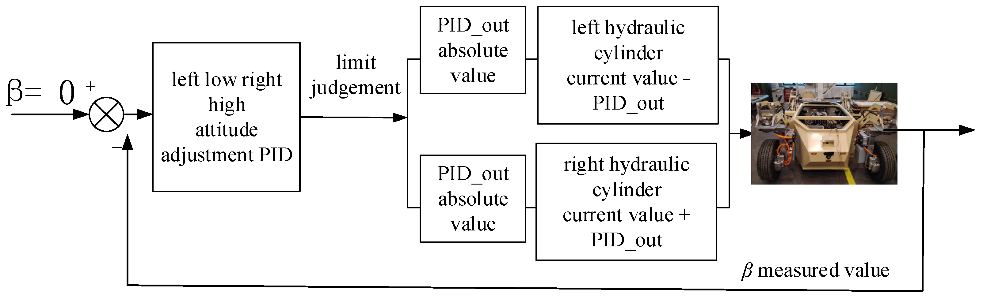
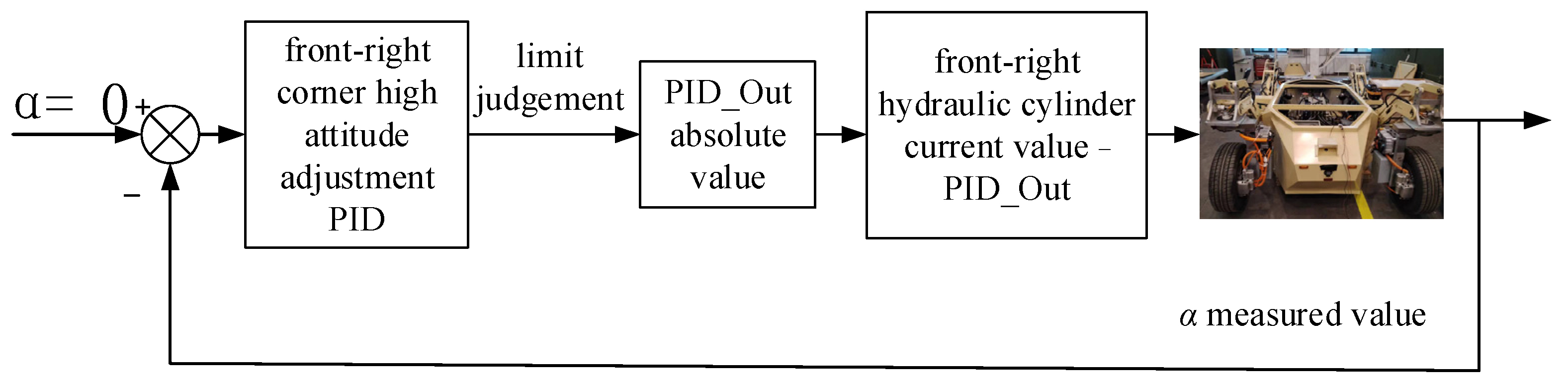
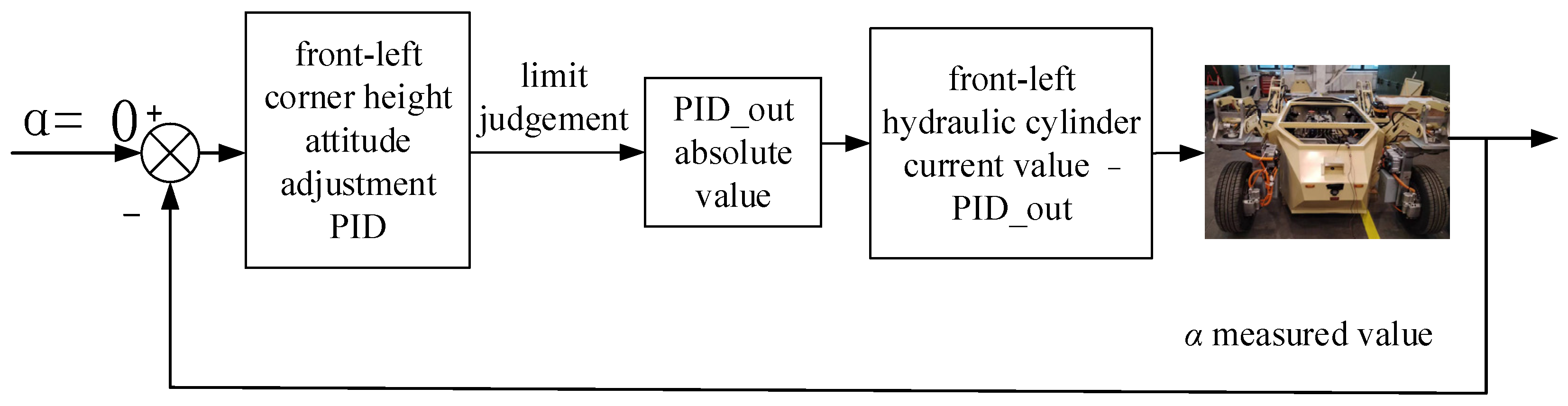
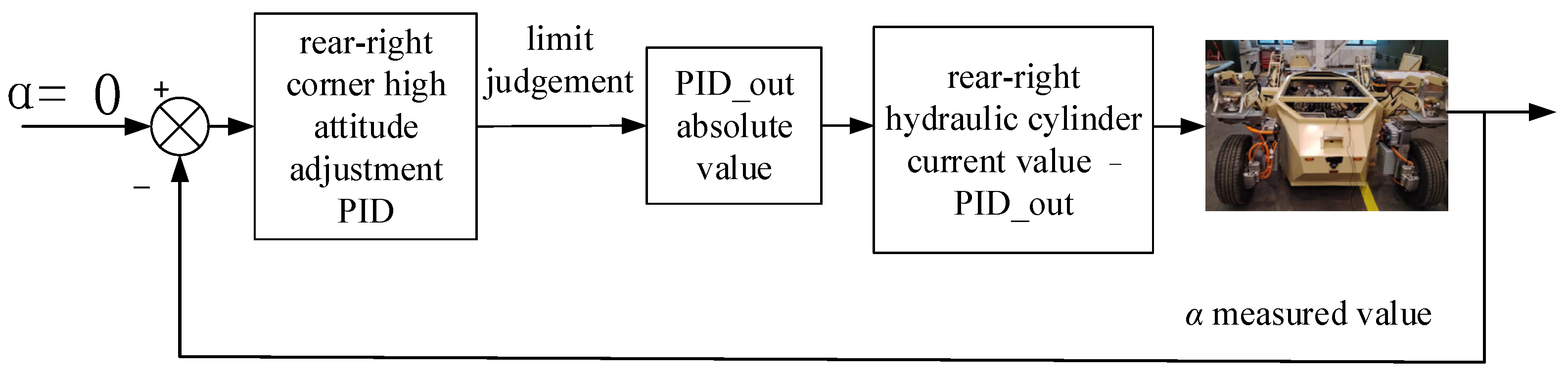
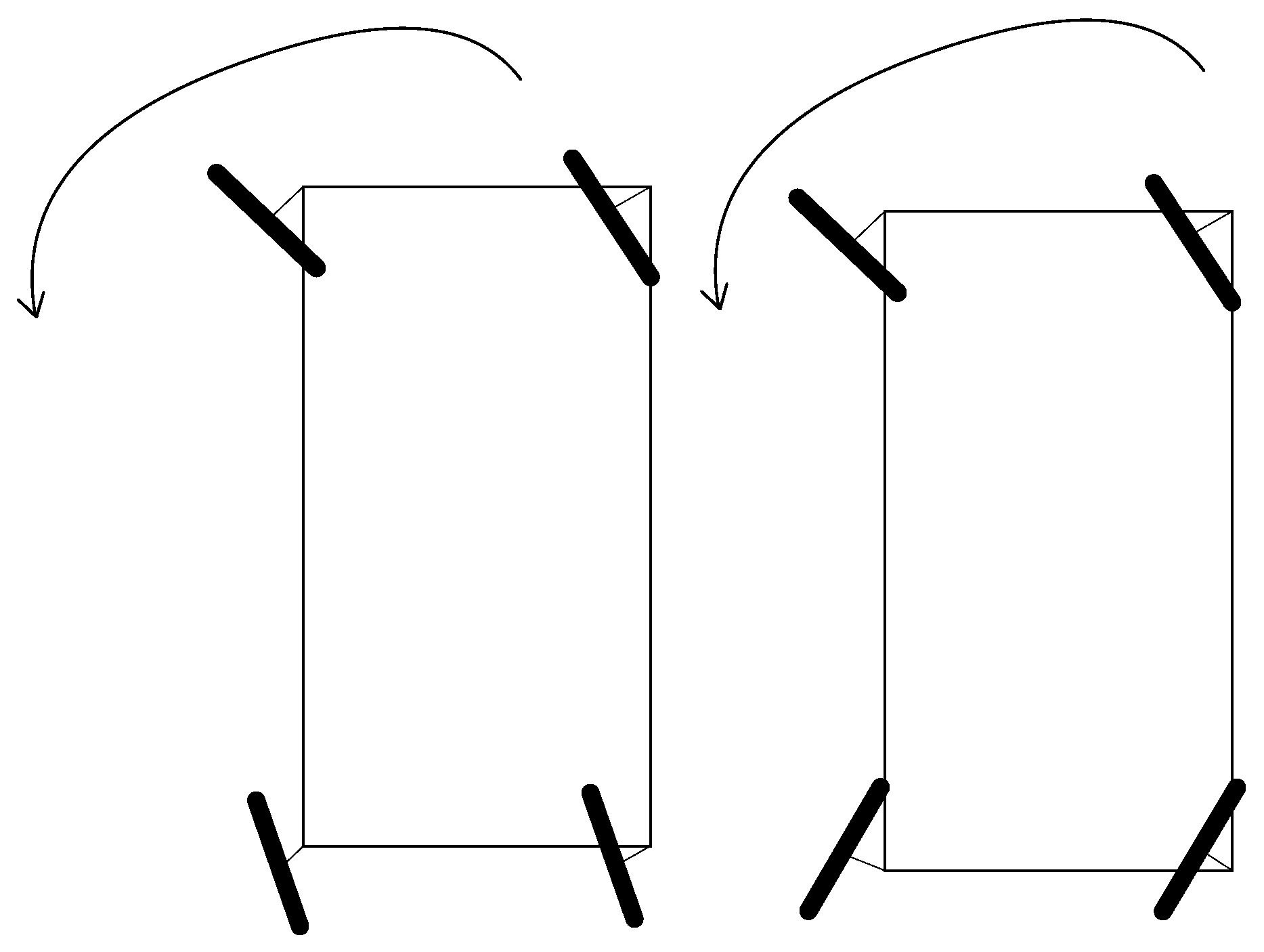
3.2. Adaptive Active Suspension Leveling

To ensure the leveling of the adaptive active suspension’s body, a gyro sensor CH110 is installed at the center of the chassis. This sensor features a compact, low-latency, energy-efficient inertial measurement unit capable of outputting attitude angles at a rate of up to 400 Hz. Using the attitude angle data provided by the gyroscope, the total controller can interpret the current attitude of the active suspension and subsequently make necessary adjustments to maintain the body in a horizontal state.

Based on the gyroscope’s feedback regarding the roll angle and pitch angle, the adaptive active suspension system’s body attitude includes nine positions, including high left front angle, high right front angle, high left rear angle, high right rear angle, high front and low rear, low front and high rear, high left and low right, low left and high right, and horizontal posture. The relationship between the measured body attitude and the gyroscope feedback of the horizontal roll angle α and pitch angle β is depicted in

Table 1. Attitude angle in different states.

Stance	Gyro Feedback Angle
High in front and low at the back (attitude 1)	α > 0, β = 0
Front low/back high (attitude 2)	α < 0, β = 0
Left high/right low (attitude 3)	α = 0, β > 0
Left low/right high (attitude 4)	α = 0, β < 0
Front right angle high (attitude 5)	α > 0, β < 0
Front left angle high (attitude 6)	α > 0, β > 0
Back right angle high (attitude 7)	α < 0, β < 0
Back left angle high (attitude 8)	α < 0, β > 0
Horizontal (attitude 9)	α = 0, β = 0

.

Real-time detection of the gyroscope roll angle and pitch angle data is performed to determine the body in that state.

If the body is in a state of high front/low back, the hydraulic cylinders of the front two wheel legs are adjusted to move downward, and the rear two wheel legs are adjusted to move upward so that the body is in a horizontal state.

If the body is in the front low/back high state, then the front two wheel legs of the hydraulic cylinder are adjusted to move upward, and the rear two wheel legs of the hydraulic cylinder are adjusted to move downward so that the body is in a horizontal state.

If the body is in a high left/low right state, the left two wheel legs are adjusted to move downward, and the right two wheel legs are adjusted to move upward so that the body is in a horizontal state.

If the body is in a low left/high right state, the left two wheel legs are adjusted to move upward, and the right two wheel legs are adjusted to move downward to make the body horizontal.

If the body is in the front right corner high state, then the downward movement of the front right corner wheel-leg hydraulic cylinder is adjusted. In the front right corner wheel-leg hydraulic cylinder downward process, the cylinder may enter the horizontal state, or there may be an expression of one of attitudes 1–4, in which case the appropriate kind of adjustment will occur.

If the body is in the front left corner high state, then the downward movement of the front left corner of the wheel-leg hydraulic cylinder, which is in the front left corner of the wheel-leg hydraulic cylinder descending process, may enter the horizontal state; if the body assumes one of attitudes 1–4, the appropriate kind of adjustment will occur.

When the body is in a raised state at the rear right corner, the hydraulic cylinder of the rear right wheel leg is adjusted downward. During the descent of the hydraulic cylinder at the rear right corner, the body may transition to a horizontal state or assume one of attitudes 1–4. If the latter, adjustments are made to transition the body to the desired state.

When the body is in a raised state at the rear left corner, the hydraulic cylinder of the rear left corner wheel leg is adjusted downward. As the rear left corner wheel-leg hydraulic cylinder descends, the body may transition into a horizontal state, or it may assume one of attitudes 1–4. If the latter, adjustments are made to transition the body to the desired state. Several unbalanced attitudes adjustment processes are shown in Figure 4.

Eight PID controllers have been designed to control the leveling action corresponding to each of the eight non-horizontal attitudes. Given the varying load distribution of the body and the distinct characteristics of the hydraulic cylinders, the PID control parameters for each attitude differ. Therefore, adjustments to the PID control parameters are required based on the specific attitude being addressed.

An expedited controller is utilized to evaluate the present body attitude using the gyroscope and then modify the hydraulic cylinder through proportional valve control to regulate the height of the wheel legs. The control flow diagram is depicted in Figure 5.

When the active suspension system is leveled, the gyroscope attitude is first read according to the information of α and β to determine which attitude the body is in. When the body is in the front high/rear low state, the angle of β is approximately 0 and the angle of α is greater than 0, according to which the state is designed to be adjusted by the PID closed loop. The input of this state is α = 0, and the output of the PID controller acts on the front and rear hydraulic cylinders to make the front two hydraulic cylinders’ wheel legs move downward and the rear two hydraulic cylinders’ wheel legs move upward, adjusting the body attitude to put the body in a horizontal state. The PID closed-loop adjustment of the front high/rear low attitude is shown in Figure 6. The photograph in Figure 6 is a picture of the vehicle. “↑” represents upward movement. “↓” represents downward movement.

When the body assumes a state of front low/rear high, the angle of β is approximately 0, while the angle of α is less than 0. A PID closed-loop adjustment is devised for this condition. The input for this state is set as α = 0, directing the output of the PID controller to elevate the front two hydraulic cylinder wheel legs and depress the rear two hydraulic cylinder wheel legs. This adjustment aims to align the body horizontally. The PID closed-loop adjustment for the front low/rear high attitude is illustrated in Figure 7.

When the body is in a high left/low right state, the angle of α is approximately 0 and the angle of β is more than 0. According to this state, a PID closed-loop adjustment is designed. The input of this state is β = 0, and the output of the PID controller acts on the left and right hydraulic cylinders to make the wheel legs of the left two hydraulic cylinders move downward and the wheel legs of the right two hydraulic cylinders move upward, adjusting the body attitude to put the body in a horizontal state. The PID closed-loop adjustment of the left high/right low attitude is shown in Figure 8.

When the body is in a state of left low/right high, the angle of α is around 0, while the angle of β is less than 0. A PID closed-loop adjustment is tailored for this scenario. The input parameter for this state is set as β = 0, guiding the PID controller’s output to elevate the left two hydraulic cylinder wheel legs and lower the right two hydraulic cylinder wheel legs. This adjustment aims to orient the body horizontally. The PID closed-loop adjustment for the left high/right low attitude is depicted in Figure 9.

When the body is in a state of front right corner high, α exceeds 0, while β is less than 0. To address this, a PID closed-loop adjustment is formulated. Initially, the input parameter for this state is α = 0. The output from the PID controller directs the lowering of the front right corner hydraulic cylinder wheel leg. As it descends, the front right corner hydraulic cylinder may transition into either the left low/right high or the front high/back low state. Subsequently, the body is readjusted to achieve a horizontal orientation. The PID closed-loop adjustment for the front right corner high attitude is depicted in Figure 10.

When the body is in a state of front left corner high, α is greater than 0 and β exceeds 0. To address this, a PID closed-loop adjustment is formulated. Initially, the input parameter for this state is α = 0. The output from the PID controller directs the lowering of the front left corner hydraulic cylinder wheel leg. As it descends, the front left corner hydraulic cylinder may transition into either the left high/right low or the front high/rear low state. Subsequently, the body is readjusted to achieve a horizontal orientation. The PID closed-loop adjustment for the front left corner high attitude is depicted in Figure 11.

When the body is in the rear right corner high state, α is less than 0 and β is less than 0. According to this state, a PID closed-loop adjustment is designed. First, the input quantity of this state is set as α = 0. The output of the PID controller acts on the rear-right single hydraulic cylinder to make the rear right corner hydraulic cylinder wheel leg move downward. During its downward movement, the rear-right-corner hydraulic cylinder may transition into the left low/right high or the front low/rear high state. Subsequently, the body undergoes further adjustment to attain a horizontal orientation. The PID closed-loop adjustment of the rear right corner high attitude is depicted in Figure 12.

In the scenario where the body is elevated at the rear left corner, characterized by α being less than 0 and β greater than 0, the PID closed-loop adjustment is tailored accordingly. Initially setting the input quantity for this state as α = 0, the PID controller’s output acts on the rear left single hydraulic cylinder, initiating its downward movement to adjust the wheel leg. As the rear left corner hydraulic cylinder descends, it may transition into either the left high/right low or the front low/rear high state. Following this movement, additional adjustments are made to ensure the body achieves a horizontal orientation. The PID closed-loop adjustment for the rear left corner high attitude is depicted in Figure 13.

The flowchart of the adaptive active suspension leveling flow algorithm is shown in Figure 14.

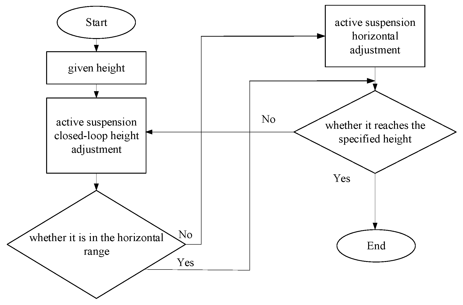
4. Adaptive Active Suspension Height Adjustment

The chassis of the adaptive active suspension is outfitted with ultrasonic displacement sensors positioned at the front and rear axles. These sensors, in conjunction with hydraulic cylinders, facilitate targeted height adjustments. When the active suspension is level, the mean value of both sensors serves as the feedback. In non-horizontal road conditions, when upward adjustment is required, the sensor with the greater measurement value is used for feedback; conversely, for downward adjustments, the sensor with the smaller measurement value is employed.

Leveling must also be considered during the height adjustment process of the active suspension. Due to the uneven load distribution and varying characteristics of hydraulic cylinders, a certain ratio coefficient is applied to each control volume in level road conditions to ensure maximum synchronization of all four hydraulic cylinders. However, under non-horizontal road conditions, the load conditions on each hydraulic cylinder may change, leading to inconsistencies in their actions. Therefore, constant monitoring of the body condition and leveling is necessary throughout the height adjustment process to achieve horizontal ascent or descent of the active suspension. Throughout the height adjustment process, α and β are maintained within the allowable error range to ensure proper leveling.

The height specified by the remote control serves as the target value, while the measured value from the displacement sensor is employed as feedback to construct the height PID closed-loop regulator. Simultaneously, the horizontal attitude of the body must be considered during the ascent or descent process.

After the remote control sends the upward command, the total controller receives the remote-control command and makes the hydraulic cylinder of the wheel legs move upward through four proportional valves. The hydraulic cylinder always detects the body attitude during the rising process, and if the body is in a non-horizontal orientation, it will be adjusted horizontally and then adjusted in height again.

The active suspension height closed-loop process is shown in Figure 15.

After the closed-loop height adjustment, the gyroscope checks whether the body falls within a designated horizontal range. If it does not, leveling is still necessary. The flowchart detailing the algorithm for height adjustment in the adaptive active suspension is presented in Figure 16.

5. Kalman Filter

The gyroscope signal often contains considerable noise, which can lead to significant errors if directly applied in PID calculations. Hence, the acquired data require filtering. Kalman filtering (KF) is a widely used algorithm aimed at optimally estimating system state by observing both input and output data through the system state equation [3]. Kalman filtering can achieve real-time acquisition and prediction without storing historical measurement data to obtain the optimal value at the current moment, which is highly suitable for real-time filtering and processing in MCU computing processors [16,17,18,19,20,21,22].

Assume that the state prediction equation of the system is:

$${\widehat{x}}_k^{-}=A{\widehat{x}}_{k-1}+B{u}_k+{\widehat{w}}_k$$

(1)

where ${\widehat{x}}_k^{-}$ indicates the state estimation value of k moments using k − 1 estimation; ${\widehat{x}}_{k-1}$ indicates the optimal estimation value of k − 1 moments; A and B indicate the state transfer matrix; B indicates the state control matrix, which is a constant in a one-dimensional state; $u_k$ indicates the state control quantity of k moments, and the actual test signals are not controlled by other variables, which is considered to be $u_k$ = 0; and ${\widehat{w}}_k$ is the estimation noise of k moments.

In the system sampling period, the k moment and k − 1 moment values are basically the same; then, the discrete Kalman filter state prediction equation without a control volume is:

$${\widehat{x}}_k^{-}=A{\widehat{x}}_{k-1}$$

(2)

The prediction equation for the covariance is:

$$P_k^{-}=A{P}_{k-1}{A}^T+Q$$

(3)

where $P_k^{-}$ denotes the estimated covariance matrix corresponding to moment k, the corresponding covariance matrix, and Q is the covariance of the system process. The Kalman gain can be calculated by obtaining the system covariance, and the equation for calculating the Kalman gain is:

$${\mathrm{K}}_k=P_k^{-}{H}^T{(H{P}_k^{-}{H}^T+R)}^{-1}$$

(4)

where K_k denotes the Kalman gain at moment k; H is the parameter matrix of the measurement model, and the one-dimensional time-varying variable can be set to 1; and R is the covariance of the noise.

Using the state estimation value at time k and the measurement result at time k, the optimal estimation value at time k, also known as the filtered value at time k, can be derived.

$${\widehat{x}}_k={\widehat{x}}_k^{-}+K_k(z_k-H{\widehat{x}}_k^{-})$$

(5)

where ${\widehat{x}}_k$ denotes the optimal estimate of the state at moment k and $z_k$ is the measured value at moment k. To ensure that the next iteration runs properly, the covariance of ${\widehat{x}}_k$ at moment k needs to be updated:

$$P_k=(I-K_{k}H)P_k^{-}$$

(6)

$P_k$ is the covariance of ${\widehat{x}}_k$ at moment k, and I is the unit matrix, which in the one-dimensional state is the constant value 1. $P_k$ enters the next iteration as $P_k^{-}$ in Equation (5).

6. Active Suspension Ackermann Steering

To ensure smooth maneuvering and prevent sideslip during turns, the active suspension adjusts the deflection angle of the inner and outer tires differently, resulting in a smaller turning radius for the inner tires. With each of the four wheel legs operating independently, software control is necessary to manage the steering angle of the inner and outer tires during turns, following the Ackermann steering principle. Active suspension steering includes two-wheel cornering steering and four-wheel cornering steering. Two-wheel cornering steering includes front-wheel and rear-wheel cornering steering, while four-wheel steering comprises four-wheel same-direction and four-wheel reverse steering. Various active suspension steering configurations are depicted in Figure 17 and Figure 18. The direction of the arrow indicates the turning direction.

Among the four types of steering mentioned above, front-wheel two-wheel steering is the most commonly encountered in daily life, while four-wheel reverse steering exhibits the smallest turning radius during motion. Here, we focus solely on analyzing the distribution relationship of turning angles during front-wheel Ackermann steering and four-wheel reverse Ackermann steering.

6.1. Front-Wheel Ackermann Steering Corner Distribution

Front-Wheel Ackermann Steering Corner Distribution

Figure 19 illustrates the front-wheel Ackermann steering model during cornering with active suspension. This model delineates the correlation among the steering angles of the front inboard and outboard wheels, the body length, the wheelbase, and the turning radius. During the Ackermann steering process, α₁ is the actively given angle and β₁ is the angle calculated based on α_1.

Ackermann steering can be achieved when the front wheels of the suspension chassis are steered when Equation (7) is satisfied by α₁, β₁

$$\cot {\beta }_1-\cot {\alpha }_1=\frac{K}{L}$$

(7)

where α₁ is the inner wheel turning angle of the active suspension, β₁ is the outer wheel turning angle of the active suspension, L is the axle distance between the front and rear axles, K is the spacing between the two wheels, and R is the turning radius. When controlling the front-wheel steering, if the inner-wheel turning angle is α₁₁, then the outer-wheel turning angle β₁₁ is.

$${\beta }_{11}=\mathrm{arccot}(\frac{K}{L}+\cot {\alpha }_1)$$

(8)

6.2. Four-Wheel Reverse-Turn Ackermann Corner Distribution

The four-wheel reverse turning process offers the smallest turning radius, resulting in quicker response times and greater flexibility in active suspension turning. However, higher turning speeds may compromise body stability. As the rotational speed of the active suspension remains moderate during turning, there is a larger stability margin for the body, making the four-wheel reverse turning method suitable. The four-wheel reverse Ackermann steering model during active suspension turning is depicted in Figure 20, outlining the relationship among the four-wheel steering angle, body length, wheelbase, and turning radius.

In Figure 20, δ_fr is the right front wheel Ackermann corner, δ_fl is the left front wheel Ackermann corner, δ_rr is the right rear wheel Ackermann corner, and δ_rl is the left rear wheel Ackermann corner. δ_f sets the corner for the front wheels, and δ_f sets the corner for the rear wheels.

During a left turn, the geometric relationship illustrated in the Figure becomes apparent.

$$\left\{\begin{array}{l}\frac{L_a}{\tan {\delta }_f}=\frac{L_b}{\tan {\delta }_r}\\ L=L_a+L_b\end{array}\right.$$

(9)

where L_a is the distance from the steering instantaneous center of the circle to the front axle and L_b is the distance from the steering instantaneous center of the circle to the rear axle. Transforming Equation (9), the expressions of L_a and L_b are

$$\left\{\begin{array}{l}{L}_a=\frac{L\tan {\delta }_f}{\tan {\delta }_f+\tan {\delta }_r}\\ L_b=\frac{L\tan {\delta }_r}{\tan {\delta }_f+\tan {\delta }_r}\end{array}\right.$$

(10)

According to the geometric relationship in Figure 20, the expressions of δ_fr, δ_fl, δ_rr, and δ_rl during the four-wheel reverse turn are shown in Equation (11):

$$\left\{\begin{array}{l}\cot {\delta }_{fr}=\cot {\delta }_f+\frac{B}{2L_a}\\ \cot {\delta }_{fl}=\cot {\delta }_f-\frac{B}{2L_a}\\ \cot {\delta }_{rr}=\cot {\delta }_r+\frac{B}{2L_b}\\ \cot {\delta }_{rl}=\cot {\delta }_r-\frac{B}{2L_b}\end{array}\right.$$

(11)

By substituting Equation (10) into Equation (11), the Ackermann corner assignments of δ_fr, δ_fl, δ_rr, and δ_rl during a four-wheel reverse turn are given as

$$\left\{\begin{array}{l}\cot {\delta }_{fr}=\arctan (\frac{2L{\tan }^2{\delta }_f}{B{\tan }^2{\delta }_f+B\tan {\delta }_f\tan {\delta }_r+2L\tan {\delta }_f})\\ \cot {\delta }_{fl}=\arctan (\frac{2L{\tan }^2{\delta }_f}{-B{\tan }^2{\delta }_f-B\tan {\delta }_f\tan {\delta }_r+2L\tan {\delta }_f})\\ \cot {\delta }_{rr}=\arctan (\frac{2L{\tan }^2{\delta }_r}{B{\tan }^2{\delta }_r+B\tan {\delta }_f\tan {\delta }_r+2L\tan {\delta }_r})\\ \cot {\delta }_{rl}=\arctan (\frac{2L{\tan }^2{\delta }_r}{-B{\tan }^2{\delta }_r-B\tan {\delta }_f\tan {\delta }_r+2L\tan {\delta }_r})\end{array}\right.$$

(12)

The basic turning angles of the front and rear wheels during the four-wheel reverse turn of the active suspension δ_f = δ_r = δ are set for computational convenience; then, Equation (12) can be simplified as

$$\left\{\begin{array}{l}{\delta }_{fr}={\delta }_{rr}=\arctan (\frac{L\tan \delta }{B\tan \delta +L})\\ {\delta }_{fl}={\delta }_{rl}=\arctan (\frac{L\tan \delta }{-B\tan \delta +L})\end{array}\right.$$

(13)

The Ackermann angle of the four wheels during a four-wheel reverse turn can be calculated by giving the basic torque δ.

7. Analysis of the Experimental Results

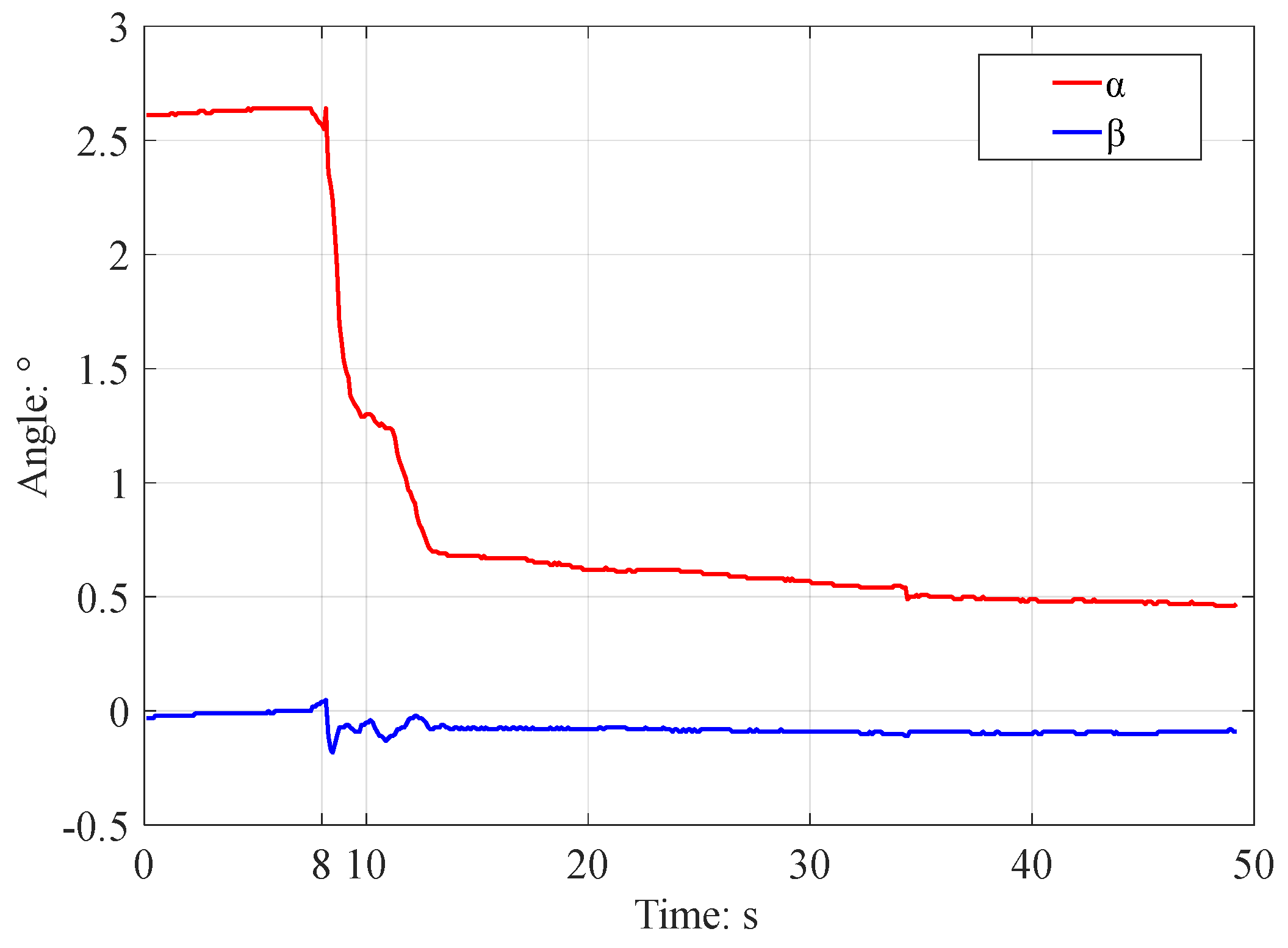
7.1. Analysis of Leveling Results

During the leveling process, there is a tolerance for α and β, allowing for a balance between system accuracy and adjustment time. Setting a smaller error value improves leveling precision but increases adjustment time. To account for accuracy and time, the maximum allowable angular error of α and β is ±0.5°. The maximum allowable angle error of x and y is ±0.5°. The height of the hydraulic cylinder was adjusted manually through the remote control, with options like front high/back low, front low/back high, left high/right low, and left low/right high, as well as specific angle adjustments for each corner. Pressing the “auto-leveling” button triggers the total controller to initiate auto-leveling, recording gyroscope roll angle and pitch angle changes during experiments.

Figure 21 illustrates the angle change curve during automatic leveling after manually adjusting the adaptive active suspension system to a high front-right corner state. Initially, β is close to 0°, while α is around 2.6°. Throughout the leveling process, α gradually decreases while maintaining a relatively stable angle. After automatic leveling, β approaches 0°, with α falling within 0° to 0.5°, meeting the system’s maximum angle deviation and achieving the desired level effect.

Figure 22 shows the angular change curve of automatic leveling after manually adjusting the adaptive active suspension system to the state of the high rear-left corner. The value of β in the initial state is near 0°, and α is approximately −3°. During the leveling process, α gradually increases and the angle of β is basically unchanged. After automatic leveling, β approaches 0°, −0.5° < α < 0°, which meets the maximum angle deviation value of the system and achieves the set leveling effect.

Figure 23 shows the angular change curve of automatic leveling after manually adjusting the adaptive active suspension system to the state of the high front−left corner. The value of β in the initial state is near 0°, and α is 1.2°. During the leveling process, α decreases gradually and the change in the angle of β is not obvious. After automatic leveling, β approaches −0.1°, 0° < α < 0.5°, which meets the maximum angle deviation value of the system and achieves the set leveling effect.

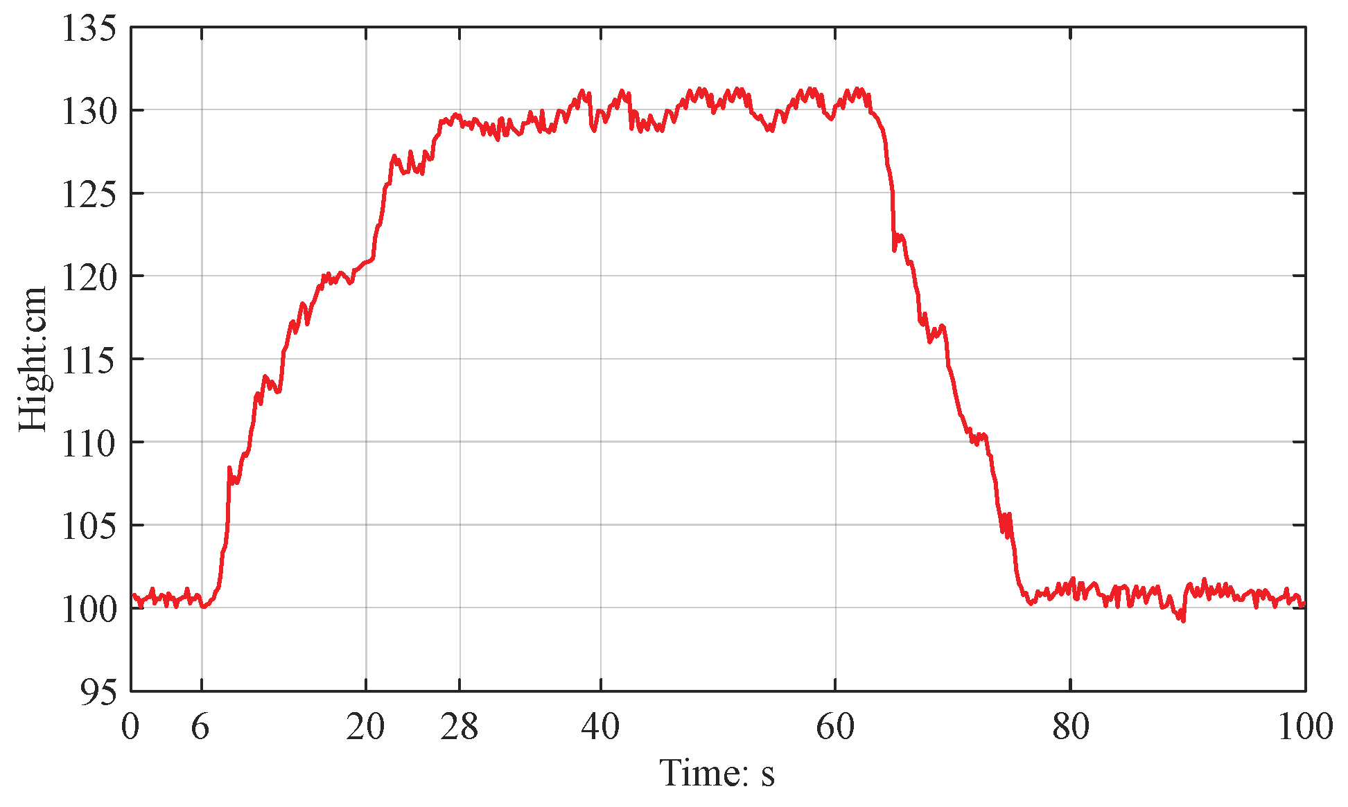
7.2. Analysis of the Upgrading Results

In the process of active suspension height adjustment, the allowable height value has a certain error; the smaller the error value is, the higher the system leveling accuracy, but the longer the system adjustment time. To consider the accuracy of the height adjustment and the leveling time, the allowable error of the height is 5 cm. The body height is set through the remote control during the experiment, and the total controller controls the four wheel leg hydraulic cylinders for the height condition according to the height sensor measurement data. The starting moment for adjusting the body height to 100 cm and the experimental process for recording the height sensor change data are shown in Figure 24.

Based on the experimental results, it is evident that when the body height is set to 130 cm around 6 s, the active suspension smoothly achieves the targeted 130 cm position with the assistance of the wheel-leg hydraulic cylinder. The error upon reaching the target position is under 5 cm. Similarly, when the body height is set to 100 cm around 60 s, the active suspension stabilizes at 100 cm by approximately 80 s through closed-loop height adjustment, with the body height error also remaining under 5 cm.

8. Conclusions

A special vehicle’s adaptive active suspension control system is constructed using components like wheel-hub motors, hydraulic cylinders, gyroscopes, height sensors, STM32F4 controllers, etc. This system facilitates adaptive active suspension actions such as forward, reverse, diagonal, traverse, height adjustment, leveling, and Ackermann turn signals at varying speeds. Through the hydraulic cylinder control system, an automatic leveling and height adjustment control strategy for adaptive active suspension vehicles is proposed, ensuring swift leveling and height adjustments within a certain range. After several experiments, we have obtained some preliminary results. Irrespective of the vehicle body’s different attitudes and heights, the leveling control strategy outlined in this paper reliably achieves the set horizontal attitude and specified height. By employing the Ackermann steering principle via software control, both front-wheel steering and four-wheel reverse steering systems of the special vehicle are enhanced, thereby improving its cornering capability. This control strategy for adaptive active suspension systems serves as a valuable reference for the design and control of other special vehicles.

References

1. Fitzsimmons, J.A. A methodology for emergency ambulance deployment. Manag. Sci. 1973, 19, 627–636. [Google Scholar] [CrossRef]
2. Kim, D.; Jeong, D.; Seo, Y. Intelligent design for simulation models of weapon systems using a mathematical structure and case-based reasoning. Appl. Sci. 2020, 10, 7642. [Google Scholar] [CrossRef]
3. Bélanger, V.; Ruiz, A.; Soriano, P. Recent optimization models and trends in location, relocation, and dispatching of emergency medical vehicles. Eur. J. Oper. Res. 2019, 272, 1–23. [Google Scholar] [CrossRef]
4. Li, M.; Imou, K.; Wakabayashi, K.; Yokoyama, S. Review of research on agricultural vehicle autonomous guidance. Int. J. Agric. Biol. Eng. 2009, 2, 1–16. [Google Scholar]
5. Liu, Y.; Wu, J.; Tang, J.; Wang, W.; Wang, X. Scheduling optimisation of multi-type special vehicles in an airport. Transp. B Transp. Dyn. 2022, 10, 954–970. [Google Scholar] [CrossRef]
6. Wang, Y.; Yu, J.; Yan, B.; Wang, G.; Shan, Z. BSV-PAGS: Blockchain-based special vehicles priority access guarantee scheme. Comput. Commun. 2020, 161, 28–40. [Google Scholar] [CrossRef]
7. Liu, H.; Li, S. Speed control for PMSM servo system using predictive functional control and extended state observer. IEEE Trans. Ind. Electron. 2011, 59, 1171–1183. [Google Scholar] [CrossRef]
8. Vo, H.H. Sliding mode speed controller design for field oriented controlled PMSM drive of an electric vehicle. J. Adv. Eng. Comput. 2023, 7, 164–173. [Google Scholar] [CrossRef]
9. Keshari, R.; Jarariya, S. Performance Analysis of PMSM-Electric Vehicle with Fuzzy Logic Controller. Int. J. Progress. Res. Eng. Manag. Sci. 2023, 3, 562–570. [Google Scholar]
10. Jian, L. Research status and development prospect of electric vehicles based on hub motor. In Proceedings of the 2018 China International Conference on Electricity Distribution (CICED), Tianjin, China, 17–19 September 2018. [Google Scholar]
11. Shi, Z.; Sun, X.; Cai, Y.; Yang, Z. Robust design optimization of a five-phase PM hub motor for fault-tolerant operation based on Taguchi method. IEEE Trans. Energy Convers. 2020, 35, 2036–2044. [Google Scholar] [CrossRef]
12. Msaddek, H.; Mansouri, A.; Brisset, S.; Trabelsi, H. Design and optimization of PMSM with outer rotor for electric vehicle. In Proceedings of the 2015 IEEE 12th International Multi-Conference on Systems, Signals & Devices (SSD15), Mahdia, Tunisia, 16–19 March 2015. [Google Scholar]
13. Dai, Y.; Song, L.; Cui, S. Development of PMSM drives for hybrid electric car applications. IEEE Trans. Magn. 2006, 43, 434–437. [Google Scholar] [CrossRef]
14. Kim, H.; Son, J.; Lee, J. A high-speed sliding-mode observer for the sensorless speed control of a PMSM. IEEE Trans. Ind. Electron. 2010, 58, 4069–4077. [Google Scholar] [CrossRef]
15. Said-Romdhane, M.B.; Skander-Mustapha, S.; Belhassen, R. Adaptive Deadbeat Predic-tive Control for PMSM-based solar-powered electric vehicles with enhanced stator resistance compensation. Sci. Technol. Energy Transit. 2023, 78, 35. [Google Scholar] [CrossRef]
16. Khodarahmi, M.; Maihami, V. A review on Kalman filter models. Arch. Comput. Methods Eng. 2023, 30, 727–747. [Google Scholar] [CrossRef]
17. Feng, S.; Li, X.; Zhang, S.; Jian, Z.; Duan, H.; Wang, Z. A review: State estimation based on hybrid models of Kalman filter and neural network. Syst. Sci. Control. Eng. 2023, 11, 2173682. [Google Scholar] [CrossRef]
18. Bai, G.; Su, Y.; Rahman, M.M.; Wang, Z. Prognostics of Lithium-Ion batteries using knowledge-constrained machine learning and Kalman filtering. Reliab. Eng. Syst. Saf. 2023, 231, 108944. [Google Scholar] [CrossRef]
19. Naya, M.Á.; Sanjurjo, E.; Rodríguez, A.J.; Cuadrado, J. Kalman filters based on multibody models: Linking simulation and real world. A comprehensive review. Multibody Syst. Dyn. 2023, 58, 479–521. [Google Scholar] [CrossRef]
20. Feng, Z.; Wang, G.; Peng, B.; He, J.; Zhang, K. Distributed minimum error entropy Kalman filter. Inf. Fusion 2023, 91, 556–565. [Google Scholar] [CrossRef]
21. Valade, A.; Acco, P.; Grabolosa, P.; Fourniols, J.-Y. A study about Kalman filters applied to embedded sensors. Sensors 2017, 17, 2810. [Google Scholar] [CrossRef] [PubMed]
22. Budak, S.; Tekïn, M.H.; Durdu, A.; Sungur, C. Kalman Filter and PID Application on Underwater Vehicles. Turk. J. Forecast. 2022, 6, 27–33. [Google Scholar] [CrossRef]
Figure 1. Adaptive active suspension system structure.
Processes 12 01483 g001
Figure 2. Three-dimensional diagram of adaptive active suspension.
Processes 12 01483 g002
Figure 3. Shrinkage control of a single hydraulic cylinder.
Processes 12 01483 g003
Figure 4. Several unbalanced-attitude adjustment processes.
Processes 12 01483 g004
Figure 5. Schematic diagram of automatic leveling control.
Processes 12 01483 g005
Figure 6. Schematic diagram of front high/rear low leveling control.
Processes 12 01483 g006
Figure 7. Schematic diagram of front low/rear high leveling control.
Processes 12 01483 g007
Figure 8. Schematic diagram of left high/right low leveling control.
Processes 12 01483 g008
Figure 9. Schematic diagram of left low/right high leveling control.
Processes 12 01483 g009
Figure 10. Schematic diagram of front right corner high leveling control.
Processes 12 01483 g010
Figure 11. Schematic diagram of front left corner high leveling control.
Processes 12 01483 g011
Figure 12. Schematic diagram of rear right corner high leveling control.
Processes 12 01483 g012
Figure 13. Schematic diagram of rear-left corner height leveling control.
Processes 12 01483 g013
Figure 14. Flowchart of the adaptive active suspension leveling.
Processes 12 01483 g014
Figure 15. Hydraulic cylinder height adjustment.
Processes 12 01483 g015
Figure 16. Adaptive active suspension height adjustment flowchart.
Processes 12 01483 g016
Figure 17. Schematic diagram of active suspension front- and rear-wheel steering.
Processes 12 01483 g017
Figure 18. Schematic diagram of active suspension with four wheels steering in the same direction and in the opposite direction.
Processes 12 01483 g018
Figure 19. Ackermann steering model for the front wheels of the active suspension system.
Processes 12 01483 g019
Figure 20. Ackermann steering model for four-wheel reverse cornering with active suspension.
Processes 12 01483 g020
Figure 21. Angle data curve of automatic leveling in the high front−right corner state.
Processes 12 01483 g021
Figure 22. Angle data curve of auto−leveling for the high back−left corner state.
Processes 12 01483 g022
Figure 23. Angle data curve of auto−leveling for the high front−left corner state.
Processes 12 01483 g023
Figure 24. Angle data curve for automatic body height leveling.
Processes 12 01483 g024