Double-Closed-Loop Model Predictive Control Based on a Linear Induction Motor

Abstract

The conventional PI control, which has been extensively employed in the high-performance control of linear induction motors, has the benefit of a straightforward concept, quick dynamic response, and simple control. Nevertheless, the linear induction motor is more susceptible to outside disturbances and mismatched parameters since it is a highly linked, high-order, nonlinear, time-varying, complex system. Because of this, this paper proposes a double-closed-loop control of the linear induction motor, whose speed and current loops are the model-predictive speed controller and the model-predictive current controller, respectively, to solve the problems of speed overshoot and oscillation when the linear induction motor is operated under PI control. The findings demonstrate the benefits of the suggested control strategy, which significantly enhances the linear induction motor’s speed control performance. These benefits include improved dynamic performance, limited overshooting, and robust resistance to load disturbance.

1. Introduction

Model predictive control (MPC) has been used more and more in the fields of power electronics and motor control in recent years as the computational capacity from different chips has increased. A variety of high-performance devices, including FPGA, ARM, and DSP, have been very helpful in the creation of MPC. By listing all of the inverter’s switching states, MPC chooses the one with the smallest value function as the best controller output. This process is based on the dynamic mathematical model of the motor and takes into account the inverter’s discrete features [1,2,3]. Its benefits include a straightforward principle, quick transient reaction, a very flexible cost function, the ease of handling nonlinear restrictions, and the ability to have many control variables or targets [4,5,6].

Given that the linear induction motor (LIM) is a complicated, multivariable, nonlinear, highly linked, variable parameter object, the performance of the motor in complex working conditions is not limited by its application occasions when using a traditional PID control, despite the fact that it can meet a certain range of control requirements. This is because it depends on an accurate model of the LIM, is highly susceptible to external perturbations and parameter mismatch, and is difficult to obtain satisfactory speed regulations and positioning performance [7,8].

The range of applications for LIM servo systems is growing, and with it, so are the low- and medium-speed performance requirements of modern servo systems. Examples of these applications include wave energy power generation, CNC machine tools, urban rail transit, electromagnetic catapults, aerospace, and other fields. These applications demand good characteristics and anti-jamming performance—that is, the ability of the motor to run smoothly under specific load and speed changes while responding swiftly to changes in the commanded value. To control the motor, the MPC takes a multi-step technique. MPC has many benefits, including a good control effect, high accuracy, strong robustness, and low requirements for model accuracy. Its application in LIM servo systems is highly promising because it uses control strategies like multi-step prediction, feedback correction, and rolling optimization.

Finite control set model predictive current control (FCS-MPCC), finite control set model predictive torque control (FCS-MPTC), finite control set model predictive chain control (FCS-MPFC), and finite control set model predictive speed control (FCS-MPSC) are the four general categories into which finite control set model predictive current control (FCS-MPC) can be divided based on the control objective. The cost function primarily represents their differences: in FCS-MPCC, the control objective is current, and the evaluation index is current error; in FCS-MPTC, the control objective is torque, and the evaluation index is torque error; in FCS-MPFC, the control objective is magnetic chain, and the evaluation index is magnetic chain error; and in FCS-MPSC, the control objective is speed, and the evaluation index is speed error. In order to solve the problems of large overshoot and poor disturbance resistance under PI control, fast response speeds, little steady-state error, and nearly no overshoot are among the benefits of the fully predictive cascade speed and current control approach presented in [9] with model predictive control for both the speed outer loop and the current inner loop. In [10], a linear controller that suppresses the high-frequency current component and removes the steady-state error is included in a short prediction time domain predictive speed control approach that aims to achieve a quick reaction from the control system. Using the second-order Taylor series model of the quadratic cost function, the model predictive direct speed control (MPSC) approach proposed in [11] is based on the Taylor series model and derives the fundamental voltage vectors with the same control period, improving the motor’s dynamic and static control performance. Using a reference voltage vector to construct a cost function, the weighting factor selection problem is resolved in [12] by proposing a predictive direct speed control method without weighting factors. Additionally, an extended sliding mode load torque observer was designed to increase the motor’s robustness.

Furthermore, in order to improve the speed and current regulation performance under PI control, ref [13] suggests using a model predictive current control technique that eliminates the nonlinear coupling of the d- and q-axis currents in surface-mounted permanent magnet synchronous motors using the control rate to feedforward and feedback control the current. In undertaking this, the decoupling effect is enhanced, and its dynamic performance is also enhanced. In [14], a speed prediction current decoupling control for permanent magnet synchronous motors is proposed. This control improves the dynamic response performance of the control system by introducing model predictive control into the speed loop control and making use of its rolling optimization and feedback correction characteristics.

While the traditional FCS-MPSC removes the double-closed-loop structure by combining the speed and current in the cost function, it still has two major urgent issues with its single-loop structure that impede the motor’s dynamic response performance. First, there is a greater current and torque pulsation because the motor’s electrical time constant is smaller than its mechanical time constant, causing the current to fluctuate considerably faster than the speed. Second, the control period for both the speed and current must be the same since they are both contained in the cost function; nevertheless, in high-frequency speed measurements, the encoder produces some inaccuracies.

This means that even while the double-closed-loop structure of the traditional FCS-MPSC has worse dynamic performance than the single-loop structure, there are still some issues. Additionally, keep in mind that PI controllers—which are less resistant to changes in motor parameters because they are harder to update and have fixed values for PI parameters—are used for the majority of speed loop controls in the double closed-loop structure.

Thus, a double-closed-loop model-predictive control method is proposed for LIM in this paper to achieve the smooth control of LIM speed and prevent the issue of its speed being prone to overshooting and oscillation under PI control. This method constitutes a structure combining MPSC and the model predictive current control (MPCC), which improves the dynamic and disturbance-resistant performance of the motor and is nearly free of overshooting.

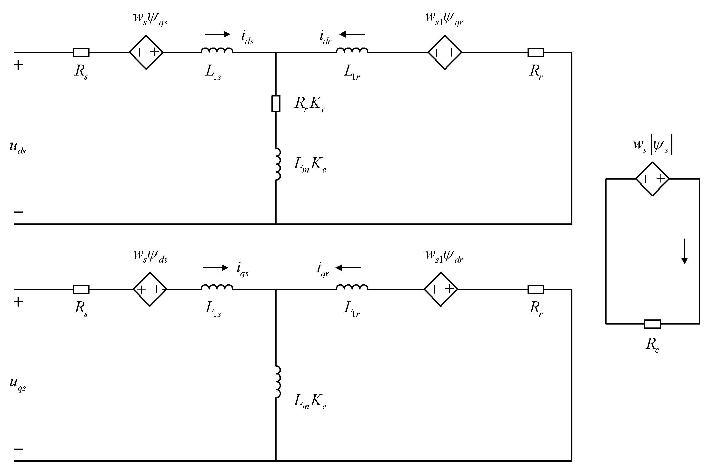
2. Mathematical Modeling of Linear Induction Motors

Generally speaking, after correcting the pertinent motor parameters and taking into account the impact of dynamic side-end effects, the LIM equivalent circuit is derived from the traditional rotary induction motor equivalent circuit. The iron consumption brought on by the primary stage’s leakage inductance, however, cannot be disregarded in the computation of motor losses due to the linear induction motor’s huge air gap and primary leakage inductance. In addition, the iron consumption branch current is significantly lower than the extraction branch current, which can be independent of the iron consumption branch, and the secondary loss is much smaller than the primary loss, meaning that the secondary leakage inductance is frequently disregarded in the mathematical model. In light of this, the paper uses the dq-axis asymmetric equivalent circuit of an LIM with an independent iron dissipation branch, as seen in Figure 1.

This is equivalent to shunting the excitation inductance by connecting an inductor in parallel with the LIM excitation circuit. The model starts with the Q coefficient of the Duncan model, and the secondary guide plate eddy current generates a magnetic field that partially offsets the motor air gap magnetic field. K_e and K_r, which are the excitation inductance attenuation coefficient and secondary eddy current loss coefficient, respectively, are derived in this manner; the specific expressions are provided in the Appendix for Equations (A1)–(A3).

Consequently, the following is an appropriate way to write the asymmetric equivalent circuit voltage and flux equations of the LIM:

$$\{\begin{array}{l}{u}_{\mathrm{ds}}=i_{\mathrm{ds}}{R}_{\mathrm{s}}+p{\psi }_{\mathrm{ds}}-{\omega }_{\mathrm{s}}{\psi }_{\mathrm{qs}}+(i_{\mathrm{ds}}+i_{\mathrm{dr}})R_{\mathrm{r}}{K}_r\\ u_{\mathrm{qs}}=i_{\mathrm{qs}}{R}_{\mathrm{s}}+p{\psi }_{\mathrm{qs}}+{\omega }_{\mathrm{s}}{\psi }_{\mathrm{ds}}\\ 0=i_{\mathrm{dr}}{R}_{\mathrm{r}}+p{\psi }_{\mathrm{dr}}-{\omega }_{\mathrm{sl}}{\psi }_{\mathrm{qr}}+(i_{\mathrm{ds}}+i_{\mathrm{dr}})R_{\mathrm{r}}{K}_r\\ 0=i_{\mathrm{qr}}{R}_{\mathrm{r}}+p{\psi }_{\mathrm{qr}}+{\omega }_{\mathrm{sl}}{\psi }_{\mathrm{dr}}\end{array}$$

(1)

$$\{\begin{array}{l}{\psi }_{\mathrm{ds}}=L_{\mathrm{ls}}{i}_{\mathrm{ds}}+L_{\mathrm{m}}{K}_e(i_{\mathrm{ds}}+i_{\mathrm{dr}})\\ {\psi }_{\mathrm{qs}}=L_{\mathrm{ls}}{i}_{\mathrm{qs}}+L_{\mathrm{m}}{K}_e(i_{\mathrm{qs}}+i_{\mathrm{qr}})\\ {\psi }_{\mathrm{dr}}=L_{\mathrm{lr}}{i}_{\mathrm{dr}}+L_{\mathrm{m}}{K}_e(i_{\mathrm{ds}}+i_{\mathrm{dr}})\\ {\psi }_{\mathrm{qr}}=L_{\mathrm{lr}}{i}_{\mathrm{qr}}+L_{\mathrm{m}}{K}_e(i_{\mathrm{qs}}+i_{\mathrm{qr}})\end{array}$$

(2)

The thrust equation based on secondary flux orientation can be written as follows:

$$F=\beta L_{\mathrm{m}\mathrm{e}}(i_{\mathrm{dr}}{i}_{\mathrm{qs}}-i_{\mathrm{qr}}{i}_{\mathrm{ds}})=\beta {\displaystyle \frac{L_{\mathrm{m}\mathrm{e}}}{L_{\mathrm{m}\mathrm{e}}+L_{\mathrm{lr}}}}{\psi }_{\mathrm{dr}}{i}_{\mathrm{qs}}$$

(3)

where p is the differential operator, β = π/τ. To simplify the expression below, let L_me = L_mK_e, R_re = R_rK_r.

The mechanical equations of motion are as follows:

$$F-F_l=m{\displaystyle \frac{dv}{dt}}+Bv$$

(4)

where F, F_l, B, and m are the electromagnetic thrust, load, system viscosity coefficient, and traction weight of the linear induction motor, respectively.

3. Dual-Closed-Loop Model Predictive Control

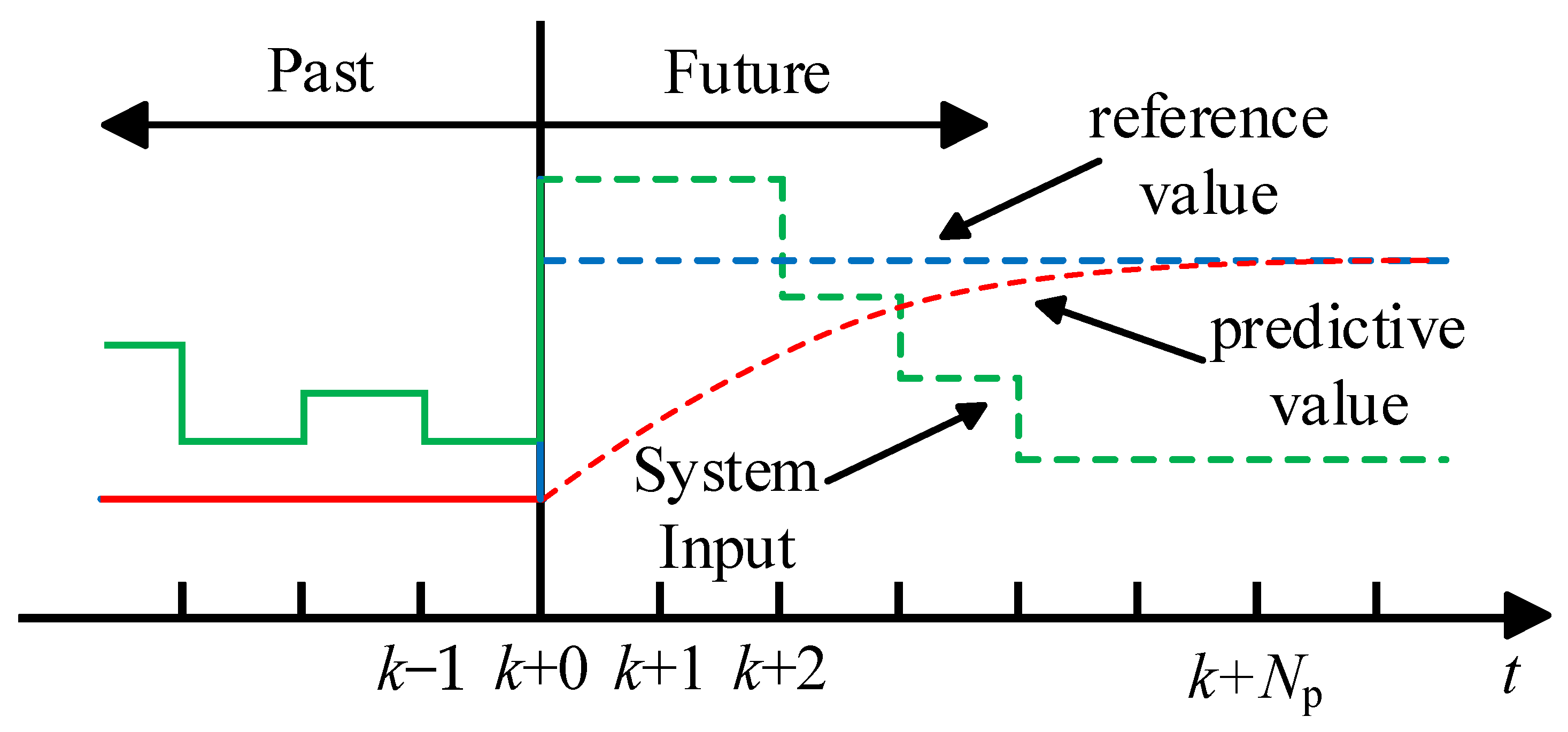
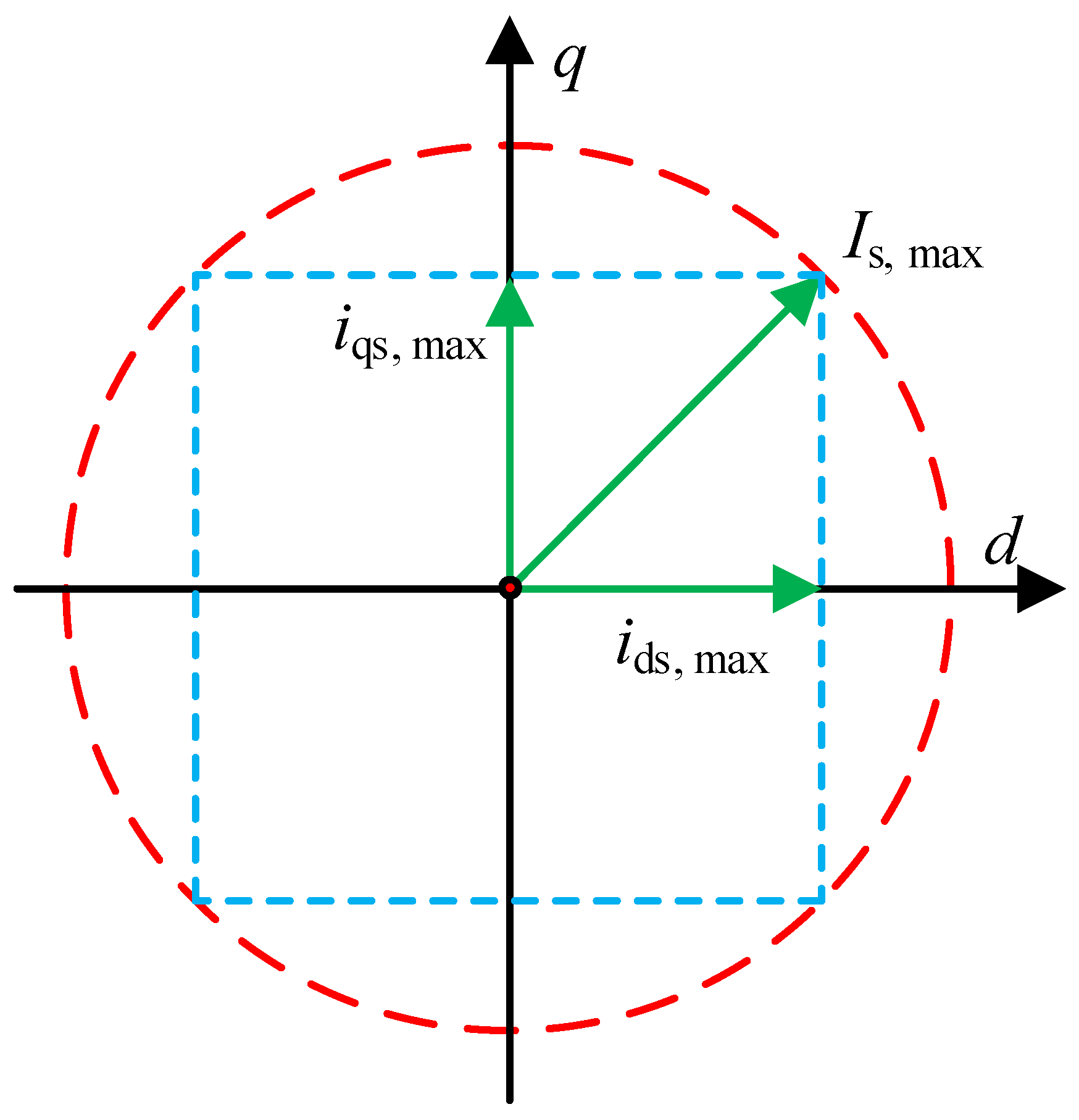
3.1. Model Predictive Current Control

MPC is the best kind of control. The process is illustrated in Figure 2 and involves using the mathematical model of the motor and the state variables measured prior to the kth moment to predict the future value of the system’s state within a predetermined time period k + N. Next, the optimal input signal that brings the predicted value as close to the reference value as possible is selected by evaluating the cost function set in advance in accordance with one’s own control needs. Finally, the corresponding switching signal is used to control the inverter to realize the tracking of the reference value.

The control method is a control strategy that is based on the mathematical model of the control object. First, in order to solve the optimal control quantity, which is then applied to the controlled object to accurately follow the reference trajectory, the cost function is set in accordance with the control requirements. Lastly, the prediction time domain is shifted forward by one cycle, and the above steps are repeated to scroll forward.

The three components of MPC control systems are, in summary, the rolling optimization, feedback correction, and prediction model. Figure 3 displays a basic construction block diagram.

(1)

Prediction model

MPC is a control approach that relies on mathematical models; therefore, it is required to choose beforehand which mathematical model best fits the controlled object’s dynamic behavior and can anticipate the controlled object’s behavior in the future time domain. The majority of the state equation is currently utilized as the mathematical model, and its expression is as follows:

$$\{\begin{array}{c}x(k)=Ax(k-1)+Bu(k-1)\\ y(k)=Cx(k)\end{array}$$

(5)

where A is the state coefficient matrix, B is the input coefficient matrix, C is the output coefficient matrix, and x is the controlled object state variable.

The control object’s expected output expression at the sampling moment of (k + l)T_s is displayed as follows using Equation (5):

$$\widehat{y}(k+l)=C\widehat{x}(k+l)=C\left[A^{l}x(k)+{\displaystyle \sum _{i=1}^l{A}^{i-1}Bu(k+l-i)}\right]$$

(6)

(2)

Rolling optimization

Rolling optimization is the process by which the controller repeatedly finds the best answer throughout a fixed number of sampling moments using a performance metric function that is provided. The rolling optimization and the traditional optimal control differ primarily in two ways: first, the rolling optimization computes on-the-go, whereas the traditional optimal control computes off-line; second, the rolling optimization finds the optimal solution in the local time domain, whereas the traditional optimal control solves the whole domain optimal solution.

(3)

Feedback correction

To improve the predictive control of anti-perturbation, feedback correction is achieved via the rolling optimization of the control object’s output value and its actual output value for continuous correction. This allows the actual output value to follow a specified, smooth curve to reach a given value. Additionally, the algorithm continuously updates the parameter mismatches, external perturbations, and other uncertainties resulting from its impact. The predicted value at point A at moment k + 1 is the result of rolling optimization at moment k, as illustrated in Figure 4, but the actual value on the system is at point B. This process determines the ideal voltage vector for the subsequent instant. To prevent the accumulation of prediction errors in the control system, corrected prediction trajectory 2 must be derived by offsetting both the instant k + 1 and prediction trajectory 1 downward. This corrects the prediction error at that particular time.

Equations (1) and (2) allow for the derivation and discretization of the full-order equation of state of the linear induction motor in the dq synchronous rotating coordinate system using the first-order Eulerian discretization method:

$$Y(k)=\left[\begin{array}{cccc}1& 0& 0& 0\\ 0& 1& 0& 0\end{array}\right]\left[\begin{array}{c}{i}_{ds}(k)\\ i_{qs}(k)\\ {\psi }_{dr}(k)\\ {\psi }_{qr}(k)\end{array}\right]$$

(7)

$$\begin{array}{l}\left[\begin{array}{c}{i}_{ds}(k+1)\\ i_{qs}(k+1)\\ {\psi }_{dr}(k+1)\\ {\psi }_{qr}(k+1)\end{array}\right]=\left[\begin{array}{cccc}1-\left[{\displaystyle \frac{1}{{\tau }_{\sigma }^{\prime }}}+{\displaystyle \frac{R_{re}}{\epsilon }}\left(k_r-1\right)\right]T_s& w_s{T}_s& {\displaystyle \frac{T_s}{\epsilon T_r}}+{\displaystyle \frac{R_{re}}{\epsilon }}\left(k_r-1\right)T_s& {\displaystyle \frac{w_r}{\epsilon }}{T}_s\\ -w_s{T}_s& 1-{\displaystyle \frac{T_s}{{\tau }_{\sigma }^{\prime }}}& -{\displaystyle \frac{w_r}{\epsilon }}{T}_s& {\displaystyle \frac{T_s}{\epsilon T_r}}\\ \left[{\displaystyle \frac{L_{me}}{T_r}}+R_{re}\left(k_r-1\right)\right]T_s& 0& 1-\left({\displaystyle \frac{1}{T_r}}+{\displaystyle \frac{R_{re}}{L_r}}\right)T_s& w_{s1}{T}_s\\ 0& {\displaystyle \frac{L_{me}}{T_r}}{T}_s& -w_{s1}{T}_s& 1-{\displaystyle \frac{T_s}{T_r}}\end{array}\right]\left[\begin{array}{c}{i}_{ds}(k)\\ i_{qs}(k)\\ {\psi }_{dr}(k)\\ {\psi }_{qr}(k)\end{array}\right]\\ +\left[\begin{array}{cc}{\displaystyle \frac{T_s}{\sigma L_s}}& 0\\ 0& {\displaystyle \frac{T_s}{\sigma L_s}}\\ 0& 0\\ 0& 0\end{array}\right]\left[\begin{array}{c}{u}_{ds}(k)\\ u_{qs}(k)\end{array}\right]\end{array}$$

(8)

where T_s is the discretized sampling period of the controller, T_r is the secondary time constant, T_r = L_r/R_r, $\epsilon ={\displaystyle \frac{\sigma L_s{L}_r}{L_{me}}}$, $R_{\sigma }=R_s+k_r^2{R}_r={\displaystyle \frac{R_r{L}_{me}^2+R_s{L}_r^2}{L_r^2}}$ is the equivalent resistance, $k_r={\displaystyle \frac{L_m}{L_r}}$ is the secondary coupling factor, ${\tau }_{\sigma }^{\prime }={\displaystyle \frac{\sigma L_s}{R_{\sigma }}}={\displaystyle \frac{\sigma L_s{L}_r^2}{R_r{L}_{me}^2+R_s{L}_r^2}}$ is the instantaneous time constant, ${\tau }_r^{\prime }={\displaystyle \frac{\sigma L_s}{R_r}}$ is the secondary instantaneous time constant, and ${\tau }_s^{\prime }={\displaystyle \frac{\sigma L_s}{R_s}}$ is the primary instantaneous time constant. The subscripts k and k + 1 represent the values of the state variables at the moments k and k + 1, respectively.

Many digital delays introduced during the operation of the control system, such as current sampling, duty cycle updating, deadband, and inverter output, must be taken into account in order to meet the real application. Furthermore, the present limitations are taken into account, and the subsequent cost function is chosen for this paper:

$$g={\left(i_{ds}^{\ast }-i_{ds}(k+2)\right)}^2+{\left(i_{qs}^{\ast }-i_{qs}(k+2)\right)}^2+f(i)$$

(9)

where f(i) is the overcurrent penalty term with the following expression:

$$f(i)=\{\begin{array}{cc}\infty & \sqrt{i_{ds}^2(k+2)+i_{qs}^2(k+2)}>I_{\max }\\ 0& \sqrt{i_{ds}^2(k+2)+i_{qs}^2(k+2)}<I_{\max }\end{array}$$

(10)

wher: I_max is the maximum current limit value, as shown in Figure 5.

3.2. Model Predictive Speed Control

Traditional vector control systems for common linear induction motors include three PI control loops: one for speed control, one for q-axis current control, and one for d-axis current control. The former is used to regulate the motor’s speed, while the latter two are used to regulate its current. PI control offers a wide range of application scenarios because of its advantages, which include its simple structure, ease of operation, and stability in real-world applications.

The application of linear induction motors results from the control method’s inability to simultaneously meet the requirements of fast response and high steady-state accuracy. This is because the linear induction motor control system with edge effect and primary disconnection requires a better speed tracking ability and current responsability. In addition, traditional PI control in PI parameter adjustment is difficult, fixed, and parameter-mismatched when the robustness of the shortcomings of poor parameter adjustment is observed. Consequently, there are very few applications for linear induction motors. In order to effectively improve the control performance of linear induction motors, this work offers a double-closed-loop model predictive control that has a greater control effect than the typical PI control. Equations (3) and (4) allow the following to be deduced:

$${\displaystyle \frac{dv}{dt}}={\displaystyle \frac{1}{m}}(k_T{i}_{qs}-F_l-Bv)$$

(11)

The aforementioned equation can be derived to a second-order derivative as follows:

$${\displaystyle \frac{d^{2}v}{dt}}={\displaystyle \frac{1}{m}}(k_T{\displaystyle \frac{d{i}_{qs}}{dt}}-{\displaystyle \frac{d{F}_l}{dt}}-B{\displaystyle \frac{dv}{dt}})$$

(12)

Using Taylor’s formula to expand and discretize the aforementioned equation results, the following is obtained:

$$v_{k+1}=v_k+T_s·{\dot{v}|}_k+{\displaystyle \frac{T_s^2}{2}}·{\ddot{v}|}_k$$

(13)

where T_s is the velocity loop’s sampling time.

Using Equation (3), Equations (1) and (2) can be obtained:

$$v_{k+1}=v_k+T_{su}·{\left[{\displaystyle \frac{1}{m}}(k_T{i}_{qs}-F_l-Bv)\right]|}_k+{\displaystyle \frac{T_{su}^2}{2}}·{\left[{\displaystyle \frac{1}{m}}(k_T{\displaystyle \frac{d{i}_{qs}}{dt}}-{\displaystyle \frac{d{F}_l}{dt}}-B{\displaystyle \frac{dv}{dt}})\right]|}_k$$

(14)

The preceding equation’s first-order derivative of the major cross-axis current is discretized using forward Eulerian methods.

$${\displaystyle \frac{d{i}_{qs}}{dt}}={\displaystyle \frac{i_{qs}^{k+1}-i_{qs}^k}{T_s}}$$

(15)

Additionally, $i_{qs}^{k+1}=i_{qs}^{\ast }$, $v_{k+1}=v^{\ast }$, and Equation (15) are introduced into Equation (14), where $v^{\ast }$ and $i_{qs}^{\ast }$ are the given values of the linear velocity and primary cross-axis current of the linear induction motor, respectively. This equation can then be solved for a given primary cross-axis current. This is because the load thrust is nearly unchanged during the sampling time.

$$i_{qs}^{\ast }={\displaystyle \frac{-1}{T_s{K}_{T}m}}\left[\begin{array}{l}2m^2(v_k-v^{\ast })+T_s^2{B}^{2}v+T_s^{2}B{F}_l-2mB{T}_{s}v\\ -2m{T}_s{F}_l+m{T}_s{K}_T{i}_{qs}(k)-T_s^2{K}_{T}B{i}_{qs}(k)\end{array}\right]$$

(16)

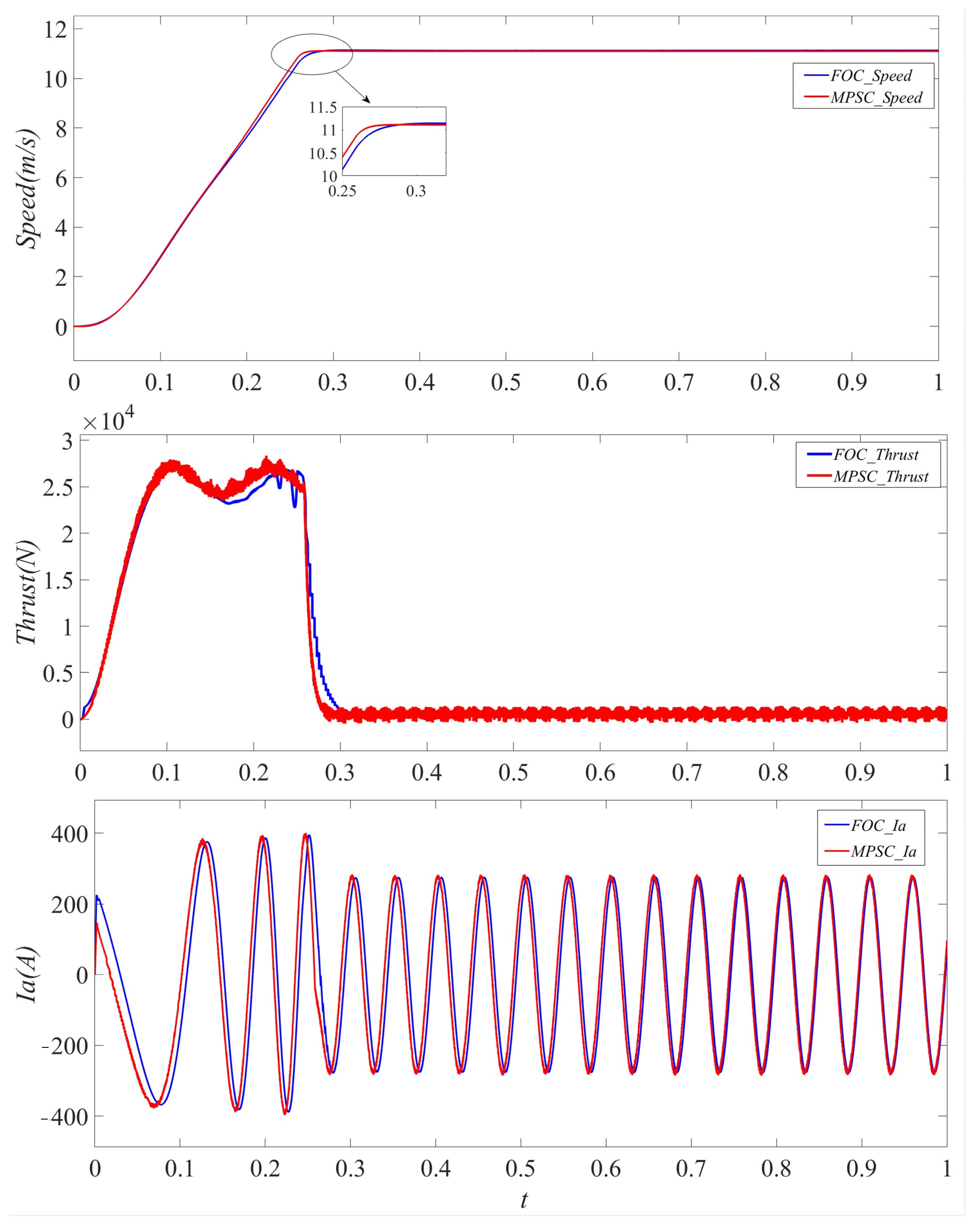
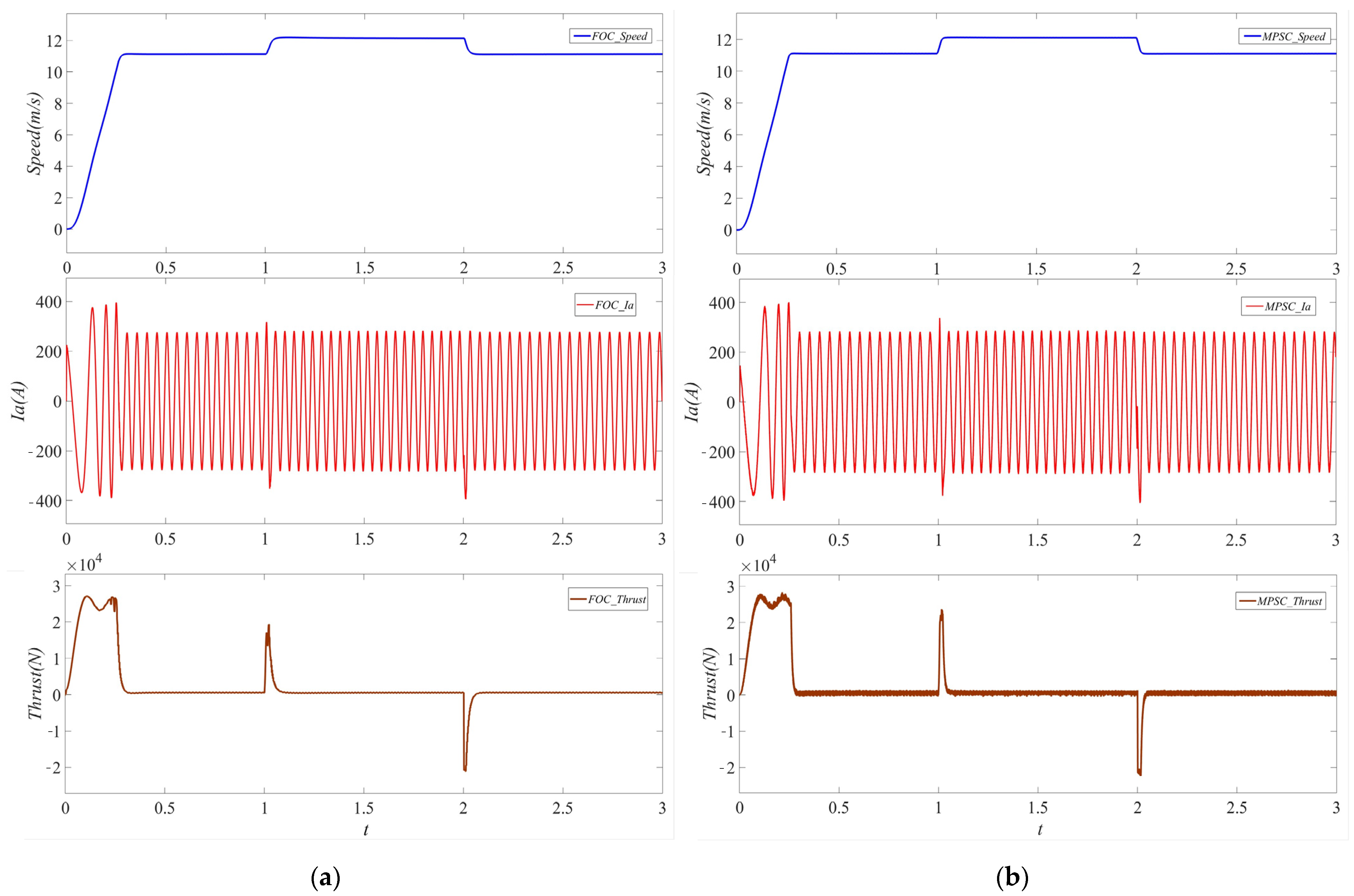
4. Simulation and Analysis

The research object of this paper is a three-phase linear induction motor, the main parameters of which are shown in

Table A1. LIM main parameters.

Parameters	Values	Unit
Pole-pair number	6	-
Pole pitch	0.2808	m
Rated flux	6	Wb
Primary resistance	0.138	Ω
Secondary resistance	46.4	Ω
Iron loss resistance	167	Ω
Magnetizing inductance	0.026477	H
Primary leakage inductance	0.006688	H
Secondary leakage inductance	0.002091	H
Secondary length	2.476	m

of the Appendix. The block diagram for the dual-closed-loop model predictive control system simulation of a linear induction motor is displayed in Figure 6.

The simulated waveforms of the motor’s thrust, speed, and three-phase current under PI and MPSC + MPCC regulation at light-load starting are displayed in Figure 7. The speed and load were set to 11.1 m/s and 600 N, respectively. The control approach suggested in this study has a faster speed response and nearly no overshoot when compared to the PI control, as demonstrated by the simulated waveforms.

The motor is configured, as seen in Figure 8, to abruptly accelerate to 12.1 m/s at 1 s and reduce to 11.1 m/s at 2 s. The simulated waveforms of thrust, A-phase current, and speed show that the MPSC + MPCC performs better at regulating speeds than the PI control.

The motor’s speed, thrust, and A-phase current response waveforms under the PI and MPSC + MPCC control when adding and removing the load are displayed in Figure 9. The motor is programmed to increase the load to 5000 N in one second and decrease the load to 600 N in two seconds. The simulated waveforms clearly show that when adding or removing the load, MPSC + MPCC has superior anti-interference performance with reduced speed variation.

Table 1. Speed response times of the two control strategies under different operating conditions.

	ts(s)
	Constant Speed	Acceleration	Deceleration	Adding Loads	Subtracting Loads
PI	0.259	1.0455	2.0375	1.3195	2.3846
MPSC + MPCC	0.0254	1.0393	2.0346	1.2998	2.3144

and

Table 2. Speed fluctuation of the two control strategies under different operating conditions.

	ts(s)
	Adding Loads	Subtracting Loads
PI	0.1001	0.0837
MPSC + MPCC	0.057	0.05

make it evident that the dual-closed-loop model predictive control suggested in this paper has a shorter acceleration and deceleration response time and a significantly better load-resistant capability than the traditional vector control, and its simulation results are in line with theory.

The dual-closed-loop model predictive controller suggested in this paper clearly improves results in suppressing overshooting, accelerating response speeds, and has anti-interference ability, as can be seen from the analysis of the aforementioned simulation results. This strong guarantee for the widespread use of linear induction motors is provided.

5. Conclusions

In order to improve the speed response performance of linear induction motors and avoid overshooting and oscillation problems under PI control, this paper proposes a double closed-loop model predictive control method based on LIM, replacing the PI speed controller and PI current controller with a model predictive speed controller and model predictive current controller, respectively, which effectively improves the dynamic performance of the speed control system of the LIM and the anti-disturbance performance. The dynamic performance and anti-disturbance performance of the linear induction motor speed control system are effectively improved. It greatly facilitates the application of LIM in the fields of urban rail transportation, electromagnetic emission, and electric doors, where there are many emergencies, and improves their ability to cope with various complex working conditions.

References

1. Rodriguez, J.; Garcia, C.; Mora, A.; Flores-Bahamonde, F.; Acuna, P.; Novak, M.; Zhang, Y.C.; Tarisciotti, L.; Davari, A.; Zhang, Z.B.; et al. Latest Advances of Model Predictive Control in Electrical Drives—Part I: Basic Concepts and Advanced Strategies. IEEE Trans. Power Electron. 2022, 37, 3927–3942. [Google Scholar] [CrossRef]
2. Rodriguez, J.; Garcia, C.; Mora, A.; Davari, S.A.; Rodas, J.; Valencia, D.F.; Elmorshedy, M.; Wang, F.X.; Zuo, K.K.; Tarisciotti, L.; et al. Latest Advances of Model Predictive Control in Electrical Drives—Part II: Applications and Benchmarking With Classical Control Methods. IEEE Trans. Power Electron. 2022, 37, 5047–5061. [Google Scholar] [CrossRef]
3. Zhang, Y.; Yang, H. Model-Predictive Flux Control of Induction Motor Drives With Switching Instant Optimization. IEEE Trans. Energy Convers. 2015, 30, 1113–1122. [Google Scholar] [CrossRef]
4. Vazquez, S.; Rodriguez, J.; Rivera, M.; Franquelo, L.G. Model Predictive Control for Power Converters and Drives: Advances and Trends. IEEE Trans. Ind. Electron. 2017, 64, 935–947. [Google Scholar] [CrossRef]
5. Holtz, J. Advanced PWM and Predictive Control—An Overview. IEEE Trans. Ind. Electron. 2016, 63, 3837–3844. [Google Scholar] [CrossRef]
6. Xu, B.; Jiang, Q.; Ji, W.; Ding, S.H. An Improved Three-Vector-Based Model Predictive Current Control Method for Surface-Mounted PMSM Drives. IEEE Trans. Transp. Electrif. 2022, 8, 4418–4430. [Google Scholar] [CrossRef]
7. Lai, C.K.; Shyu, K.K. A Novel Motor Drive Design for Incremental Motion System via Sliding-Mode Control Method. IEEE Trans. Ind. Electron. 2005, 52, 499–507. [Google Scholar] [CrossRef]
8. Sun, Q.; Cheng, M.; Zhou, O.; Hu, M.Q. Variable-parameter PI control of a new biconvex permanent magnet motor speed control system. Proc. CSEE 2003, 6, 117–122. [Google Scholar]
9. Garcia, C.; Rodriguez, J.; Silva, C.; Rojas, C.; Zanchetta, P.; Abu-Rub, H. Full Predictive Cascaded Speed and Current Control of an Induction Machine. IEEE Trans. Energy Convers. 2016, 31, 1059–1067. [Google Scholar] [CrossRef]
10. Kakosimos, P.; Abu-Rub, H. Predictive Speed Control With Short Prediction Horizon for Permanent Magnet Synchronous Motor Drives. IEEE Trans. Power Electron. 2018, 33, 2740–2750. [Google Scholar] [CrossRef]
11. Wang, H.; Zhang, S.; Liu, W.; Geng, Q.; Zhou, Z. Finite control-set model predictive direct speed control of a PMSM drive based on the Taylor series model. IET Electr. Power Appl. 2021, 15, 1452–1465. [Google Scholar] [CrossRef]
12. Zhang, X.; He, Y. Direct Voltage-Selection Based Model Predictive Direct Speed Control for PMSM Drives Without Weighting Factor. IEEE Trans. Power Electron. 2019, 34, 7838–7851. [Google Scholar] [CrossRef]
13. Dongwen, W.; Chongjian, L.; Yao, W.; Ningze, T. Model Predictive Current Control Scheme for Permanent Magnet Synchronous Motors. Trans. China Electrotech. Soc. 2014, 29, 73–79. [Google Scholar]
14. Qiu, Z.C.; Xiao, J.; Guo, J.L. Wang B.; Chen B.Z. Speed prediction current decoupling control for permanent magnet synchronous motors. J. Electron. Meas. Instrum. 2015, 29, 648–654. [Google Scholar]
Figure 1. Asymmetric equivalent circuit of the d-q axis system of the LIM.
Processes 12 01492 g001
Figure 2. Fundamentals of model predictive control.
Processes 12 01492 g002
Figure 3. Basic structural diagram of model predictive control.
Processes 12 01492 g003
Figure 4. Feedback correction.
Processes 12 01492 g004
Figure 5. Schematic diagram of d-q axis primary current reference limits.
Processes 12 01492 g005
Figure 6. Block diagram of linear induction motor dual-closed-loop model predictive control system simulation.
Processes 12 01492 g006
Figure 7. Waveforms of speed, thrust, and single-phase current response during system startup.
Processes 12 01492 g007
Figure 8. Velocity, thrust, and single-phase current response waveforms during system acceleration and deceleration: (a) PI; (b) MPSC + MPCC.
Processes 12 01492 g008
Figure 9. Waveforms of speed and thrust when the system is loaded or unloaded: (a) PI; (b) MPSC + MPCC.
Processes 12 01492 g009