Research on Operation Optimization of Fluid Sampling in Wireline Formation Testing with Finite Volume Method

Abstract

Wireline formation testing is an important technique in the exploration and development of oil fields. Not only can real fluid samples be prepared from the formation directly obtained to know exactly whether the oil existed in the formation or not, but it can also show flowing pressure change to determine the production capacity of the formation. So, it is an important measurement method for formation evaluation during the drilling process and supports activities related to the exploration and development of oil fields. A numerical simulation model in this article is researched and established based on the finite volume method considering the influence of sensitive parameters such as reservoir heterogeneity, probe suction area, and mud-filtrate invasion depth during the drilling. The model is capable of designing and evaluating formation fluid sampling operations by calculating hydrocarbon content and flowing pressure. Furthermore, through case application, the performance and effect of the process of wireline formation testing were investigated. The results indicate that this technology can serve as an effective auxiliary tool for fluid sampling operations with the function of optimizing fluid sampling measures. It can improve the accuracy of predicting indicators such as hydrocarbon content and breakthrough time during the sampling process. This study provides important supporting evidence and technical guidance for professionals in geological exploration and oil field development.

1. Introduction

Wireline formation testing (WFT) plays an important role in the exploration and development of oil and gas fields and is a logging method for fluid sampling, reservoir analysis, and fluid analysis. During the drilling process, it not only provides an important basis for comprehensive geological analysis but also can provide necessary data for in-depth research on oil and gas reservoirs through fluid sampling [1]. WFT can be used to perform formation fluid sampling, reservoir pressure analysis, and formation pressure gradient testing [2], the results of which can be combined with test data for calculating physical parameters such as formation permeability and fluid density [3]. Thus, it can directly, quickly, and accurately distinguish the fluid properties of the formation; assist in comprehensive reservoir evaluation; determine the oil–water interface; interpret permeability; and evaluate production capacity [4].

Therefore, a large number of scholars have also conducted related research on the optimization of fluid sampling operations in the process of wireline formation testing. In 2007, a finite element method was researched for the numerical simulation of WFT, which can describe the boundary condition of variable storage pipeline volume. The application of numerical simulation technology provides an important theoretical guide for the parameter optimization design of WFT [5]. In order to solve the limitations of calculating pressure gradient from logging and sampling data with WFT due to the uncertainty of the method, an optimization method for the computational precision of pressure gradient was studied by numerical simulations, which can be applied in the analysis of the fluid property, the vertical connectivity of reservoirs, and the vertical change in formation fluid, and as a complementary approach in the evaluation of reservoirs [6]. An inversion method was researched by Faruk O. et al. in 2008, which can analyze the in situ petro-physical properties of hydrocarbon-bearing formations. In order to implement the inversion process for rock physical parameters, a fully implicit finite-difference black-oil reservoir simulator is used to simulate fluid-flow phenomena with the consideration of multi-physics data [7].

Mathieu N. et al. researched a new hypothesis using WFT and revealed that volumes can be related to the heterogeneity of the permeability field. In addition, a flow model was implemented in heterogeneous and anisotropic synthetic reservoirs, which not only explains the difference in drawdown and buildup mobility values inferred from buildup analysis but also evaluates the impact of formation permeability near the WFT tool [8]. A sampling simulation method was studied by an extremely high-precision grid model to optimize dynamic formation tester operation, which confirmed the main parameters affecting the fluid breakthrough time and predicted fluid sampling purity, thereby forming a fluid breakthrough volume prediction chart during the production process. Thus, operation efficiency was improved [9]. Quan Z. et al. simulated the formation pressure response curve using numerical simulation technology, combined with different probe parameters of a WFT instrument, pumping speed, geological features, and fluid properties. The results of the study can guide the selection of sampling probes and the setting of instrument parameters during the operation process [10]. On the whole, numerical simulation is an important part of fluid sampling analysis in WFT, and it plays an important role in the determination of hydrocarbon purity, formation permeability, pressure buildup curve, and PVT parameters. The research results of a large number of scholars have provided important support for optimizing the design of WFT operations during the drilling process.

However, many studies have tended to overlook the complex conditions of reservoir heterogeneity and probe suction area, specifically the impact of mud-filtrate invasion depth. This lack of consideration has resulted in a non-systematic understanding of fluid sampling during the WFT process, and consequently, the optimization design of production measures and the prediction of key parameters face many problems.

In this paper, the technology of numerical simulation was used to establish a finite volume model for the operation optimization of fluid sampling in the process of WFT. Combining the data related to the characteristics of WFT tools and matching probes, we calculated the hydrocarbon content and flow pressure during the sampling process. Meanwhile, by analyzing the pumping efficiency of different types of probes under different geological conditions, this study provides a basis for optimizing fluid sampling operations. Finally, the practicality of the method is demonstrated by example application.

2. Materials and Methods

2.1. Introduction of Pumping Probe

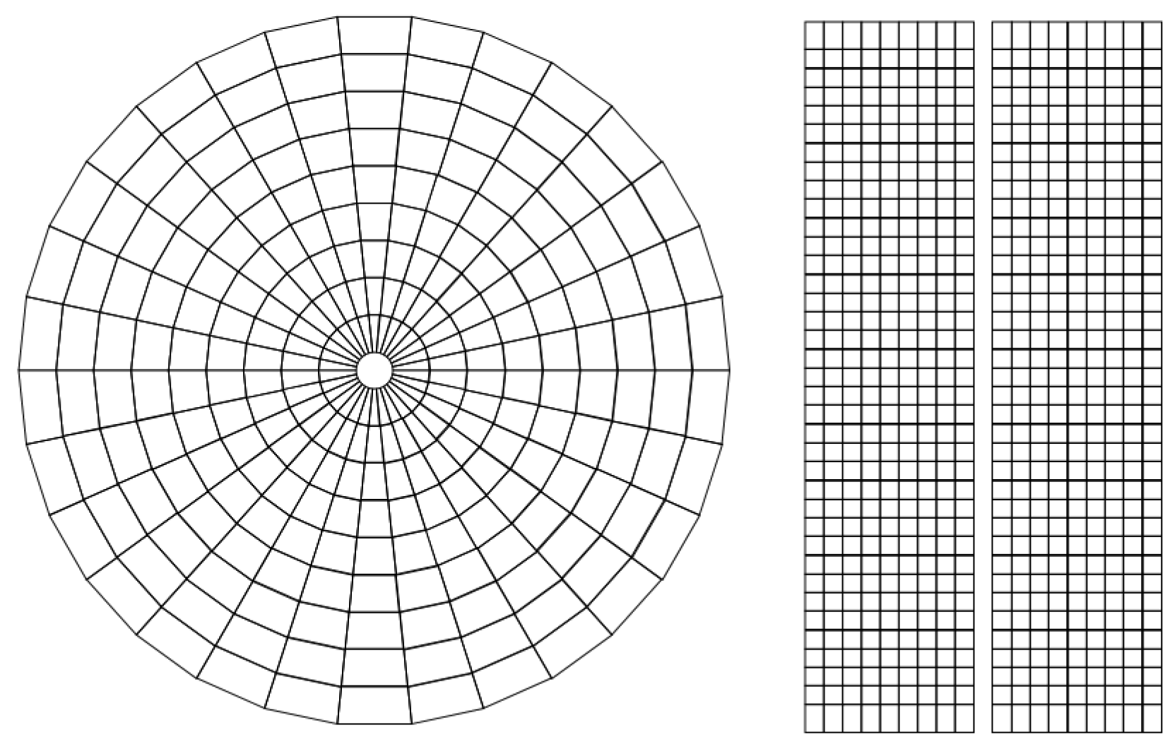
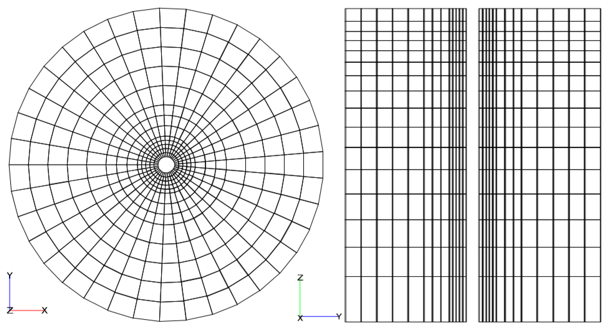
WFT is one of the most direct and effective methods used to confirm reservoir fluid properties and evaluate reservoirs in oil field exploration operations, playing an increasingly important role [11]. The enhanced formation dynamic tester (EFDT) is a modular, pump-extraction WFT instrument [12], designed for exploration and evaluation of wells to accomplish formation fluid sampling tasks. It provides various probe options for sampling operations, allowing for the construction of different probe combinations to establish a connection between the internal pipeline of the formation tester and the formation fluid. This facilitates pump-extraction sampling and pressure measurement; hydrocarbon purity calculation; and analysis of reservoir fluid properties, fluid interfaces, and reservoir properties [13]. Therefore, under the same instrument configuration conditions, the efficiency of pump-extracted sampling varies depending on the shape and distribution of the probes [14]. This study mainly focuses on probes such as the Small Type Inlet Probe, Middle Type Inlet Probe, Ellipse Type Inlet Probe, and Large Type Inlet Probe of the EFDT. Relevant parameters are shown in

Table 1. Parameters of Fluid Sampling Probes.

Type	Name	Inlet Area (in2)	Standard Ratio
S	Small Type Inlet Probe	0.21	0.27
M	Middle Type Inlet Probe	0.79	1
E	Ellipse Type Inlet Probe	2.32	2.94
L	Large Type Inlet Probe	6.23	7.89
3D-E	3D-Ellipse Type Inlet Probe	2.32 × 3	2.94 × 3

.

The standard ratio refers to the ratio of the suction area of other probes to that of the middle-type inlet probe. In addition, the 3D probe is achieved by combining a fluid sampling pump with greater efficiency. Based on the Small Type Inlet Probe, Middle Type Inlet Probe, Ellipse Type Inlet Probe, and Large Type Inlet Probe, three probes of the same type are selected to achieve the application of a 3D probe with a uniformly distributed radial orientation of 120 degrees and a combination of radial push-and-connect.

2.2. Meshing Model

Grid model generation technology serves as a link between physical and computational models for numerical simulation. Depending on whether the generated grid units have regularity, it can be divided into structured grids and unstructured grids [15]. The quality of grid generation has a significant impact on factors such as accuracy and efficiency in subsequent numerical simulation calculations, playing a crucial role in the numerical simulation process [16]. This paper primarily focuses on parameters such as the length and width of the probe suction mouth used in fluid pump-extraction sampling operations during WFT. Centered around the target operation well, a method for constructing a radial grid model with variable grid step length is developed. This method provides the spatial coordinates of each grid node and the connectivity of each grid node, supporting the implementation of the numerical simulation calculation model and providing a more detailed description of the operational process.

Therefore, in the process of dividing the three-dimensional spatial grid model, to simplify the calculation formula, it is assumed that the X and Y coordinates at the position of the wellbore center are both zero. The calculation formulas for the X and Y coordinates of the vertices of the grid model along the perimeter of the wellbore are shown in Equations (1) and (2).

$$x\left(i,j,k\right)=x^{\prime }cos(j\alpha -0.5\alpha )$$

(1)

$$y\left(i,j,k\right)=x^{\prime }sin(j\alpha -0.5\alpha )$$

(2)

where

$$x^{\prime }=\left(re+\sum \left(n\left(ii\right)-1\right)r_s\left(ii\right)\right)cos\left(0.5\alpha \right)$$

(3)

$$\alpha =360/nr$$

(4)

$$R=\left(re+\sum n\left(ii\right)r_s\left(ii\right)\right)$$

(5)

In the above formulas, $i$ denotes the azimuthal node number, $i=1,2\dots ,nc$, with $nc-1$ being the number of azimuthal grids; $j$ denotes the radial node number, with $nr-1$ being the number of radial grids; $k$ denotes the longitudinal node number, $k=\mathrm{1,2},\dots ,nk,\dots ,2nk+2$, with $2nk+1$ being the number of longitudinal grids; $\alpha$ represents the azimuthal partition baseline angle; $re$ denotes the wellbore radius; $ii$ represents the sequential number of the planar grid partition region; $n$ denotes the number of partitions corresponding to each region on the plane; $r_s$ represents the radial step length for each region; $R$ represents the modeling control radius, with the wellbore as the center on the plane. $x$ and $y$ represent the circumferential and radial vertex coordinates of the grid model plane, respectively. $x^{\prime }$ is the initial spatial coordinate of the vertex in different circumferential directions corresponding to the radial direction.

Furthermore, based on the depth $D$ where the probe is located, assuming the baseline node number of the longitudinal direction where the probe is located is used as the reference node, $k=nk$. The formula for calculating the longitudinal Z coordinate of the grid vertex with variable longitudinal step length is as follows:

$$z\left(i,j,k\right)=D-\left(2\left(nk-k+1\right)-1\right)h-∆D(nk-k+1)$$

(6)

where $k=1,\dots ,nk+1$.

$$D_T=z\left(i,j,1\right)$$

(7)

To construct grid nodes downward and achieve the calculation of the longitudinal Z coordinate of grid vertices with variable longitudinal step length, the formula is as follows:

$$z\left(i,j,k\right)=D-\left(2\left(nk-k+1\right)-1\right)h-∆D(nk-k+1)$$

(8)

where $k=nk+2,\dots ,2nk+2$.

$$D_B=z\left(i,j,2nk+2\right)$$

(9)

In the above formulas, $D$ represents the depth of the probe operation, $h$ denotes the reference grid thickness centered around the depth of the probe operation, $D_T$ represents the depth of the top of the target reservoir, and $D_B$ represents the depth of the bottom of the target reservoir. Based on the grid partitioning methods described above, both fixed-step and variable-step grid models are constructed, and the computed results are as follows:

In Figure 1, $R=3$, $re=0.15$, $nc=31$, $nr=10$, $h=0.05$, $∆D=0$, $nk=18$. In Figure 2, $R=3$, $re=0.15$, $nc=31$, $nr=10$, $h=0.05$, $∆D=0.02$, $nk=7$. The results show that the method described in this paper can produce a longitudinal fixed-step grid model when $∆D=0$, and a longitudinal variable-step grid model when $∆D\ne 0$.

Through the analysis of the two cases above, it is evident that the total number of grids generated by the grid model shown in Figure 1 is 9 × 30 × 37, while the total number of grids generated by the grid model shown in Figure 2 is 9 × 30 × 15. Compared to the fixed-step grid partitioning method, by controlling the relevant parameters of the variable step, not only can the control of local grid volume be achieved, but also the total number of grid model nodes can be reduced more effectively for subsequent numerical simulation calculations, thereby improving computational efficiency. Through controlling the step length of the planar partition area, overlaying longitudinal step parameters, and controlling the width of the probe suction mouth, it is more convenient to establish a three-dimensional wellbore reservoir grid model considering information such as the probe suction area, wellbore radius, and mud invasion range.

2.3. Numerical Simulation Model

In the field of fluid mechanics, finite difference, finite element, and finite volume methods are commonly used numerical techniques for solving partial differential equations [17]. The basic principle of the finite volume method (FVM) is to discretize the computational domain of the physical phenomenon described by the differential equations into discrete finite volume elements. Then, the integral of properties such as energy and mass is performed over each volume element to construct a discrete system of algebraic equations. The numerical solution is obtained by solving this system of equations [18]. FVM directly discretizes integral forms of conservation equations in physical space, making it suitable for arbitrary grid forms. One significant advantage is that it ensures fluid flow conservation within local grids while also handling complex boundary problems. Therefore, in the context of numerical simulation of fluid sampling in wireline formation testing, considering the heterogeneity of reservoirs around the well, centimeter-scale grid resolution, and irregular grid models, the integral equation for mass conservation is formulated as follows:

$${∯}_{s_e+s_i}\left(\sum V\right)ds+\sum Q={\iiint }_v∆(\varnothing \sum (S·\rho ))dv$$

(10)

In this equation, ${∯}_{s_e+s_i}\left(\sum V\right)ds$ represents the surface flux integral over the control volume, $\sum Q$ represents the volume integral of the source/sink terms, and ${\iiint }_v∆(\varnothing \sum (S·\rho ))dv$ represents the volume integral of the mass increment within the control volume.

To better understand the seepage during the pump extraction process, this study makes the following assumptions regarding the seepage of fluid into the probe during the wireline formation testing fluid sampling process, focusing on three main stages: pure water phase, oil–water mixed phase, and near-pure oil phase:

(a)

Three-Dimensional Two-Phase Black Oil Model: In this model, the invading formation mud and formation water are collectively referred to as the water phase, while the formation oil is the hydrocarbon phase. The two phases are immiscible and do not undergo chemical reactions.

(b)

Consideration of Various Factors: This includes the heterogeneity of the reservoir in both the horizontal and vertical planes, capillary pressure, gravity effects, rock compressibility, and fluid compressibility.

(c)

Boundary Conditions: The invading mud around the wellbore is water-based, and the initial invasion is an editable known condition. The outer boundary condition of the reservoir is a constant pressure boundary, while the inner boundary condition of the probe fluid sampling model is a constant liquid operation.

Using the finite volume method for spatial discretization and the backward Euler method for temporal discretization [19], the mass conservation discretized control equation with pressure as the solving parameter is formulated as follows:

$$\begin{array}{c}{\displaystyle \sum _{j=1}^{z\left(i\right)}}{T}_{ij}\left({\rho }_{wij}{\lambda }_{oj}^n+{\rho }_{oij}{\lambda }_{wj}^n\right)P_{h\left(i,j\right)}^{n+1}\hfill \\ \hspace{1em}\hspace{1em}\hspace{1em}\hspace{1em}\hspace{1em}\hspace{1em}-\left({\displaystyle \sum _{j=1}^{z\left(i\right)}}{T}_{ij}\left({\rho }_{wij}{\lambda }_{oj}^n+{\rho }_{oij}{\lambda }_{wj}^n\right)+{\displaystyle \frac{V{\varphi }_i{\rho }_{oi}{\rho }_{wi}\left(c_o{S}_o^n+c_w{S}_w^n+c_f\right)}{\Delta t}}\right)P_i^{n+1}\hfill \\ \hspace{1em}\hspace{1em}\hspace{1em}\hspace{1em}\hspace{1em}\hspace{1em}=-g\left({\displaystyle \sum _{j=1}^{z\left(i\right)}}{T}_{ij}\Delta D_{ij}{\rho }_{wij}{\rho }_{oij}\left({\lambda }_{oj}+{\lambda }_{wj}\right)\right)\hfill \\ \hspace{1em}\hspace{1em}\hspace{1em}\hspace{1em}\hspace{1em}\hspace{1em}+{\displaystyle \sum _{j=1}^{z\left(i\right)}}{T}_{ij}{\rho }_{oij}{\lambda }_{wj}^n\left(P_{cowj}^n-P_{cowi}^n\right)-\left({\displaystyle \frac{V{\varphi }_i{\rho }_{oi}{\rho }_{wi}\left(c_o{S}_o^n+c_w{S}_w^n+c_f\right)P_i^n}{\Delta t}}\right)\hfill \\ \hspace{1em}\hspace{1em}\hspace{1em}\hspace{1em}\hspace{1em}\hspace{1em}-Q\hfill \end{array}$$

(11)

In the above equation: $T$ is the transmissibility between the connected grid blocks, $T={\displaystyle \frac{1}{T_i+T_j}}$, $T_i={\displaystyle \frac{L}{A·NTG·K·d}}$; $A$ is the contact area of the current grid block in different connected directions; $L$ is the distance from the center of the current grid block to different contact surfaces; $NTG$ is the effective thickness ratio; $K$ is the permeability; $d$ is the probe area ratio coefficient, where $d=1$ for grid blocks not in contact with the probe inlet, and $d={\displaystyle \frac{A_p}{A_c}}$ for grid blocks in contact. $A_p$ is the probe inlet area, $A_c$ is the contact area of the grid block in operation; $n$ is the time-step coefficient; $i,j$ are the indices of grid blocks with a connection relationship; $z\left(i\right)$ is the total number of grid connections for the current grid block $i$; ${\lambda }_o={\displaystyle \frac{k_{ro}}{{\mu }_o}}{\rho }_o$, ${\lambda }_w={\displaystyle \frac{k_{rw}}{{\mu }_w}}{\rho }_w$, $k_{ro}$ is the relative permeability of the hydrocarbon phase; $k_{rw}$ is the relative permeability of the water phase; ${\rho }_o$ is the density of the hydrocarbon phase fluid; ${\rho }_w$ is the density of the water phase fluid; ${\mu }_o$ is the viscosity of the hydrocarbon phase fluid; ${\mu }_w$ is the viscosity of the water phase fluid; $\varphi$ is the porosity; $P$ is the pressure; $V$ is the grid block volume; $c_o$ is the compressibility of the hydrocarbon phase fluid; $c_w$ is the compressibility of the water phase fluid; $c_f$ is the comprehensive compressibility; $\Delta D$ is the depth difference between grid blocks; $\Delta t$ is the iterative time step size, when dealing with situations where the grid cell volume is too small or the model is quite complex, resulting in non-convergence during the solving process; convergence optimization can be achieved by reducing this value. $g$ is the gravitational acceleration; $Q$ is the total sampling fluid rate at the probe, with $Q=0$ in the pressure equation for grid blocks not in contact with the probe.

The water phase saturation model for solving the above equation is given by

$$S_{wi}^{n+1}=S_{wi}^n+{\displaystyle \frac{\Delta t\left({\sum }_{j=1}^{z\left(i\right)}{T}_{ij}{\lambda }_{wij}\left(P_{wj}^{n+1}-P_{wi}^{n+1}+{\rho }_{wij}g\Delta D_{ij}\right)+q_w\right)-V{\phi }_i{S}_{wi}^n\Delta P_{wi}^{n+1}{\rho }_{wi}\left(c_w+c_f\right)}{V{\phi }_i{\rho }_{wi}}}$$

(12)

$$S_{oi}^{n+1}=1-S_{wi}^{n+1}$$

(13)

where $S_w$ is the water phase saturation and $S_o$ is the hydrocarbon phase saturation.

Other major auxiliary equations include the following:

Relative permeability model:

$$K_{rw}=K_{rw}\left(S_w\right)$$

(14)

$$K_{ro}=K_{ro}\left(S_w\right)$$

(15)

Capillary pressure model:

$$P_{cow}=P_o\left(S_w\right)-P_w\left(S_w\right)$$

(16)

Mud invasion into the formation:

$$S_w={S(x,y,z)}_{t=0}$$

(17)

The effective thickness ratio of the formation:

$$NTG={NTG(x,y,z)}_{t=0}$$

(18)

The porosity of the formation:

$$\varphi ={\varphi (x,y,z)}_{t=0}$$

(19)

The permeability of the formation:

$$K={K(x,y,z)}_{t=0}$$

(20)

where $K_{ro}$ is the relative permeability of the hydrocarbon phase, $K_{rw}$ is the relative permeability of the water phase, $t=0$ represents the initial time state, $P_{cow}$ is the capillary pressure, $P_o$ is the hydrocarbon phase pressure, $P_w$ is the water phase pressure, $NTG$ is the effective thickness ratio, $\varphi$ is the porosity, and $K$ is the permeability.

The main advantage of the finite volume method is its good adaptability to irregular and complex seepage simulation calculations, as well as its ability to handle complex physical phenomena such as phase change and multiphase flow occurring within the computational domain. Firstly, the computational domain can be divided into several non-overlapping control volumes or flow cells. Secondly, the mass conservation equations for each control volume or flow cell are discretized. Finally, using the discretized forms of the equations obtained, in conjunction with matrix solution methods, the numerical solution for reservoir water saturation and formation pressure distribution during the fluid sampling operation process is computed.

2.4. Target Parameter Calculation Model

The calculation of hydrocarbon content during the wireline formation testing process while drilling plays a crucial role in reservoir analysis, productivity assessment, and implementation of operational measures. Therefore, to obtain the hydrocarbon content and flow pressure during the wireline formation testing process while drilling, considering factors such as skin factor and probe-to-grid contact area ratio coefficient, this paper integrates the pump rate. Based on spherical flow, the model for calculating flow pressure and hydrocarbon content at the probe inlet is constructed as follows:

The calculation model for hydrocarbon content in the fluid at the probe inlet:

$$f_w={\displaystyle \frac{1}{1+\frac{u_w}{u_o}\cdot \frac{k_{ro}}{k_{rw}}}}$$

(21)

$$q_w=Q\times f_w$$

(22)

$$q_o=Q-q_w$$

(23)

$$f_o={\displaystyle \frac{q_o}{Q}}$$

(24)

The calculation model for the flow pressure at the probe inlet:

$$P_{wf}={\displaystyle \frac{q_o}{G_o}}+P_o$$

(25)

The $G_o$ solution model is as follows:

$$G_o={\displaystyle \frac{2\pi {Kk}_{ro}hd}{{\mu }_o\left(ln\left(\frac{r_e}{r_w}\right)+s\right)}}$$

(26)

where $f_w$ represents the water phase fluid content ratio; $f_o$ represents the hydrocarbon phase fluid content ratio; $q_w$ is the flow rate of the water phase fluid; $q_o$ is the flow rate of the hydrocarbon phase fluid; $P_{wf}$ is the flowing pressure at the probe inlet; $G_o$ is the comprehensive characterization coefficient; $r_e$ is the wellbore radius; $r_w$ is the effective fluid supply radius of the wellbore; and $s$ is the probe skin factor, which is dimensionless.

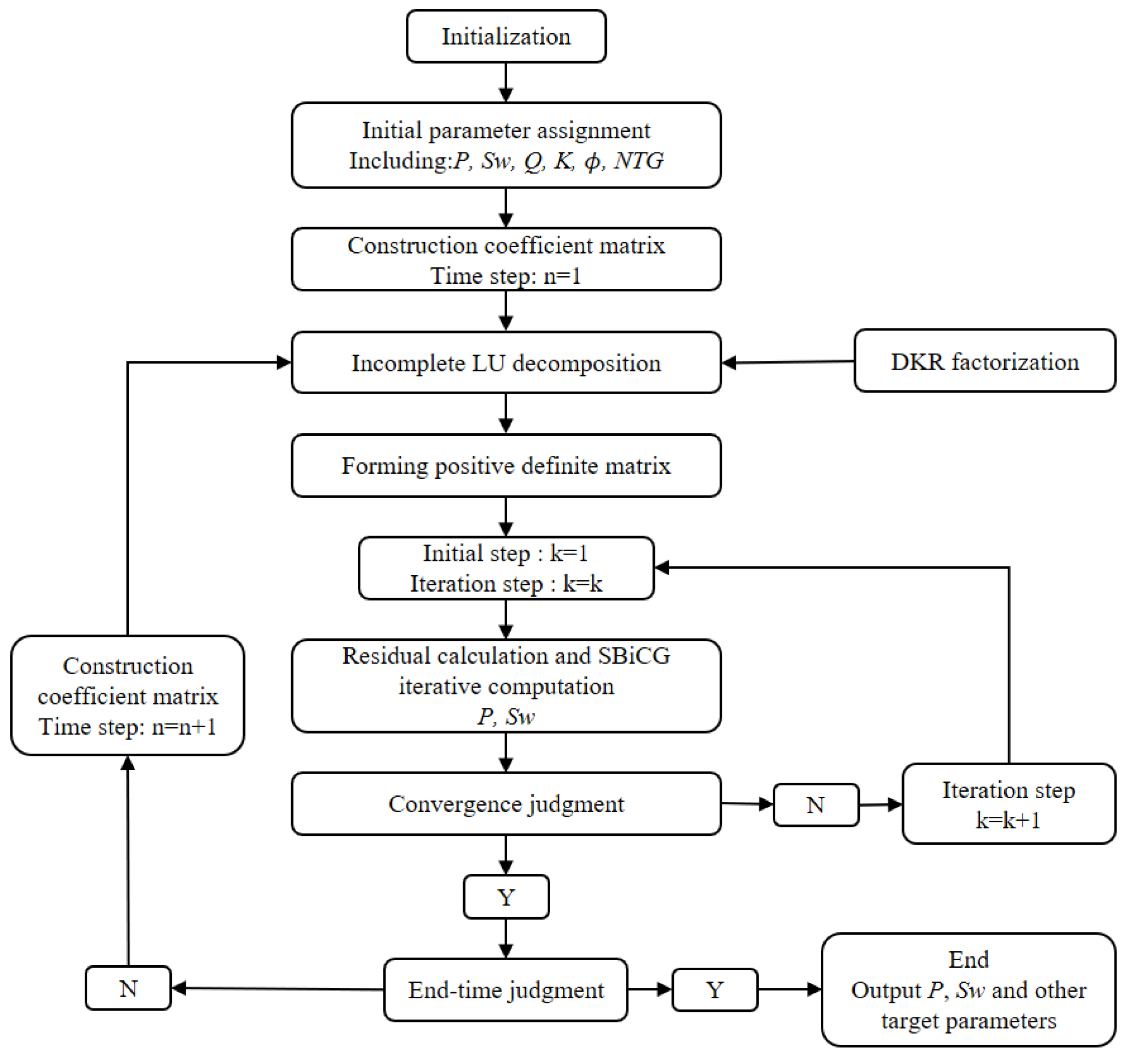
2.5. Solving Matrix Equation

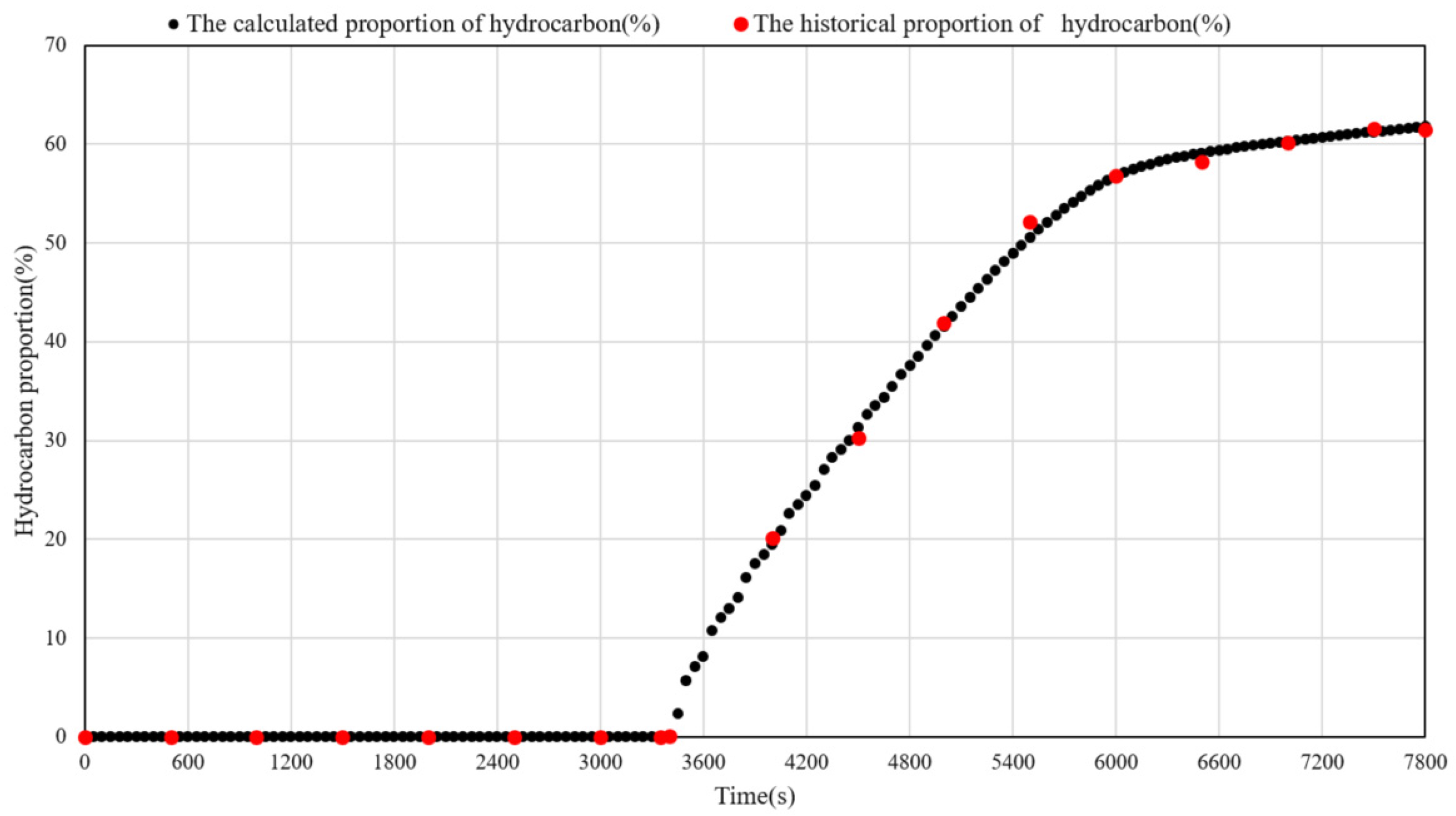
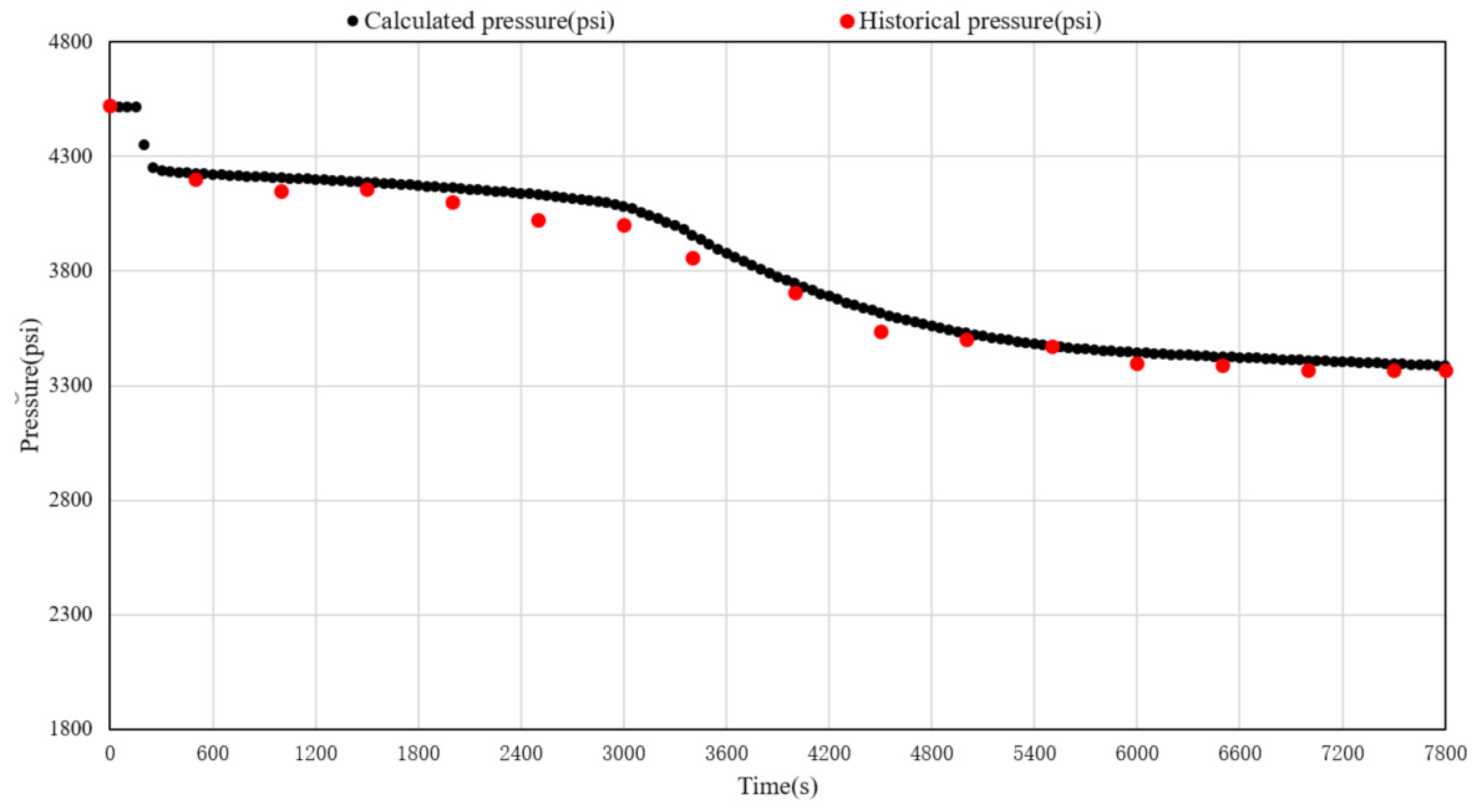
The calculation of hydrocarbon content during the wireline formation testing process while drilling plays a crucial role in reservoir analysis, productivity assessment, and implementation of operational measures. Therefore, to obtain the hydrocarbon content and flow pressure during the wireline formation test, the following method is used.

The Stabilized BiConjugate Gradient (SBiCG) method is an iterative technique used to solve linear systems of equations with asymmetric matrices (Ax = b). In comparison to the conventional BiConjugate Gradient (BiCG) method, SBiCG introduces additional step parameters and a modified inverse preconditioner, leading to faster convergence rates and improved numerical stability [20]. Therefore, this paper primarily adopts the matrix pre-processing SBiCG solution method based on incomplete LU decomposition for solving pressure equations and saturation. The main steps of the solution process are outlined as shown in Figure 3.

The basic idea of the SBiCG iterative method is to maintain the orthogonality of vectors during the iteration process while using appropriate step parameters to enhance the convergence speed. This method first computes two conjugate directions and then uses them to generate two new search directions. These directions remain orthogonal to previous search directions, and new iterative solutions are generated using step parameters.

It also employs a modified inverse preconditioner. The modified inverse preconditioner utilizes an additional step parameter to balance the effects of preconditioning and incomplete LU decomposition. This helps prevent the accumulation of rounding errors in the preconditioner during the iteration process and aids in maintaining the orthogonality of search directions.

In the numerical simulation model solving process, SBiCG is an efficient method for solving asymmetric matrix linear systems of equations. It can maintain the orthogonality of search directions while achieving good numerical stability and rapid convergence speed. By characterizing the fluid seepage characteristics of the grid model and utilizing the computed pressure field values at each time step, combined with Equations (12) and (13) mentioned above, the calculation of reservoir water and hydrocarbon saturation distributions can be further completed. Through calculation models such as those for phase permeability, hydrocarbon content, and flow pressure, the calculation of hydrocarbon phase fluid proportion and pressure is accomplished, providing important technical support for the design of WFT fluid sampling operations, process optimization analysis, and indicator prediction during drilling operations.

2.6. Model Analysis

To analyze the computational effectiveness of the WFT fluid sampling process numerical simulation model, numerical simulations were performed considering the pump-extraction sampling process of an elliptical probe with water-based drilling fluid invading the reservoir. A comprehensive analysis of the method’s applicability was conducted by fitting and comparing the simulation results with measured data. The relevant basic parameters are shown in

Table 2. Basic parameters of model.

Porosity (%)	Permeability (MD)	Hole Diameter (m)	Initial Pressure (psi)	Invasion Depth (m)	Ratio of Effective Thickness (m/m)
15.7	25	0.1556	4520.95	0.85	0.912

and

Table 3. Liquid parameters of model.

Drilling Fluid Viscosity (mPa·s)	Formation Fluid Viscosity (mPa·s)	Drilling Fluid Density (g/cm3)	Formation Fluid Density (g/cm3)
0.55	2.50	1.01	0.903

, and the experimental data for the relative permeability curves are presented in

Table 4. Fluid relative permeability experimental data.

Water Saturation (%)	Hydrocarbon Relative Permeability (-)	Water Relative Permeability (-)
0	1	0
32	0.88	0
35	0.82	0.01
45	0.50	0.12
52	0.30	0.25
60	0.10	0.48
65	0.02	0.61
70	0.01	0.71
80	0	0.88

.

By considering the starting depth of 3286.8 m and the ending depth of 3287.8 m, with the probe located at a depth of 3286.9 m, the grid longitudinal thickness is set to 0.026 m, and the longitudinal overlapping step is 0.005 m. The planar modeling radius is 3 m, with 37 radial grid divisions. The plane is divided into three regions with boundaries at 0.55 m, 1.15 m, and 3 m, with division counts of 5, 3, and 5, respectively. The grid model construction is shown in Figure 4.

Based on the known water-based mud invasion depth of 0.85 m, by fitting the actual measured hydrocarbon phase fluid proportion and pressure with the computed results, the initial distribution of water phase saturation within the invasion range is set as shown in Figure 5 below.

The numerical simulation results compared with historical measured results are shown in Figure 6 and Figure 7.

In this calculation process, the water phase compressibility is 0.000015 bar⁻¹, and the hydrocarbon phase compressibility is 0.000144 bar⁻¹. The probe operating depth is 3286.9 m, and the total operating duration is 7880 s. The actual fluid sampling speed for the first 200 s averages 0.1 cc/s, and from 200 s onward, it is 4.38 cc/s. The monitored pressure difference at the end of the actual operation is 1154.82 psi, with the hydrocarbon breakthrough time observed at 3400 s. Compared with the calculation results, the average fitting rate for the hydrocarbon fluid proportion is 98.5%, the average fitting rate for the pressure curve is 98.67%, and the final simulated operation production pressure difference is 1133.05 psi, with a fitting rate of 98.11%.

Therefore, it is evident from the results that a satisfactory computational performance has been achieved. This analysis holds significant guidance for activities such as analyzing the factors affecting WFT pump extraction, predicting hydrocarbon content, selecting probes, and optimizing pump extraction operations in drilling processes.

3. Results and Discussion

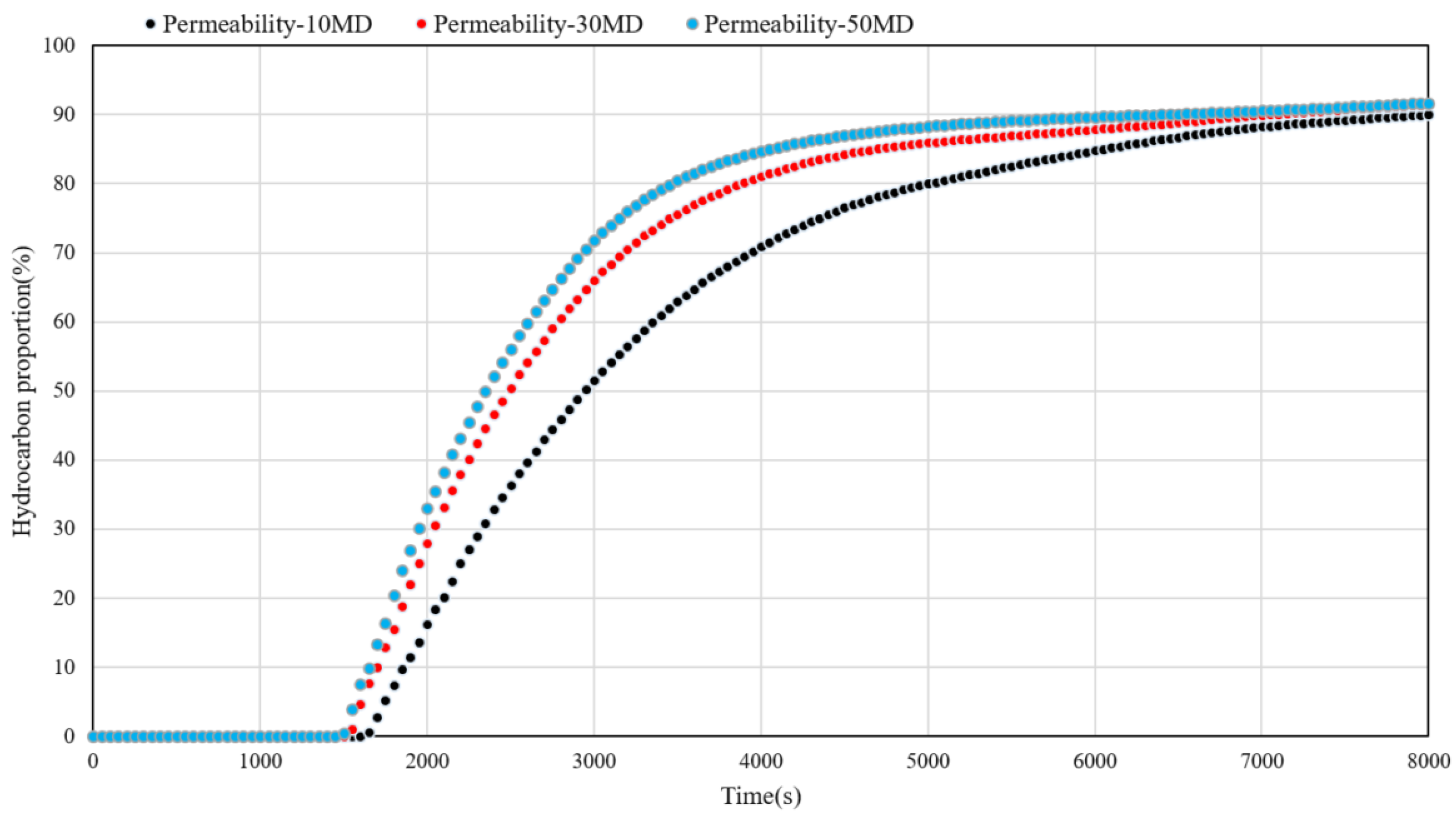
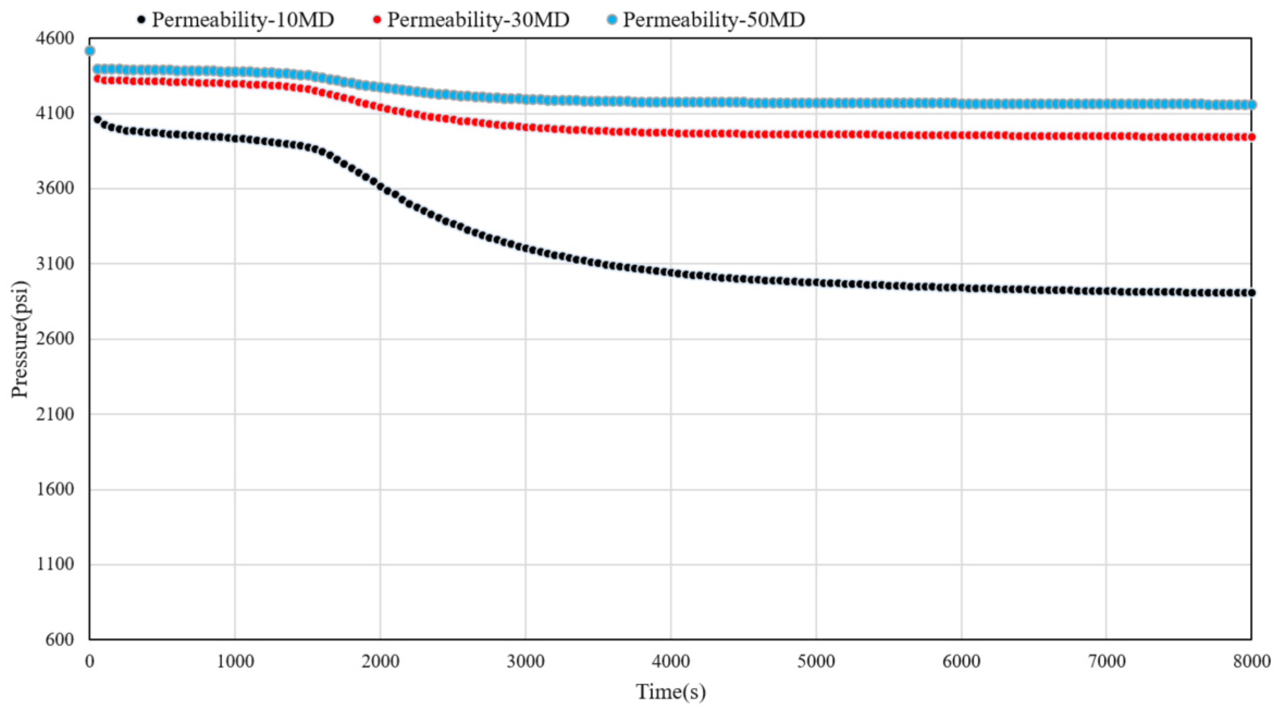
3.1. Parameter Sensitivity Analysis

First, based on the reservoir and fluid property parameters of the aforementioned numerical simulation model, a sensitivity study was conducted on factors such as reservoir permeability and fluid sampling operation speed. With a water-based mud invasion depth of 0.4 m, a water phase saturation of 100% within the invasion range, and a longitudinal grid step length of 0.02 m, two types of simulation scenarios were set up:

(a)

For elliptical probe operation at a sampling speed of 4 cc/s with permeability of 10 MD, 30 MD, and 50 MD.

(b)

For the same permeability of 30 MD with sampling speeds of 3 cc/s, 4 cc/s, and 5 cc/s.

Key indicators such as hydrocarbon proportion and pressure curves were calculated and analyzed. The aim was to explore the response characteristics of key parameters like hydrocarbon content and pressure during the fluid sampling process under different reservoir permeability and sampling speed conditions. The calculation results are shown in Figure 8, Figure 9, Figure 10 and Figure 11 below.

In summary, it can be seen that reservoir permeability significantly affects bottom hole pressure during the sampling operation. As shown in Figure 8 and Figure 10, higher reservoir permeability increases the Poisson ratio of hydrocarbon flow, resulting in a higher hydrocarbon sampling rate per unit time and better fluid permeability. Reasonably increasing the sampling speed can help accelerate the flow of hydrocarbon fluid from the reservoir to the sampling probe.

Furthermore, as shown in Figure 9 and Figure 11, higher reservoir permeability requires a smaller production pressure differential during the sampling process. This indicates that less energy is needed to create effective bottom-hole pressure, thereby reducing the difficulty of fluid sampling and improving the breakthrough time and operational efficiency of wireline fluid sampling for hydrocarbon fluids. Conversely, if the reservoir permeability is relatively low, the hydrocarbon fluid permeability is poor. In this case, the WFT operation pump requires higher power to provide a greater production pressure differential, forming higher pressure energy at the bottom-hole sampling point, thus facilitating the outflow of hydrocarbon fluid.

Therefore, for WFT fluid sampling operations in high-permeability reservoirs, increasing the pump speed under reasonable operational pressure differentials and maximum pump efficiency can help quickly extract hydrocarbon fluids from the reservoir. In low-permeability reservoirs, reducing the pump speed within a reasonable pump efficiency range can help maintain a stable operational pressure differential.

Evaluating the fluid sampling process for different permeability reservoirs provides direct and quantifiable guidance for assessing the effectiveness of operational measures during WFT fluid sampling. This approach offers practical insights for optimizing sampling operations in varying reservoir conditions.

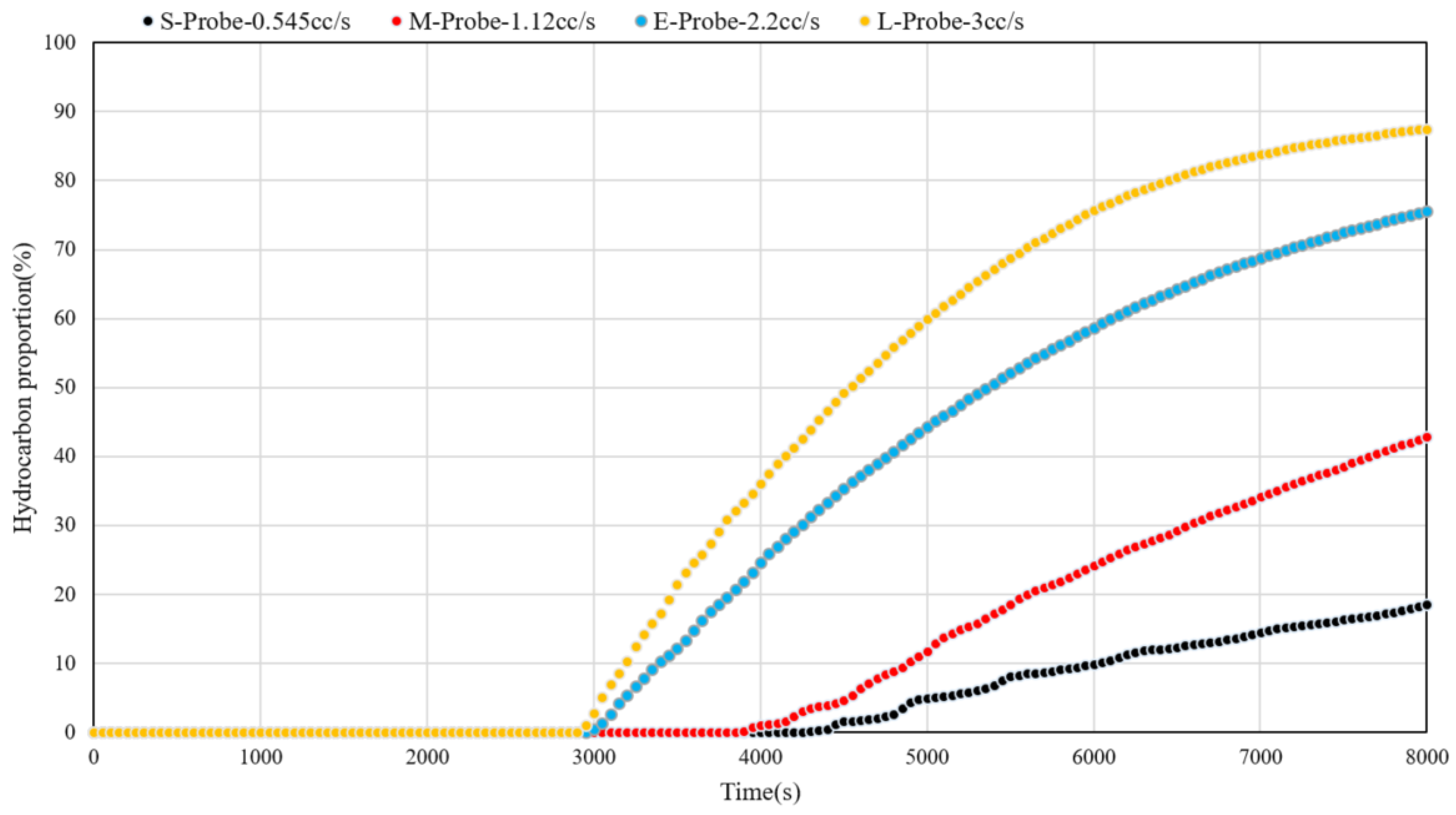
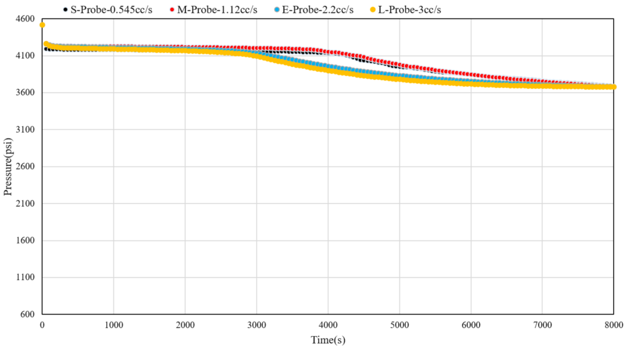
3.2. Probe Operation Analysis

Secondly, this study examines the operational effectiveness of probes with different inlet sizes during fluid sampling processes to provide technical support for probe selection. Specifically, under a reservoir permeability of 10 MD, with a fluid sampling operation time of 8000 s and a final pressure differential of 841.15 psi, we analyzed the fluid sampling performance of four different inlet-sized probes.

Under the same operational pressure differential, the pump operation speeds were as follows: Small Type Inlet Probe at 0.545 cc/s, Middle Type Inlet Probe at 1.12 cc/s, Ellipse Type Inlet Probe at 2.2 cc/s, and Large Type Inlet Probe at 3 cc/s. The effectiveness of different pump operation measures is illustrated in the following Figure 12 and Figure 13.

This indicates that in low-permeability reservoirs, different types of probes, due to variations in the size of their inlet areas and the influence of pump extraction speed, exhibit differences in the time it takes to first encounter hydrocarbons. Under the known minimum control requirements for production pressure drop based on pump efficiency, probes with larger inlet areas tend to encounter hydrocarbons earlier during fluid sampling. Additionally, they extract a greater volume of hydrocarbon phase fluid within the same duration, indicating higher operational efficiency. Particularly in environments with lower permeability reservoirs, probes with larger inlet areas demonstrate a more pronounced advantage in operational efficiency under feasible pressure drop conditions. This aligns with the requirements of field production operations.

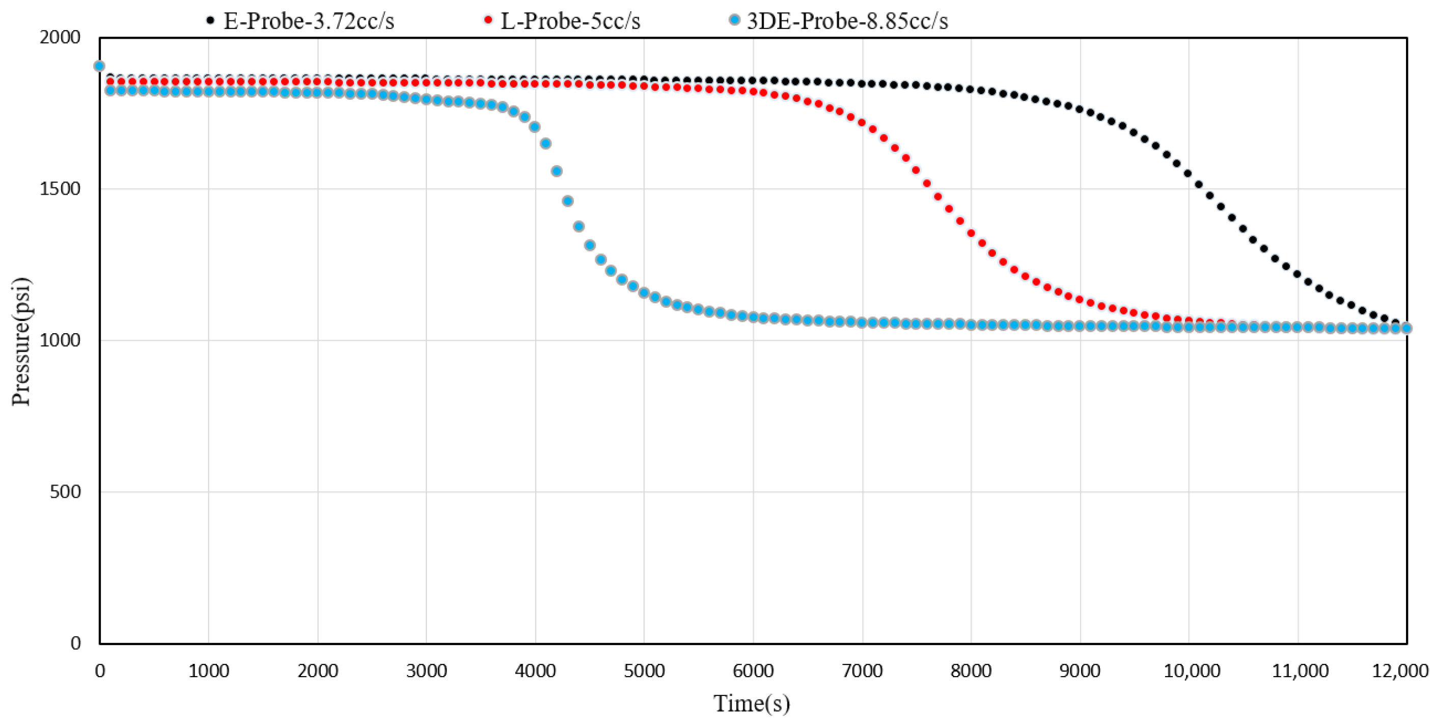
3.3. Sampling Operations in Shallow Heavy Oil Formations

For a certain offshore heavy oil block characterized by high viscosity, high density, and high colloidal content, field experiments have shown that a lack of reasonable external force during fluid sampling can lead to difficulties such as the inability of oil samples to flow out of the sampling bucket and excessive pressure drop. Additionally, the reservoir in this area is loosely cemented, with weak bonding between sand grains, making sand detachment-prone under large pressure gradients. Therefore, in an effective fluid sampling process, it is necessary not only to ensure efficient fluid sampling but also to avoid instrument blockage due to sanding.

Taking Well A in this block as an example, the fluid viscosity of the sampled crude oil in the formation is 43 mPa·s, density 9.15 g/cm³, permeability 500 MD, porosity 22%, NTG 64%, probe sampling depth 1362.2 m, reference pressure 1904.34 psi, maximum controlled pressure differential for effective operation is 900 psi, maximum pump efficiency extraction rate is 9 cc/s, and sampling duration is 12,000 s. For three operation schemes involving elliptical probe operation (sampling speed 3.72 cc/s), large-suction probe operation (sampling speed 5 cc/s), and 3D elliptical probe operation (sampling speed 8.85 cc/s), optimization analysis and evaluation of probe selection and sampling efficiency in the WFT process of shallow heavy oil reservoirs were conducted. After numerical simulation calculations for different schemes, the hydrocarbon phase proportion and pressure curve calculation results for each operation scheme were as follows (Figure 14 and Figure 15):

In this analysis, based on the sampling operation target depth of the water-based mud invasion depth of 0.3 m into the reservoir, with a saturation of 100% within the invasion range, longitudinal grid division with an equal step length of 0.03 m was conducted. The depth range of the formation was from 1361.8 m to 1362.6 m, with a wellbore radius of 0.15 m, and a radial grid division of 31. The modeling radius in the plane was 3 m. Three regions were defined in the plane circumferentially, with boundary distances of 0.45 m, 1.45 m, and 3 m, and respective divisions of 2, 4, and 4. While ensuring effective control of the maximum operating pressure differential, pump efficiency, and sampling speed, simulated analyses of operational measures were conducted. Within the same implementation period of 12,000 s for the operation, the simulated final pressure differential for the three schemes shown in Figure 15 was 870 psi, meeting the condition of a maximum operating pressure differential of 900 psi.

Furthermore, by setting the hydrocarbon phase fluid proportion greater than 0.4% as the breakthrough threshold and 80% as the compliance analysis threshold, a timeliness analysis was conducted for elliptical probe operation, large-suction probe operation, and 3D elliptical probe operation. The statistical results are presented in

Table 5. Statistical results for the aging time.

	Sampling Speed (cc/s)	Operating Time Hydrocarbon > 0.4% (s)	Operating Time Hydrocarbon > 80% (s)
E-Probe	3.72	7800	11,900
L-Probe	5.00	6000	8800
3D-E-Probe	8.85	3700	4900

below.

According to the statistical results in Table 5, under the same operating pressure difference conditions, the 3D elliptical probe fluid sampling process can achieve higher-speed fluid sampling operations. Compared to the other two types of probes, it can achieve hydrocarbon fluid breakthrough more quickly (hydrocarbon >0.4%), taking only 4900 s to achieve a hydrocarbon fluid purity of over 80%. Furthermore, under the operating pressure difference range of maximum pump efficiency, the 3D elliptical probe operation has improved breakthrough time by 2300 s and 3100 s compared to elliptical probe operation and large suction nozzle probe operation, and the compliance time has been improved by 3900 s and 7000 s. The efficiency of fluid sampling with the 3D probe is significantly better than with the other two single-suction nozzle probe operation modes. Additionally, combined with Figure 14, it can be observed that after reaching the breakthrough time, the amount of hydrocarbon-phase fluid sampled per unit time with the 3D probe operation is far superior to that of the other two probes, and it is more conducive to extracting more hydrocarbon-phase fluid under stable pressure difference conditions.

Furthermore, for the two single-suction nozzle probe operations, if the sampling speed is increased, it will face the risk of insufficient pump efficiency, significant pressure drop, large operating pressure differences, and instrument blockage due to sand production from the reservoir. Therefore, operating the 3D probe during the sampling of shallow heavy oil reservoirs can reduce pressure differences, increase flow area, ensure more crude oil flows out of the formation, improve fluid sampling efficiency, reduce the risk of instrument blockage due to sand production, and optimize pump-assisted fluid sampling efficiency, thereby enhancing timeliness with satisfactory results.

4. Conclusions

The present study unveils an advanced numerical simulation technology grounded in the finite volume method, designed to optimize fluid sampling operations within WFT during drilling endeavors. It elucidates various key techniques, spanning from meshing methodologies to numerical simulation modeling, matrix equation resolution, and the analysis of influential factors. By integrating these methodologies with empirical case data, a thorough analysis of operational efficacy is conducted. The primary conclusions drawn from this investigation are as follows:

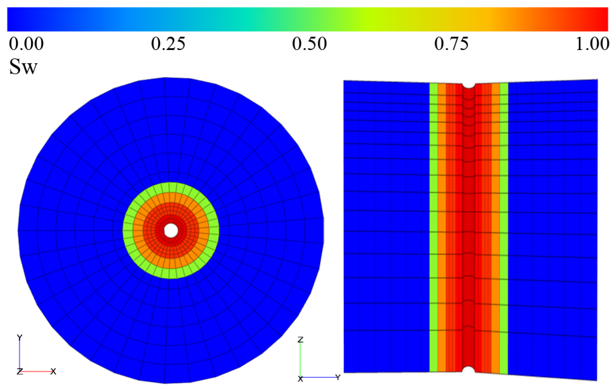
• Combining the variable step-size radial grid division technique considering the wellbore radius and the probe suction mouth size, a reasonable representation of the matching between the probe suction mouth and the grid model contact area can be achieved. By adopting a variable step-size grid model, it not only represents the permeation characteristics of the formation fluid into the sampling probe in a reasonable manner, but also reduces the overall number of grid models. This approach has a positive impact on the stability and timeliness of subsequent numerical simulation calculations.
• Based on the principles of the finite volume method and considering the influence of the ratio of the probe suction area to the contact area of the geological formation grid, a numerical simulation model for fluid sampling in WFT was constructed. This model can incorporate conditions such as probe type and mud invasion. Additionally, by using incomplete LU decomposition matrix preprocessing and SBiCG, the rapid solution of model target parameters was achieved. The validation and comparison of simulated calculation results with actual sampling data were completed, providing important support for the optimization design of WFT operations during drilling processes.
• Combining the numerical simulation model, sensitivity analysis of key information such as reservoir permeability, fluid sampling speed, and probe type was conducted. This further verified the response characteristics of calculation result curves such as the hydrocarbon phase ratio and pressure in different operational measures during fluid sampling processes under various permeability, fluid sampling speed, and probe type environments. Hence, reliable bases were provided for analyzing factors affecting the efficiency of WFT fluid sampling, in conjunction with reservoir properties and fluid characteristics.
• Addressing the optimization design requirements for fluid sampling operations in shallow heavy oil sand-bearing formations, the challenges faced in environments characterized by high viscosity, high density, and high colloidal content of heavy oil reservoirs were analyzed. These challenges include difficulties such as oil sample failure to flow out of the sampling bucket, excessive pressure drop during operations, and instrument clogging due to sand production. A comparative analysis was conducted between 3D probes and traditional single-suction probes, demonstrating advantages such as increased flow area and enhanced hydrocarbon phase fluid sampling under low-pressure differential operational requirements. This approach can effectively prevent instrument clogging caused by high-pressure gradients.

References

1. John, A.; Agarwal, A.; Gaur, M.; Kothari, V. Challenges and opportunities of wireline formation testing in tight reservoirs: A case study from Barmer Basin, India. J. Pet. Explor. Prod. Technol. 2017, 7, 33–42. [Google Scholar] [CrossRef]
2. Liu, H.; Wu, L.; Wang, M.; Zhang, H.; Qin, X. Calculation of depth of mud filtrate invasion based on formation sampling. J. Southwest Pet. Univ. (Sci. Technol. Ed.) 2023, 45, 97–106. [Google Scholar]
3. Liu, M.; Song, Y.; Jiang, Y.; Jiao, L. Application of wireline formation tester in moderate and low permeability depleted zones. Well Logging Technol. 2023, 47, 764–771. [Google Scholar]
4. Wang, X.; Zhou, C.; Wang, C.; Cao, W. Review on application of the wireline formation tester. Prog. Geophys. 2008, 23, 1579–1585. [Google Scholar]
5. Zhou, B.; Mo, X.; Tao, G. the numerical simulation of wireline formation tester with finite element method. J. Jilin Univ. Earth Sci. Ed. 2007, 37, 629–632. [Google Scholar]
6. Wang, C.; Cao, W.; Wang, X. Pressure gradient computation and application of the wireline formation tester. Pet. Explor. Dev. 2008, 35, 476–481. [Google Scholar] [CrossRef]
7. Alpak, F.O.; Torres-Verdín, C.; Habashy, T.M. Estimation of in-situ petrophysical properties from wireline formation tester and induction logging measurements: A joint inversion approach. J. Pet. Sci. Eng. 2008, 63, 1–17. [Google Scholar] [CrossRef]
8. Noirot, M.; Massonnat, G.; Jourde, H. On the use of Wireline Formation Testing (WFT) data: 2. Consequences of permeability anisotropy and heterogeneity on the WFT responses inferred flow modeling. J. Pet. Sci. Eng. 2015, 133, 776–784. [Google Scholar] [CrossRef]
9. Zhao, Y.; Ge, S.; Han, C.; Bie, K.; Shuai, S. Oil-gas sampling purity prediction based on numerical simulation for modular dynamic formation tester. Well Logging Technol. 2020, 44, 534–538, 552. [Google Scholar]
10. Zhou, Q.; Wu, L.; Qin, X. Applicable conditions of wireline formation testing instrument. Pet. Geol. Eng. 2022, 36, 115–118. [Google Scholar]
11. Xu, J.; Lv, H.; Cui, Y. An application analysis of wireline formation test in Bohai region. China Offshore Oil Gas 2008, 20, 106–110. [Google Scholar]
12. Ma, J. Application of EFDT in sand producing formation sampling. China Pet. Chem. Stand. Qual. 2019, 39, 53–54. [Google Scholar]
13. Zhao, C. Sampling probe optimization technology of the double hanging instrument for Wireline Formation Testing. Offshore Oil 2022, 42, 59–64. [Google Scholar]
14. Wu, L.; Liu, H.; Wang, M. Research on EFDT working system optimization and applicability. Petrochem. Technol. 2019, 26, 342–343. [Google Scholar]
15. Anderson, J.T.; Williams, D.M.; Corrigan, A. Surface and hypersurface meshing techniques for space–time finite element method. Comput.-Aided Des. 2023, 163, 103574. [Google Scholar] [CrossRef]
16. Busto, S.; Dumbser, M.; Río-Martín, L. An Arbitrary-Lagrangian-Eulerian hybrid finite volume/finite element method on moving unstructured meshes for the Navier-Stokes equations. Appl. Math. Comput. 2023, 437, 127539. [Google Scholar] [CrossRef]
17. Van der Vegt, J.J.; Van der Ven, H. Space–time discontinuous Galerkin finite element method with dynamic grid motion for inviscid compressible flows. J. Comput. Phys. 2002, 182, 546–585. [Google Scholar] [CrossRef]
18. Riemslagh, K.; Vierendeels, J.; Dick, E. Arbitrary Lagrangian-Eulerian finite-volume method for the simulation of rotary displacement pump flow. Appl. Numer. Math. 2000, 32, 419–433. [Google Scholar] [CrossRef]
19. Lv, X.; Huang, C.; Zhao, J. Numerical simulation of water flooding development of heterogeneous carbonate reservoir. J. Xi’an Shiyou Univ. (Nat. Sci. Ed.) 2016, 31, 75–81. [Google Scholar]
20. Van der Vorst, H.A. Bi-CGSTAB: A fast and smoothly converging variant of Bi-CG for the solution of nonsymmetric linear systems. SIAM J. Sci. Stat. Comput. 1992, 13, 631–644. [Google Scholar] [CrossRef]
Figure 1. Fixed step length grid division in plane and longitudinal directions.
Processes 12 01515 g001
Figure 2. Variable step length grid division in plane and longitudinal directions.
Processes 12 01515 g002
Figure 3. Schematic diagram of the calculation process of the numerical simulation.
Processes 12 01515 g003
Figure 4. Numerical simulation grid model division.
Processes 12 01515 g004
Figure 5. Initial distribution of water phase saturation due to mud invasion.
Processes 12 01515 g005
Figure 6. Comparison of historical and calculated hydrocarbon proportion.
Processes 12 01515 g006
Figure 7. Comparison of historical and calculated pressures.
Processes 12 01515 g007
Figure 8. Results for hydrocarbon proportion at the same speed with different permeabilities.
Processes 12 01515 g008
Figure 9. Results for pressure at the same speed with different permeabilities.
Processes 12 01515 g009
Figure 10. Results for hydrocarbon proportion at different speeds with the same permeability.
Processes 12 01515 g010
Figure 11. Results for pressure at different speeds with the same permeability.
Processes 12 01515 g011
Figure 12. Results for hydrocarbon proportion during operations with different probes at the same differential pressure.
Processes 12 01515 g012
Figure 13. Results for pressure during operations with different probes at the same differential pressure.
Processes 12 01515 g013
Figure 14. Results for hydrocarbon proportion during operations with different schemes.
Processes 12 01515 g014
Figure 15. Results for pressure during operations with different schemes.
Processes 12 01515 g015