Reinforcement Learning-Based Vibration Control for Half-Car Active Suspension Considering Unknown Dynamics and Preset Convergence Rate

Abstract

Electromagnetic actuators, characterized by their lack of pneumatic or hydraulic circuits, rapid response, and ease of control, have the potential to significantly enhance the dynamic performance of automotive active suspensions. However, the complexity associated with their models and the calibration of control parameters hampers the efficiency of control design. To address this issue, this paper proposes a reinforcement learning vibration control strategy for electromagnetic active suspension. Firstly, a half-car dynamic model with electromagnetic active suspension is established. Considering the unknown dynamics of the actuator and its preset convergence performance, an optimal control method based on reinforcement learning is investigated. Secondly, a heuristic PI adaptive dynamic programming algorithm is presented. This method can update to the optimal control solution without requiring model parameters or initial design parameters. Finally, the energy consumption and dynamic performance of this method are analyzed through rapid prototyping control simulation. The results show that the ride comfort of the vehicle suspension can be improved with the given preset convergence rate.

1. Introduction

In recent years, with the development of intelligent driving and electronic control technology, active suspension systems have received significant attention. Especially in the automotive industry, integrating active suspension systems into steer-by-wire chassis to enhance overall vehicle safety is a hot research topic. However, this integration also faces new challenges, such as coordinating with other subsystems and participating in higher-level vehicle decision-making [1,2].

In terms of actuators, active suspension systems have always been developing towards a compact structure, lightweight design, low power consumption, high-frequency response, and low cost [3]. Electromagnetic active suspensions, characterized by features such as no need for pneumatic or hydraulic pathways, fast response, and ease of control, have promising market prospects [4,5]. In addition to hardware design, the performance of active suspension systems mainly depends on the design of the controllers. Numerous scholars have proposed new methods, such as event-triggered control [6,7], fixed-time control [8], bioinspired trajectory-tracking control [9,10], data-driven control, and predictive control that considers road perception [11,12]. In active suspension control, better handling of various adverse features in the control system has always been a concern for scholars. These features include actuator saturation, state estimation, parameter uncertainty, and nonlinear constraints. In [13], a robust saturation control method is proposed for active suspension systems. In [14], an exact output feedback control method is proposed. To enhance comfort and reduce motion sickness, Jeong et al. [15] proposed a static output feedback control method for active suspension. A control method for electromagnetic active suspension considering actuator faults and addressing finite-time and dimension explosion issues is studied in [16]. To better handle mechanical constraints, parameter uncertainty, and network attacks, some nonlinear suspension control methods have been proposed. Among these methods, quadratic programming, LMI, backstepping control, and barrier Lyapunov functions are applied [17,18,19,20].

Considering the complexity of vehicle models and the tedious parameter calibration process, reinforcement learning methods are gradually being applied to vehicle system control. Pan et al. [21] proposed a reinforcement learning-based model-free trajectory-tracking control for vehicles. In [22], Li et al. combined model predictive control with road preview information to design a controller for active suspension; however, this method requires accurate model parameters. To reduce reliance on model parameters, Wang et al. [23] utilized reinforcement learning to design a model-free control method for active suspension based on output feedback. Currently, most robust control methods exhibit excellent control performance, but these methods often require accurate model parameters, which undoubtedly increase the complexity of design and research and development efforts [24]. Since active suspension systems typically need to consider multiple control and optimization objectives, such as ride comfort, suspension travel, tire dynamic loads, and control energy consumption, this further increases the difficulty of control [25]. Furthermore, to achieve better overall performance, the rate of convergence of system states should be considered in control design [26,27,28]. However, research on multi-objective optimal control of electromagnetic active suspensions that considers both model-free approaches and preset convergence rates is relatively limited. Reinforcement learning is a data-driven machine learning algorithm that can iteratively learn the optimal control solution for uncertain systems either online or offline [29]. This method is an effective model-free approach that can be combined with many well-established classical control methods, such as LQ control [30,31], H∞ control [32,33], and multi-player games [34], thereby enhancing control design efficiency. Although some studies have attempted to apply reinforcement learning methods to active suspension control, they have primarily focused on single-input quarter-car active suspension models. Research on more complex half-car or full-car suspension models is relatively sparse, which is one of the motivations for this study. Moreover, in actual vehicle systems there are numerous model parameters, and accurately calibrating these parameters is time-consuming and costly, which is not conducive to the application of classical optimal control methods. In contrast, input–output data is more readily available [35]. Therefore, this paper applies reinforcement learning methods to the optimal control of a half-car active suspension, exploring the feasibility of model-free methods. Additionally, by considering preset convergence rates, this method can flexibly configure the eigenvalues of the closed-loop system within a given region to achieve specific dynamic performance, which will be beneficial for practical vehicle applications.

Based on the above analysis, this paper investigates a model-free control strategy for electromagnetic active suspensions considering preset convergence rates. The study focuses on a half-car active suspension with front and rear wheel coupling and designs a reinforcement learning vibration control strategy. The main contributions of this paper are as follows:

• A heuristic reinforcement learning algorithm based on PI is proposed, which rapidly computes the optimal control solution of the system without requiring model parameters.
• In controller design, the preset convergence performance is considered, and by adjusting the preset convergence rate, a balance between control energy consumption and other performance indicators was achieved.
• Finally, a rapid prototyping control simulation platform was established to evaluate the energy consumption and dynamic performance of the active suspension through bumped road tests and frequency domain analysis.

The remaining sections of this paper include four subsections: Section 2 establishes the half-car control model for electromagnetic active suspensions. Section 3 presents a vibration control algorithm based on reinforcement learning. Section 4 provides simulation results of active suspension control. Finally, Section 5 concludes the paper.

2. Half-Car Control Model for Electromagnetic Active Suspension

2.1. Electromagnetic Actuator Mechanical Model

The electromagnetic suspension primarily consists of a linear motor, a helical spring, and a hydraulic damper, as depicted in Figure 1. The linear motor generates active control force, with the helical spring located externally and the hydraulic damper internally [3,4,5,36].

The internal structure of the linear motor actuator is illustrated in Figure 2, comprising primary and secondary components. The primary component consists of a permanent magnet ring, a soft iron ring, a fixed ring, and a pedestal. The permanent magnet ring and the soft iron ring are alternately arranged, with adjacent permanent magnet rings repelling each other. The fixed ring is located at the top to prevent the permanent magnet ring from moving due to repulsive forces. The secondary component mainly consists of three sets of coils and a coil framework. Coil 2 is utilized for active control, while coils 1 and 3 are employed for energy recovery.

Figure 3 illustrates the mechanical model of a linear motor. Here, $r_k$ represents the radius of the $k$-th layer of windings of the coil from the inside out, $k=1\sim n_e$, and $d$ denotes the diameter of the enameled wire used for the coil windings. $r_m$ is the outer radius of the permanent magnet ring and the soft iron ring. $h_{i1}$, $h_{i2}$, and $h_{i3}$, respectively, denote the heights of the soft iron rings. $h_{c1}$, $h_{c2}$, and $h_{c3}$, respectively, indicate the heights of the coils. ${\Phi }_1$, ${\Phi }_2$, ${\Phi }_3$ and ${\Phi }_4$, respectively, represent the main magnetic flux in the equivalent magnetic circuit. ${\Phi }_5$, ${\Phi }_6$, ${\Phi }_7$, and ${\Phi }_8$, respectively, represent the leakage magnetic flux in the equivalent magnetic circuit. The relevant dimensions are shown in

Table 1. Motor dimension parameters.

Symbol	Value	Unit
$h_{c1}$$,h_{c3}$	20	mm
$h_{c2}$	40	mm
$h_{i1}$$,h_{i3}$	5	mm
$h_{i2}$	10	mm
$r_m$	22.6	mm
$r_k$	32.1	mm

.

In Figure 3, the magnetic induction intensity in the air gap corresponding to the soft iron ring 2 is given by the following:

$$B_{gg2}\left(r_k\right)={\displaystyle \frac{{\Phi }_2+{\Phi }_3}{2\pi h_{i2}\left(r_m+r_k\right)}},$$

(1)

Assuming the magnetic circuit changing the direction of the magnetic flux lines in coil 2 is negligible, using Ampere’s force law and Equation (1), we have the following:

$$F=B_{gg2}LI={\displaystyle \sum _{k=1}^{n_e}\frac{\left({\Phi }_2+{\Phi }_3\right)r_k{h}_{c2}}{h_{i2}\left(r_m+r_k\right)d}}I,$$

(2)

where $F$ is the output force of the motor, $L$ is the length of the coil cutting the magnetic flux lines, and $I$ is the current.

Therefore, the control force of the electromagnetic suspension can be expressed as follows:

$$F=k_{f}I,$$

(3)

where

$$k_f={\displaystyle \sum _{k=1}^{n_e}\frac{\left({\Phi }_2+{\Phi }_3\right)r_k{h}_{c2}}{h_{i2}\left(r_m+r_k\right)d}}.$$

In practical applications, the thrust coefficient $k_f$ is usually difficult to measure accurately, so it is treated as an unknown parameter. The stroke length of the linear motor is 115 mm. For the magnetic flux density distribution, please refer to Figure 4 of [36].

2.2. Half-Car Active Suspension Dynamics Modeling

Compared to the quarter-car active suspension, the half-car active suspension more comprehensively reflects the vehicle’s vertical and pitch characteristics, as well as the coupling relationship between the front and rear suspensions. Therefore, a half-car active suspension dynamics model, as shown in Figure 4, is employed [25].

Neglecting the minor tire damping, the dynamic equations of the half-car active suspension are as follows:

$$\begin{array}{c}M{\ddot{z}}_c=f_1+f_2\\ J\ddot{\theta }=a{f}_1-b{f}_2\\ m_{t1}{\ddot{\eta }}_1=-k_{t1}\left({\eta }_1-{\mu }_1\right)-f_1\\ m_{t2}{\ddot{\eta }}_2=-k_{t2}\left({\eta }_2-{\mu }_2\right)-f_2\end{array},$$

(4)

where

$$\begin{array}{l}{f}_1=k_{s1}\left({\eta }_1-z_1\right)+b_{s1}\left({\dot{\eta }}_1-{\dot{z}}_1\right)+F_1\\ f_2=k_{s2}\left({\eta }_2-z_2\right)+b_{s2}\left({\dot{\eta }}_2-{\dot{z}}_2\right)+F_2\end{array}$$

with

$$\begin{array}{l}{z}_1=z_c+a\theta \\ z_2=z_c-b\theta \end{array}$$

The state variables of the system are as follows:

$$x={\left[\begin{array}{cccccccc}{x}_1& x_2& x_3& x_4& x_5& x_6& x_7& x_8\end{array}\right]}^T,$$

(5)

where

$$\begin{gathered} x_1=z_c+a\theta -{\eta }_1,x_2=z_c-b\theta -{\eta }_2,x_3={\eta }_1-{\mu }_1 \\ {x}_4={\eta }_2-{\mu }_2,x_5={\dot{z}}_c+a\dot{\theta },x_6={\dot{z}}_c-b\dot{\theta } \\ {x}_7={\dot{\eta }}_1,x_8={\dot{\eta }}_2 \end{gathered}$$

Assuming all state variables are measurable or can be estimated using a Kalman filter, combined with Equations (1)–(5), the system’s state-space equations are as follows:

$$\begin{array}{c}\dot{x}\left(t\right)=Ax\left(t\right)+Bu\left(t\right)+C\omega \left(t\right)\\ y\left(t\right)=x\left(t\right)\end{array},$$

(6)

where

$$\begin{gathered} A=\left[\begin{array}{cccccccc}0& 0& 0& 0& 1& 0& -1& 0\\ 0& 0& 0& 0& 0& 1& 0& -1\\ 0& 0& 0& 0& 0& 0& 1& 0\\ 0& 0& 0& 0& 0& 0& 0& 1\\ -a_1{k}_{s1}& -a_2{k}_{s2}& 0& 0& -a_1{b}_{s1}& -a_2{b}_{s2}& a_1{b}_{s1}& a_2{b}_{s2}\\ -a_2{k}_{s1}& -a_3{k}_{s2}& 0& 0& -a_2{b}_{s1}& -a_3{b}_{s2}& a_2{b}_{s1}& a_3{b}_{s2}\\ {\displaystyle \frac{k_{s1}}{m_{t1}}}& 0& -{\displaystyle \frac{k_{t1}}{m_{t1}}}& 0& {\displaystyle \frac{b_{s1}}{m_{t1}}}& 0& -{\displaystyle \frac{b_{s1}}{m_{t1}}}& 0\\ 0& {\displaystyle \frac{k_{s2}}{m_{t2}}}& 0& -{\displaystyle \frac{k_{t2}}{m_{t2}}}& 0& {\displaystyle \frac{b_{s2}}{m_{t2}}}& 0& -{\displaystyle \frac{b_{s2}}{m_{t2}}}\end{array}\right] \\ B=\left[\begin{array}{cc}{0}_{4\times 1}& 0_{4\times 1}\\ a_1{k}_f& a_2{k}_f\\ a_2{k}_f& a_3{k}_f\\ -{\displaystyle \frac{k_f}{m_{t1}}}& 0\\ 0& -{\displaystyle \frac{k_f}{m_{t2}}}\end{array}\right],C=\left[\begin{array}{cc}0& 0\\ 0& 0\\ -1& 0\\ 0& -1\\ 0_{4\times 1}& 0_{4\times 1}\end{array}\right],u=\left[\begin{array}{c}{I}_1\\ I_2\end{array}\right],\omega =\left[\begin{array}{c}{\dot{\mu }}_1\\ {\dot{\mu }}_2\end{array}\right] \\ {a}_1={\displaystyle \frac{1}{M}}+{\displaystyle \frac{a^2}{J}},a_2={\displaystyle \frac{1}{M}}-{\displaystyle \frac{ab}{J}},a_3={\displaystyle \frac{1}{M}}+{\displaystyle \frac{b^2}{J}} \end{gathered}$$

The control input signal of the system is the current, and the external input is the road disturbance. To better evaluate the system’s energy consumption, consider the root mean square (RMS) value of the motor’s thermal power as follows:

$$P_{rmsi}=\sqrt{{\displaystyle \frac{1}{T}}{\displaystyle {\int }_0^T{‖{I_i}^{2}r‖}^{2}dt}},i=1,2$$

(7)

The road disturbance adopts a bumped road model that significantly affects the vehicle’s attitude. Its mathematical model can be represented as follows [22]:

$$\mu \left(t\right)=\left\{\begin{array}{l}{\displaystyle \frac{h}{2}}\left(1-\cos \left({\displaystyle \frac{2\pi \upsilon }{L}}t\right)\right),\hspace{1em}\hspace{1em}\hspace{1em}{\displaystyle \frac{2L}{\upsilon }}\le t\le {\displaystyle \frac{3L}{\upsilon }}\\ 0\hspace{1em}\hspace{1em}\hspace{1em}\hspace{1em}\hspace{1em}\hspace{1em}\hspace{1em},\hspace{1em}\hspace{1em}\hspace{1em}\hspace{1em}\hspace{1em}else\end{array}\right.,$$

(8)

where $h$ is the height of the bump, $L$ is the length of the bump, and $\upsilon$ is the vehicle’s longitudinal velocity.

2.3. Control Problem Formulation

In active suspension control design, the typical objective is to achieve rapid decay of the system’s state variables with amplitudes smaller than those of passive suspensions. Simultaneously, efforts are made to minimize control energy consumption. Hence, the system’s performance index is defined as follows [26]:

$$J\left(x_0,u\right)={\displaystyle {\int }_0^{\infty }{e}^{2at}\left(x^{T}Qx+u^{T}Ru\right)dt},$$

(9)

where $a\ge 0$ represents the preset convergence rate, while $Q=Q^T>0$ and $R=R^T>0$ are weighting coefficients related to the system state and control inputs.

The control objective of this paper can be summarized as designing an optimal controller without requiring model parameters, thereby ensuring that the system meets the performance index (9).

In evaluating active suspension performance, it is typically necessary to minimize the vertical and pitch accelerations of the vehicle’s center of gravity while simultaneously satisfying constraints such as suspension travel, tire dynamic load, and control saturation. Therefore, the following observation vector is defined:

$$\begin{array}{c}{\Lambda }_1={\left[\begin{array}{cc}{\ddot{z}}_c& \ddot{\theta }\end{array}\right]}^T\\ {\Lambda }_2={\left[\begin{array}{cccccc}{\displaystyle \frac{z_1-{\eta }_1}{z_{1\max }}}& {\displaystyle \frac{z_2-{\eta }_2}{z_{2\max }}}& {\displaystyle \frac{k_{t1}\left({\eta }_1-{\mu }_1\right)}{9.8\left(\frac{bM}{a+b}+m_{t1}\right)}}& {\displaystyle \frac{k_{t2}\left({\eta }_2-{\mu }_2\right)}{9.8\left(\frac{aM}{a+b}+m_{t2}\right)}}& {\displaystyle \frac{u_1}{u_{1\max }}}& {\displaystyle \frac{u_2}{u_{2\max }}}\end{array}\right]}^T\end{array},$$

(10)

where $z_{1\max }$ and $z_{2\max }$ represent the maximum travel of the left suspension and right suspension, respectively, while $u_{1\max }$ and $u_{2\max }$ represent the maximum motor output forces.

3. Reinforcement Learning-Based Vibration Control Strategy

3.1. Optimal Control Considering Preset Convergence Rate

To ensure the electromagnetic suspension meets the performance indices (9) and (10), the following optimal controller is designed:

$$u=-Kx,$$

(11)

where $K\in {ℝ}^{2\times 8}$ is the control gain matrix to be determined. Based on linear optimal control theory [26], Equation (11) can be transformed into solving the following Algebraic Riccati Equation (ARE):

$$\left(A+aI\right)P+P\left(A+aI\right)+Q-PB{R}^{-1}{B}^{T}P=0,$$

(12)

where

$$P={\displaystyle {\int }_0^{\infty }{e}^{{\left(A+aI-BK\right)}^{T}t}\left(Q+K^{T}RK\right)}{e}^{\left(A+aI-BK\right)t}dt$$

Next, the optimal control gain is then given by $K^{\ast }=R^{-1}{B}^T{P}^{\ast }$.

If $\left(A,B\right)$ is stabilizable and $\left(A,Q^{1/2}\right)$ is observable, then the ARE (12) has a unique solution, and the closed-loop system satisfies the following global exponential stability condition:

$$\underset{t\to \infty }{\lim }x\left(t\right)e^{at}=0,$$

(13)

Considering the nonlinear nature of the ARE (12), obtaining its analytical solution directly is challenging. Therefore, a computational adaptive policy iteration (PI) algorithm is introduced for to obtain the numerical solution as follows [27].

Computational adaptive PI algorithm: Choose an initial value $K_0\in {ℝ}^{2\times 8}$ such that $\max \left\{\mathrm{Re}\left[\lambda \left(A-B{K}_0\right)\right]\right\}<-a$, where $a>0$ is the preset convergence rate. Given a very small positive constant $\delta$, repeat the following steps starting from $k=0$.

Step 1: Solve the following Lyapunov equation:

$${\left(A+aI-B{K}_k\right)}^T{P}_k+P_k\left(A+aI-B{K}_k\right)+Q+K_k^{T}R{K}_k=0,$$

(14)

Step 2: Update the gain matrix:

$$K_{k+1}=R^{-1}{B}^T{P}_k,$$

(15)

Step 3: If $‖P_{k+1}-P_k‖<\delta$, the iteration stops; otherwise, set $k\leftarrow k+1$ and return to Step 1.

The solved $K_k$ and $P_k$ possess the following properties:

(1) $\max \left\{\mathrm{Re}\left[\lambda \left(A-B{K}_k\right)\right]\right\}<-a$;

(2) $P^{\ast }\le P_{k+1}\le P_k$;

(3) $\underset{t\to \infty }{\lim }{K}_k=K^{\ast }$, $\underset{t\to \infty }{\lim }{P}_k=P^{\ast }$.

Using the computational adaptive PI algorithm, the optimal control solution that satisfies conditions (9) and (10) can be found. However, this method requires precise information about the electromagnetic suspension model $\left(A,B\right)$, which can be costly and time-consuming in practical applications. The next section will present an online PI algorithm based on reinforcement learning that does not require model parameters.

3.2. PI-Based Online Reinforcement Learning Algorithm

First, the following new state-space equation is established:

$$\dot{\overline{x}}=\overline{A}\overline{x}+\overline{B}\overline{u}+\overline{C}\overline{\omega }\left(t\right),$$

(16)

where

$$\begin{gathered} \overline{x}=x{e}^{at},\overline{u}=u{e}^{at},\overline{\omega }\left(t\right)=\omega e^{at} \\ \overline{A}=A+aI,\overline{B}=B,\overline{C}=C \end{gathered}$$

It is easy to prove that the new state-space Equation (16) is equivalent to the original system state-space Equation (6), as shown in Figure 5.

To satisfy the persistent excitation condition, a control input with detection noise $\epsilon$ is introduced as follows:

$$\overline{u}=-K_k\overline{x}+\epsilon ,$$

(17)

Define ${\overline{A}}_k=\overline{A}-\overline{B}{K}_k$. Substituting (17) into (16) yields the following:

$$\dot{\overline{x}}={\overline{A}}_k\overline{x}+\overline{B}\epsilon ,$$

(18)

For the closed-loop system (18), a Lyapunov function is established as $V={\overline{x}}^T{P}_k\overline{x}$. Taking its derivative, we obtain the following:

$$\dot{V}={\overline{x}}^T\left({\overline{A}}_k^T{P}_k+P_k{\overline{A}}_k\right)\overline{x}+2{\epsilon }^T{\overline{B}}^T{P}_k\overline{x},$$

(19)

From Equations (14) and (15), we know that ${{\overline{A}}_k}^T{P}_k+P_k{\overline{A}}_k=-Q-K_k^{T}R{K}_k$ and $K_{k+1}R={\overline{B}}^T{P}_k$. Substituting these into (19), we obtain the following:

$$\dot{V}=-{\overline{x}}^T\left(Q+K_k^{T}R{K}_k\right)\overline{x}+2{\epsilon }^{T}R{K}_{k+1}\overline{x},$$

(20)

It can be seen that (20) does not contain the system’s parameter matrix $\left(A,B\right)$. Therefore, it is possible to further employ reinforcement learning methods for an online solution without requiring model parameters.

Integrating (20) over a given interval $\left[t,t+\delta t\right]$ yields the following:

$${\overline{x}}^T\left(t+\delta t\right)P_k\overline{x}\left(t+\delta t\right)-{\overline{x}}^T\left(t\right)P_k\overline{x}\left(t\right)-2{\displaystyle {\int }_t^{t+\delta t}{\epsilon }^{T}R{K}_{k+1}\overline{x}d\tau }=-{\displaystyle {\int }_t^{t+\delta t}{\overline{x}}^T\left(Q+K_k^{T}R{K}_k\right)\overline{x}d\tau },$$

(21)

${\overline{x}}^T{P}_k\overline{x}$ and ${\epsilon }^{T}R{K}_{k+1}\overline{x}$ can be rewritten as follows:

$$\begin{array}{l}{\overline{x}}^T{P}_k\overline{x}=\left({\overline{x}}^T\otimes {\overline{x}}^T\right)vec\left(P_k\right)\\ {\epsilon }^{T}R{K}_{k+1}\overline{x}=\left\{{\overline{x}}^T\otimes \left({\epsilon }^{T}R\right)\right\}vec\left(K_{k+1}\right)\end{array},$$

(22)

Combining (21) and (22) yields the following:

$$\left[{\overline{x}}^T\otimes {\overline{x}}^T{|}_t^{t+\delta t}\hspace{1em}-2{\displaystyle {\int }_t^{t+\delta t}\left\{{\overline{x}}^T\otimes \left({\epsilon }^{T}R\right)\right\}}dt\right]\left[\begin{array}{c}vec\left(P_k\right)\\ vec\left(K_{k+1}\right)\end{array}\right]=-{\displaystyle {\int }_t^{t+\delta t}{\overline{x}}^T\left(Q+K_k^{T}R{K}_k\right)}\overline{x}dt,$$

(23)

Notably, in (23), $\overline{x}$ can be measured online. Define a small increment $\delta t$, and collect the following data set:

$${\Theta }_k\left[\begin{array}{c}vec\left(P_k\right)\\ vec\left(K_{k+1}\right)\end{array}\right]={\Xi }_k, k=0, 1,\dots$$

(24)

where

$${\Theta }_k=\left[\begin{array}{cc}{\overline{x}}^T\otimes {\overline{x}}^T{|}_{t_{k,1}}^{t_{k,1}+\delta t}& -2{\displaystyle {\int }_{t_{k,1}}^{t_{k,1}+\delta t}{\overline{x}}^T\otimes \left({\epsilon }^{T}R\right)dt}\\ {\overline{x}}^T\otimes {\overline{x}}^T{|}_{t_{k,2}}^{t_{k,2}+\delta t}& -2{\displaystyle {\int }_{t_{k,2}}^{t_{k,2}+\delta t}{\overline{x}}^T\otimes \left({\epsilon }^{T}R\right)dt}\\ ⋮& ⋮\\ {\overline{x}}^T\otimes {\overline{x}}^T{|}_{t_{k,l_k}}^{t_{k,l_k}+\delta t}& -2{\displaystyle {\int }_{t_{k,l_k}}^{t_{k,l_k}+\delta t}{\overline{x}}^T\otimes \left({\epsilon }^{T}R\right)dt}\end{array}\right], {\Xi }_k=\left[\begin{array}{c}-{\displaystyle {\int }_{t_{k,1}}^{t_{k,1}+\delta t}\left\{{\overline{x}}^T\left(Q+K_k^{T}R{K}_k\right)\overline{x}\right\}dt}\\ -{\displaystyle {\int }_{t_{k,2}}^{t_{k,2}+\delta t}\left\{{\overline{x}}^T\left(Q+K_k^{T}R{K}_k\right)\overline{x}\right\}dt}\\ ⋮\\ -{\displaystyle {\int }_{t_{k,l_k}}^{t_{k,l_k}+\delta t}\left\{{\overline{x}}^T\left(Q+K_k^{T}R{K}_k\right)\overline{x}\right\}dt}\end{array}\right]$$

During each data collection, we define $0\le t_{k,i}+\delta t\le t_{k,i+1}$ and $t_{k,i}+\delta t\le t_{k+1,1}$, where $i=1,2,\dots ,l_k$. Under the condition of persistent excitation, to ensure the solvability of (24), the data set length $l_k>0$ should be sufficiently large to satisfy $rank\left({\Theta }_k\right)={\displaystyle \frac{n\left(n+1\right)}{2}}+nm$, where n represents the number of system state variables and m represents the number of control inputs. In this work, l_k = 52 is selected, and the least squares method is used to solve Equation (24).

To satisfy the persistent excitation condition, detection noise is introduced, specifically considering the commonly used Gaussian white noise signal. When the condition $rank\left({\Theta }_k\right)=52$ is met, Equation (24) has a unique solution $\left(P_k,K_{k+1}\right)$.

The PI-based online reinforcement learning (PI-RL) algorithm is illustrated in Figure 6. It is easy to prove that the PI-RL algorithm also satisfies the following properties: (1) $\max \left\{\mathrm{Re}\left[\lambda \left(A-B{K}_k\right)\right]\right\}<-a$; (2) $P^{\ast }\le P_{k+1}\le P_k$; and (3) $\underset{t\to \infty }{\lim }{K}_k=K^{\ast }$, $\underset{t\to \infty }{\lim }{P}_k=P^{\ast }$.

3.3. Heuristic Algorithm

It is noted that in the aforementioned algorithm, it is necessary to preset an initial gain matrix $K_0\in {ℝ}^{2\times 8}$ to satisfy $\max \left\{\mathrm{Re}\left[\lambda \left(A-B{K}_0\right)\right]\right\}<-a$, which is difficult and cumbersome for high-dimensional systems. Therefore, this paper proposes the following heuristic Algorithm 1.

Algorithm 1: Heuristic Algorithm

Step 1: Set $K_0=0^{2\times 8}$, $a=0$, and execute the algorithm as shown in Figure 6 to obtain the optimal $K_{a=0}^{\ast }$;

Step 2: Set $K_0=\gamma K_{a=0}^{\ast }$, where $\gamma$ is a positive parameter. Execute the algorithm as shown in Figure 6. If a solution is found, output the optimal $K^{\ast }$; otherwise, adjust $a$ and $\gamma$ and repeat Step 2.

In Step 1 of the heuristic algorithm above, setting $a=0$, means that there is no need to consider the preset convergence rate. Therefore, we can set $K_0=0^{2\times 8}$ because for vehicle suspension systems, the system is naturally stable, i.e., A is Hurwitz. In Step 2, $\gamma$ is a positive parameter that needs to be fine-tuned around 1. By adjusting $\gamma$ and $a$, it is always possible to satisfy the condition $\max \left\{\mathrm{Re}\left[\lambda \left(A-B{K}_0\right)\right]\right\}<-a$.

This heuristic method is effective for high-dimensional systems because there always exist positive constants ${\alpha }_1$, ${\alpha }_2$, ${\beta }_1$ and ${\beta }_2$ such that the following condition is satisfied:

$$\begin{array}{l}-{\alpha }_2<\max \left\{\mathrm{Re}\left[\lambda \left(A\right)\right]\right\}<-{\alpha }_1\\ -{\beta }_2<\max \left\{\mathrm{Re}\left[\lambda \left(A-B{K}_0^{\ast }\right)\right]\right\}<-{\beta }_1\end{array},$$

(25)

where ${\beta }_1>{\alpha }_1,{\beta }_2>{\alpha }_2$.

When $\gamma \le 1$, we have the following:

$$\begin{array}{l}\max \left\{\mathrm{Re}\left[\lambda \left(A-\gamma B{K}_0^{\ast }\right)\right]\right\}\\ \le \gamma \max \left\{\mathrm{Re}\left[\lambda \left(A-B{K}_0^{\ast }\right)\right]\right\}+\left(1-\gamma \right)\max \left\{\mathrm{Re}\left[\lambda \left(A\right)\right]\right\}\\ <-\gamma {\beta }_1-\left(1-\gamma \right){\alpha }_1\end{array},$$

(26)

so there exist suitable $\gamma$ and $a$ such that $\max \left\{\mathrm{Re}\left[\lambda \left(A-\gamma B{K}_0^{\ast }\right)\right]\right\}<-a$.

When $\gamma >1$, we have the following:

$$\begin{array}{l}\max \left\{\mathrm{Re}\left[\lambda \left(A-\gamma B{K}_0^{\ast }\right)\right]\right\}\\ \ge \gamma \max \left\{\mathrm{Re}\left[\lambda \left(A-B{K}_0^{\ast }\right)\right]\right\}+\left(1-\gamma \right)\max \left\{\mathrm{Re}\left[\lambda \left(A\right)\right]\right\}\\ >-\gamma {\beta }_2-\left(1-\gamma \right){\alpha }_2\end{array},$$

(27)

so there exist suitable $\gamma$ and $a$ such that $\max \left\{\mathrm{Re}\left[\lambda \left(A-\gamma B{K}_0^{\ast }\right)\right]\right\}<-a$. Therefore, fine-tuning the positive parameter $\gamma$ around 1 is crucial for this heuristic algorithm.

4. Rapid Prototyping Control Simulation

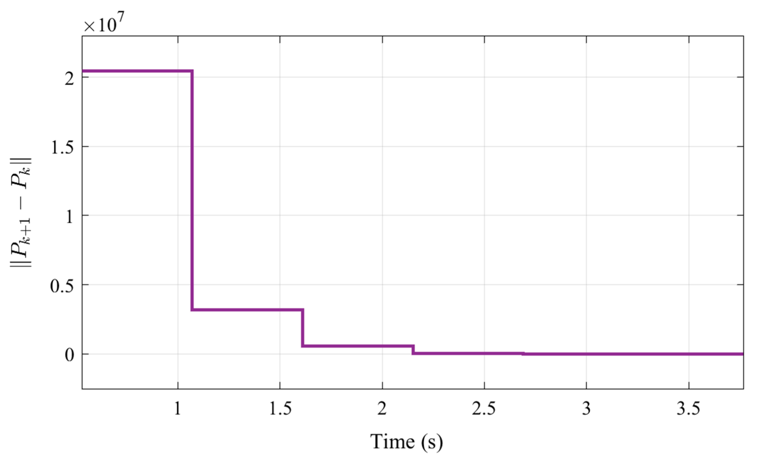
4.1. Online Learning and Optimization of Control Parameters

A rapid prototyping control (RPC) simulation platform, as shown in Figure 7, was established. The simulation hardware includes the MicroAutoBox II real-time system, Speedgoat baseline real-time target machines, and a host computer. The MicroAutoBox II is equipped with an IBM PPC 750GL processor (900 MHz), the host computer software is Matlab 2021b, and the Speedgoat baseline real-time target machines feature an Intel Celeron 2 GHz CPU with four cores. The host computer primarily runs Simulink interface programs, which transmit data to the Speedgoat prototype controller via UDP communication through a high-speed network port.

The MicroAutoBox II provides robust computational power, enabling real-time operation of complex half-car active suspension models. It calculates vehicle state information based on control signals sent from the Speedgoat target machine and transmits this information to the host computer. CAN communication can be configured using the Speedgoat and dSPACE driver libraries in Simulink, including settings for writing, reading, and status detection functions. The Speedgoat controller is used to execute the proposed online PI-RL algorithm, while MicroAutoBox II is employed to run the vehicle dynamics model and sensor model. A PC serves as the host computer for data recording and display. For the RPC system, the UDP is preferred due to its low-latency characteristics. Compared to the TCP, using the UDP reduces development and maintenance complexity and facilitates rapid deployment and debugging. Therefore, the UDP is chosen for host computer communication in this setup. In UDP communication, the host computer is connected to the host-link ports of the Speedgoat and MicroAutoBox II, and IP addresses are configured to ensure network communication. Communication between the controller and the vehicle dynamics model utilizes the CAN protocol, while data exchange between the controller, sensors, and host computer occurs via the UDP. The vehicle model parameters are listed in

Table 2. Vehicle model parameters.

Parameter	Value	Parameter	Value
M (kg)	500	$a\left(\mathrm{m}\right)$	1.25
J (kg·m2)	910	$b\left(\mathrm{m}\right)$	1.45
mt1 (kg)	30	$k_{s1}\left(\mathrm{N}/m\right)$	10,000
mt2 (kg)	40	$k_{s2}\left(\mathrm{N}/m\right)$	10,000
kt1 (N/m)	100,000	$u_{1\max }\left(\mathrm{N}\right)$	2000
kt2 (N/m)	100,000	$u_{2\max }\left(\mathrm{N}\right)$	2000
$b_{s1}\left(\mathrm{Ns}/m\right)$	1000	$b_{s2}\left(\mathrm{Ns}/m\right)$	1000
z1max (m)	0.1	kf (N/A)	40
z2max (m)	0.1	r (Ω)	25.3
$L_c\left(\mathrm{mH}\right)$	23.12	$N_c$	1262

, the inductance $L_c$ and number of turns $N_c$ of coil 2 are also given in Table 2, and the controller design parameters are selected as follows:

$$\begin{gathered} a=1,Q=\mathrm{diag}\left(\left[\begin{array}{cccccccc}10& 10& 10& 10& 200& 300& 10& 10\end{array}\right]\right), \\ R=0.0001\ast \mathrm{eye}(2),\delta =0.0001,\delta t=0.01 \end{gathered}$$

During the operation of the heuristic algorithm, the core step is to initially run the RL algorithm without considering the preset convergence rate, i.e., a = 0, allowing the initial parameter $K_0$ to be set to zero. Subsequently, the optimization results from the first step are used as the initial parameters for the second step. This approach avoids the complexity of parameter tuning, which is advantageous for high-dimensional systems. In the weight matrix $Q$, since our objective is to reduce vertical acceleration and pitch acceleration, $Q\left(5\right)$ and $Q\left(6\right)$ can be set relatively high. It is important to note that the PI algorithm will only be executed when $rank\left({\Theta }_k\right)=0.5n\left(n+1\right)+nm$ is satisfied; otherwise, sampling will continue until the condition is met. The heuristic algorithm proposed in this paper is not sensitive to exploratory noise, and for any Gaussian white noise, the basic optimization conditions can be met when the data length $l_k=0.5n\left(n+1\right)+nm$. Firstly, the initial step of running the heuristic algorithm is undertaken. During the learning process, the detection noise, as shown in Figure 8, is mainly generated by the linear motor, with its amplitude typically small and frequencies far from the system’s natural frequencies. Figure 9 displays the learning status signal, while Figure 10 illustrates the suspension’s state variables. Figure 11 depicts the variation of $‖P_{k+1}-P_k‖$, indicating the training completion at 3.77 s. As shown in Figure 11, when $‖P_{k+1}-P_k‖\le \delta$, the solution $P_k$ of the ARE converges to the optimal solution, i.e., at iteration step $k=5$. To validate the effectiveness of this method, directly solving the ARE (12) yields the ideal optimal solution. Figure 12 compares the actual control gain with the ideal value.

Furthermore, by incorporating the solved optimal control gains $K_0^{\ast }$ into the second step of the heuristic algorithm, choosing $\gamma =0.9$ yields the final optimal control gains considering the preset convergence performance, as depicted in Figure 13. Figure 14 illustrates the variation of suspension state variables during the learning process. In practice, values of $\gamma$ near 1 ensure the feasibility of the algorithm. Moreover, this method does not require the system’s model parameters; by introducing detection noise online, it can rapidly achieve the optimal control solution considering the preset convergence performance.

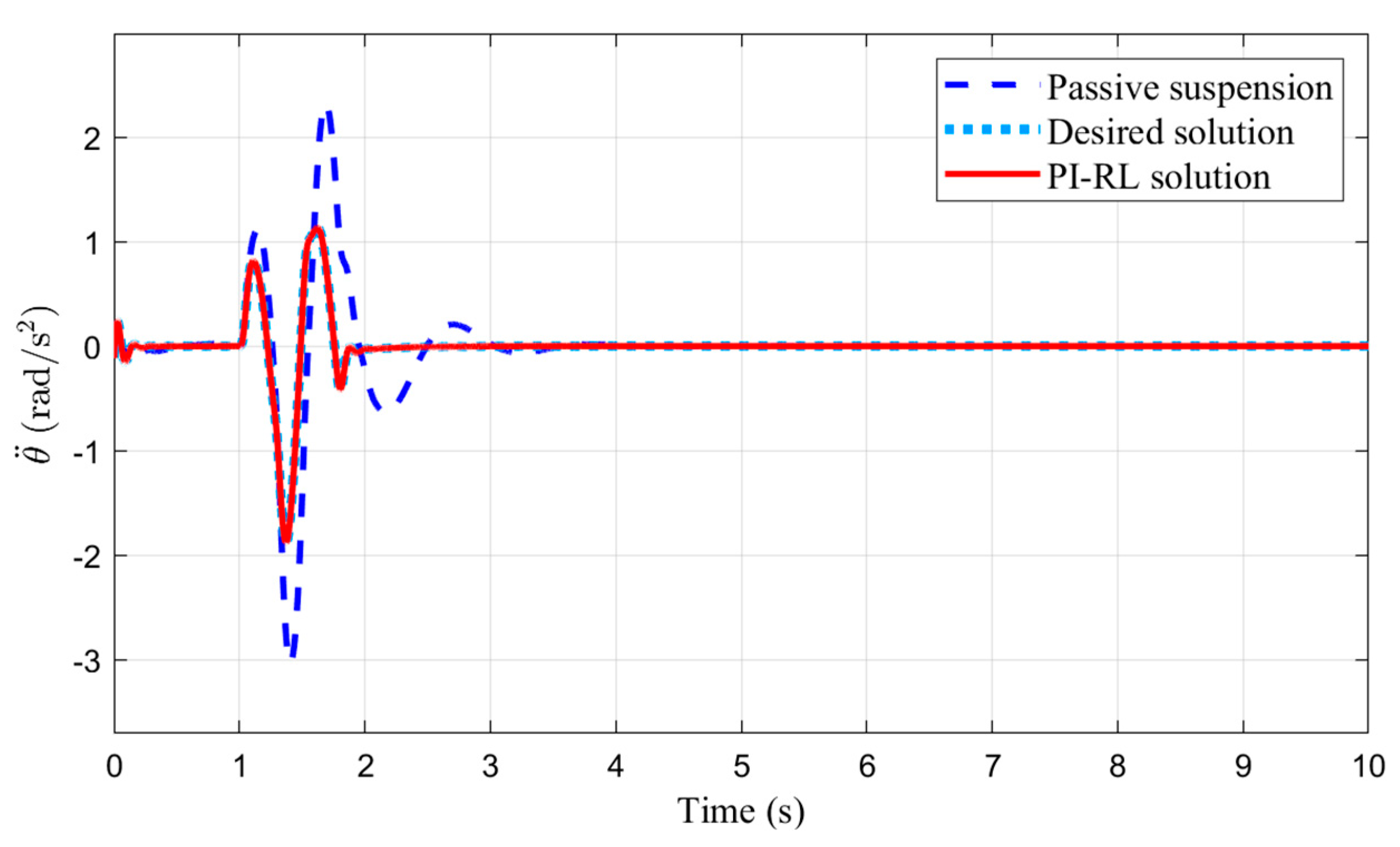
4.2. Control Implementation

To evaluate the performance of the proposed reinforcement learning vibration controller, road tests are conducted using bump road excitation (8). The test vehicle speed is set to 36 km/h, with a bump length of 5 m and a bump height of 0.1 m. The system’s initial state is set as a random number, and the simulation results are shown in Figure 15, Figure 16 and Figure 17. Figure 15 displays the vertical acceleration response curve of the vehicle. Figure 16 shows the pitch acceleration response curve, and Figure 17 presents the suspension output performance indicators.

The simulation compared the PI-RL solution with the ideal optimal control solution, demonstrating the effectiveness of the PI-RL algorithm proposed in the paper, as all performance metrics align with the ideal scenario.

Table 3. Suspension performance RMS value.

Method	${\ddot{\mathit{z}}}_{\mathit{c}}$$\left(\mathbf{m}/{\mathbf{s}}^2\right)$	$\ddot{\mathit{\theta }}$$\left(\mathbf{rad}/{\mathbf{s}}^2\right)$	${\mathit{P}}_{\mathit{r}\mathit{m}\mathit{s}1}$ (W)	${\mathit{P}}_{\mathit{r}\mathit{m}\mathit{s}2}$ (W)
Passive suspension	0.4531	0.4799	——	——
PI-RL (a = 0)	0.1818	0.2265	1133	1378
PI-RL (a = 0.3)	0.1858	0.2324	1087	1299
PI-RL (a = 0.6)	0.1914	0.2406	1034	1210
PI-RL (a = 1)	0.201	0.2551	958.6	1086
PI-RL (a = 1.2)	0.2067	0.2638	922.6	1026

compares the root mean square values of key suspension indicators under different preset convergence rates. It can be observed from the table that the preset convergence rate impacts motor thermal power. Increasing the preset convergence rate can reduce motor thermal power, although other indicators may slightly increase.

Figure 18 and Figure 19 show the power spectral density estimates of the vehicle’s vertical acceleration and pitch acceleration. The relationship between the normalized frequency $\omega$ and the temporal frequency $f$ is given by $f=\omega f_s/2\pi$, where $f_s$ is the sampling frequency, set at 1000 Hz in this study. From the figures, it is evident that effective attenuation is achieved in the 0–500 Hz range for both vertical and pitch acceleration, with particularly notable attenuation in the low-frequency range of 0–10 Hz (vibrations in the 4–8 Hz range have the most significant impact on human comfort). On highways and well-maintained urban roads, road excitation frequencies are typically below 3 Hz, whereas on rough roads or in rural areas, they are generally below 11 Hz [24]. Therefore, the PI-RL-based vibration control method is effective overall. Additionally, as noted in [15], reducing vertical and pitch acceleration in the 0.8–8 Hz range helps mitigate motion sickness.

5. Conclusions

This paper investigates a reinforcement learning-based vibration control method for electromagnetic active suspension systems with unknown model parameters. A half-vehicle active suspension control model is established. An online reinforcement learning algorithm based on PI is applied to design an optimal controller considering the preset convergence rate. A heuristic algorithm is proposed to ensure the feasibility of the solution. Rapid prototyping control simulations verify the feasibility of the proposed method, with a decrease in control energy consumption index as the preset convergence rate increases. Simulation tests on rough road surfaces indicate that all metrics of this method are significantly better than those of passive suspensions, with over 40% reduction in vertical and pitch accelerations. Frequency domain analysis demonstrates the effectiveness of this method within the low-frequency range of 0~10 Hz, which can satisfy the driving comfort requirements on most common road surfaces. Future research will further consider the nonlinear characteristics of the model and fault-tolerant control performance, as well as the coordinated control mechanism between active suspension and steering systems.

References

1. Yu, M.; Evangelou, S.A.; Dini, D. Advances in Active Suspension Systems for Road Vehicles. Engineering 2024, 33, 160–177. [Google Scholar] [CrossRef]
2. Zhao, W.; Gu, L. Adaptive PID Controller for Active Suspension Using Radial Basis Function Neural Networks. Actuators 2023, 12, 437. [Google Scholar] [CrossRef]
3. Ding, R.; Wang, R.; Meng, X.; Chen, L. Energy consumption sensitivity analysis and energy-reduction control of hybrid electromagnetic active suspension. Mech. Syst. Signal Process. 2019, 134, 106301. [Google Scholar] [CrossRef]
4. Su, X.; Yang, X.; Shi, P.; Wu, L. Fuzzy control of nonlinear electromagnetic suspension systems. Mechatronics 2014, 24, 328–335. [Google Scholar] [CrossRef]
5. Liu, L.; Li, X.; Liu, Y.-J.; Tong, S. Neural network based adaptive event trigger control for a class of electromagnetic suspension systems. Control. Eng. Pract. 2021, 106, 104675. [Google Scholar] [CrossRef]
6. Pang, H.; Wang, M.; Wang, L.; Luo, J. A composite vibration control strategy for active suspension system based on dynamic event triggering and long and short-term memory neural network. IEEE Trans. Transp. Electrif. 2023, 1. [Google Scholar] [CrossRef]
7. Wong, P.K.; Li, W.; Ma, X.; Yang, Z.; Wang, X.; Zhao, J. Adaptive event-triggered dynamic output feedback control for nonlinear active suspension systems based on interval type-2 fuzzy method. Mech. Syst. Signal Process. 2024, 212, 111280. [Google Scholar] [CrossRef]
8. Zhou, Z.; Zhang, M.; Liu, H.; Jing, X. Fixed-Time Safe-by-Design Control for Uncertain Active Vehicle Suspension Systems With Nonlinear Reference Dynamics. IEEE/ASME Trans. Mechatron. 2023, 1–12. [Google Scholar] [CrossRef]
9. Huang, T.; Wang, J.; Pan, H. Adaptive bioinspired preview suspension control with constrained velocity planning for autonomous vehicles. IEEE Trans. Intell. Veh. 2023, 8, 3925–3935. [Google Scholar] [CrossRef]
10. Zhang, Z.; Zhang, J.; Yin, H.; Zhang, B.; Jing, X. Bio-inspired structure reference model oriented robust full vehicle active suspension system control via constraint-following. Mech. Syst. Signal Process. 2022, 179, 109368. [Google Scholar] [CrossRef]
11. Qin, Z.C.; Xin, Y. Data-driven H∞ vibration control design and verification for an active suspension system with unknown pseudo-drift dynamics. Commun. Nonlinear Sci. Numer. Simul. 2023, 125, 107397. [Google Scholar] [CrossRef]
12. Liu, Z.; Si, Y.; Sun, W. Ride comfort oriented integrated design of preview active suspension control and longitudinal velocity planning. Mech. Syst. Signal Process. 2024, 208, 110992. [Google Scholar] [CrossRef]
13. Guo, X.; Zhang, J.; Sun, W. Robust saturated fault-tolerant control for active suspension system via partial measurement information. Mech. Syst. Signal Process. 2023, 191, 110116. [Google Scholar] [CrossRef]
14. Wang, W.; Liu, S.; Zhao, D.; Zhang, C. Approximation-free output feedback control for hydraulic active suspensions with prescribed performance. Nonlinear Dyn. 2023, 111, 21673–21689. [Google Scholar] [CrossRef]
15. Jeong, Y.; Yim, S. Design of active suspension controller for ride comfort enhancement and motion sickness mitigation. Machines 2024, 12, 254. [Google Scholar] [CrossRef]
16. Liu, L.; Sun, M.; Wang, R.; Zhu, C.; Zeng, Q. Finite-Time Neural Control of Stochastic Active Electromagnetic Suspension System With Actuator Failure. IEEE Trans. Intell. Veh. 2024, 1–12. [Google Scholar] [CrossRef]
17. Shaqarin, T.; Noack, B.R. Enhancing Mechanical Safety in Suspension Systems: Harnessing Control Lyapunov and Barrier Functions for Nonlinear Quarter Car Model via Quadratic Programs. Appl. Sci. 2024, 14, 3140. [Google Scholar] [CrossRef]
18. Afshar, K.K.; Korzeniowski, R.; Konieczny, J. Evaluation of Ride Performance of Active Inerter-Based Vehicle Suspension System with Parameter Uncertainties and Input Constraint via Robust H Control. Energies 2023, 16, 4099. [Google Scholar] [CrossRef]
19. Arumugam, K.; Chen, B.-S. Finite-time based fault-tolerant control for half-car active suspension system with cyber-attacks: A memory event-triggered approach. IEEE Trans. Veh. Technol. 2024, 1–13. [Google Scholar] [CrossRef]
20. Huang, T.; Wang, J.; Pan, H. Approximation-Free Prespecified Time Bionic Reliable Control for Vehicle Suspension. IEEE Trans. Autom. Sci. Eng. 2023, 1–11. [Google Scholar] [CrossRef]
21. Pan, H.; Zhang, C.; Sun, W. Fault-Tolerant Multiplayer Tracking Control for Autonomous Vehicle via Model-Free Adaptive Dynamic Programming. IEEE Trans. Reliab. 2022, 72, 1395–1406. [Google Scholar] [CrossRef]
22. Li, Q.; Chen, Z.; Song, H.; Dong, Y. Model Predictive Control for Speed-Dependent Active Suspension System with Road Preview Information. Sensors 2024, 24, 2255. [Google Scholar] [CrossRef] [PubMed]
23. Wang, G.; Li, K.; Liu, S.; Jing, H. Model-Free H∞ Output Feedback Control of Road Sensing in Vehicle Active Suspension Based on Reinforcement Learning. J. Dyn. Syst. Meas. Control 2023, 145, 061003. [Google Scholar] [CrossRef]
24. Kim, J.; Yim, S. Design of Static Output Feedback Suspension Controllers for Ride Comfort Improvement and Motion Sickness Reduction. Processes 2024, 12, 968. [Google Scholar] [CrossRef]
25. Li, P.; Lam, J.; Cheung, K.C. Multi-objective control for active vehicle suspension with wheelbase preview. J. Sound Vib. 2014, 333, 5269–5282. [Google Scholar] [CrossRef]
26. Jiang, Y.; Zhang, K.; Wu, J.; Zhang, C.; Xue, W.; Chai, T.; Lewis, F.L. H∞-based minimal energy adaptive control with preset convergence rate. IEEE Trans. Cybern. 2021, 52, 10078–10088. [Google Scholar] [CrossRef]
27. Jiang, Y.; Jiang, Z.-P. Computational adaptive optimal control for continuous-time linear systems with completely unknown dynamics. Automatica 2012, 48, 2699–2704. [Google Scholar] [CrossRef]
28. Esmaeili, J.S.; Akbari, A.; Farnam, A.; Azad, N.L.; Crevecoeur, G. Adaptive Neuro-Fuzzy Control of Active Vehicle Suspension Based on H2 and H∞ Synthesis. Machines 2023, 11, 1022. [Google Scholar] [CrossRef]
29. Dridi, I.; Hamza, A.; Ben Yahia, N. A new approach to controlling an active suspension system based on reinforcement learning. Adv. Mech. Eng. 2023, 15, 16878132231180480. [Google Scholar] [CrossRef]
30. Li, H.; Liu, D.; Wang, D. Integral reinforcement learning for linear continuous-time zero-sum games with completely unknown dynamics. IEEE Trans. Autom. Sci. Eng. 2014, 11, 706–714. [Google Scholar] [CrossRef]
31. Li, C.; Ding, J.; Lewis, F.L.; Chai, T. Model-free Q-learning for the tracking problem of linear discrete-time systems. IEEE Trans. Neural Netw. Learn. Syst. 2022, 35, 3191–3201. [Google Scholar] [CrossRef] [PubMed]
32. Valadbeigi, A.P.; Sedigh, A.K.; Lewis, F.L. H∞ Static Output-Feedback Control Design for Discrete-Time Systems Using Reinforcement Learning. IEEE Trans. Neural Netw. Learn. Syst. 2019, 31, 396–406. [Google Scholar] [CrossRef] [PubMed]
33. Yang, Y.; Wan, Y.; Zhu, J.; Lewis, F.L. H∞ tracking control for linear discrete-time systems: Model-free Q-learning designs. IEEE Control. Syst. Lett. 2020, 5, 175–180. [Google Scholar] [CrossRef]
34. Lian, B.; Donge, V.S.; Lewis, F.L.; Chai, T.; Davoudi, A. Data-driven inverse reinforcement learning control for linear multiplayer games. IEEE Trans. Neural Netw. Learn. Syst. 2022, 35, 2028–2041. [Google Scholar] [CrossRef] [PubMed]
35. Wang, D.; Gao, N.; Liu, D.; Li, J.; Lewis, F.L. Recent progress in reinforcement learning and adaptive dynamic programming for advanced control applications. IEEE/CAA J. Autom. Sin. 2023, 11, 18–36. [Google Scholar] [CrossRef]
36. Wei, W.; Li, Q.; Xu, F.; Zhang, X.; Jin, J.; Jin, J.; Sun, F. Research on an electromagnetic actuator for vibration suppression and energy regeneration. Actuators 2020, 9, 42. [Google Scholar] [CrossRef]
Figure 1. Structure of electromagnetic suspension.
Processes 12 01591 g001
Figure 2. Linear motor structure.
Processes 12 01591 g002
Figure 3. Modeling nomenclature of a linear motor.
Processes 12 01591 g003
Figure 4. Half-car active suspension model.
Processes 12 01591 g004
Figure 5. Equivalent state-space model.
Processes 12 01591 g005
Figure 6. PI-RL algorithm.
Processes 12 01591 g006
Figure 7. Rapid prototyping control simulation platform.
Processes 12 01591 g007
Figure 8. Exploration noise.
Processes 12 01591 g008
Figure 9. Learning status signal.
Processes 12 01591 g009
Figure 10. Suspension state variables ( a = 0 ).
Processes 12 01591 g010
Figure 11. P k + 1 P k .
Processes 12 01591 g011
Figure 12. PI-RL solution and ideal solution ( a = 0 ).
Processes 12 01591 g012
Figure 13. PI-RL solution and ideal solution ( a = 1 ).
Processes 12 01591 g013
Figure 14. Suspension state variables ( a = 1 ).
Processes 12 01591 g014
Figure 15. Vertical acceleration curve.
Processes 12 01591 g015
Figure 16. Pitch acceleration curve.
Processes 12 01591 g016
Figure 17. Suspension performance output Λ 2 .
Processes 12 01591 g017
Figure 18. Vertical acceleration power spectral density.
Processes 12 01591 g018
Figure 19. Pitch acceleration power spectral density.
Processes 12 01591 g019