Abstract
This paper presents a methodology for fault detection and isolation (FDI) in transient conditions using a multiway principal component analysis (MPCA) approach where practical data have been augmented with simulated data to conduct FDI when there are insufficient practical data. The motivation for using a heated two-tank system is due to the fact that it resembles a basic process in terms of controllable variables, noise, disturbances, and changes in operating points. Normal and faulty condition data of the practical heated two-tank system as well as a Simulink® model of the heated two-tank system were used. The MPCA technique has enhanced ability to detect and isolate faults in transient conditions compared to classic principal component analysis (PCA). MPCA, however, requires a vast amount of normal process transient conditions data to train the model to then enable meaningful fault detection and isolation. In this study, the practical normal transient conditions data are augmented with simulated normal transient conditions data to meet the requirement of a large amount of data. Utilising different datasets for the training of the MPCA model, the fault detection and isolation performance was evaluated with various metrics. This paper presents positive results towards the implementation of MPCA for fault detection in transient conditions.
1. Introduction
Data-driven approaches become particularly relevant when dealing with large volumes of accessible data. These methods transform historical data into a priori knowledge essential for diagnostic systems [1]. The widespread adoption of data-driven methods in industrial applications can be attributed to their minimal reliance on prior knowledge about the system and their relatively simpler modelling process in comparison to model-based approaches [2,3]. This approach is especially favoured in steady-state scenarios, where the complexities of developing specialised dynamic models for a system pose significant challenges [4]. The development of sensor technology has led to the incorporation of new variables into systems, generating more extensive datasets for process analysis [5]. While this increase in data is valuable, it also increases the system’s complexity, which poses challenges for fault detection. The statistical approach, particularly within history-based methods, has been extensively researched for its robust detection performance. Although its diagnostic capabilities may not be as advanced as some other approaches, in industrial applications, the emphasis is often on detection rather than diagnosis. Multivariate statistical techniques, such as PCA, are employed for the analysis of large datasets, as they reduce dimensionality while preserving essential information [4]. PCA is a linear dimension reduction technique for capturing dataset variance that allows for meaningful analysis of noise and correlation. Single-plot charts (e.g., and Q) are used to condense large datasets to allow for easy interpretation and trend identification. The reduced dimensionality enhances a system’s fault detection capabilities [6,7]. However, a limitation of PCA is that it is time-invariant, whereas most processes are time-varying, which requires recursive adjustment of the PCA model over time [4]. An adapted PCA approach called multiway principal component analysis (MPCA) is suggested to address these limitations [8,9]. MPCA rearranges a three-dimensional array of variables—time, batches, or transients—into a two-dimensional data matrix, which is subsequently analysed using PCA [10]. The MPCA technique is capable of accommodating nonlinear dynamics, enabling the detection of faults over time. However, it requires substantial amounts of data to perform effectively.
Several studies found in the literature face similar limitations in terms of process monitoring and have adapted the MPCA approach for enhanced process monitoring capabilities. Ng and Srinivasan [11] state that most process monitoring techniques are suitable for steady-state operation but inadequate for multiphase transient operations (or systems having different modes of operation) with complex dynamics. This is due to the fact that the statistics these techniques are developed on—normal distribution, stationary—are not valid in transient conditions. Ng and Srinivasan [11] developed an adjoined principal component analysis (AdPCA) methodology using overlapping PCA models to ensure smooth evolution of monitoring over different transient states. Grasso et al. [12] followed a sensor fusion methodology by combining a multivariate control chart approach combined with an MPCA for process monitoring using multi-channel profile data. Zhou et al. [13] developed sub-period division strategies combined with MPCA in order to detect anomalies in a wastewater treatment process. Their approach is based on similarities of the loading matrices between adjacent time slices. Liu et al. [14] also tackles a multiphase (multi-mode, having different transient conditions) batch monitoring problem using an automatic segmentation algorithm of dynamic and static models based on high-order slow feature analysis and MPCA. Another interesting study by Bregon et al. [15] evaluates the performance of their developed FDI method utilising simulated data and observers on a thermodynamic system comprising heated tank systems. Ruan et al. [16] developed a virtual bearing test bench in OpenModelica and then used it to generate simulation data for CNN training. The goal of this research was to examine whether the simulation data generated from the physics model can enhance CNN fault diagnosis when the trained CNN is applied directly to the experimental data.
This paper contributes by exploring the feasibility of fault detection and isolation in transient conditions using MPCA based on training data predominantly from simulation experiments. The investigation is performed on a practical heated two-tank system. Practical data from the system are available, as well as simulation data from a validated representative model of the system [17].
This paper is organised as follows: Section 2 provides an overview of the process used as an experimental platform. Section 3 reviews the MPCA approach in the context of FDI. The experiments to acquire the relevant data to train the MPCA model are motivated in Section 4. Section 5 presents the results and discussion, and finally, the paper is concluded in Section 6.
2. System Overview
Figure 1a shows the practical benchmark heated two-tank system used for this study. It is inexpensive and quick to build compared to a full-scale or prototype industrial system. The purpose of the system is not to replicate the precise physical properties of an industrial system but rather to emulate the same problems or faults that are typically encountered in a large-scale system [18]. The benchmark heated two-tank system is a multi-domain system with measured variables across physical domains such as temperature, flow rate, and liquid level. This system is representative of manufacturing industries such as petrochemical, paper making, and water treatment, requiring temperature, liquid level, and flow control [19]. The nonlinear behaviour of the integrated tank system, sensor noise, and closed-loop control give the fault detection technique validity, since these effects are also encountered in industrial systems.
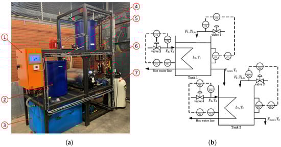
Figure 1.
Heated two-tank system. (a) Practical system. (b) P&ID diagram.
2.1. Benchmark Heated Two-Tank System
Figure 1b portrays the process and instrumentation diagram (P&ID) of the benchmark heated two-tank process with the external utilities shown in Figure 1a. Cold water from the reservoir is supplied to Tank 1 () and Tank 2 () at temperatures and , respectively. The level in Tank 1 () is controlled by regulating the flow via FC1. Similarly, the level in Tank 2 () is controlled by regulating the flow via FC2. The outlet of Tank 1 () flows into Tank 2, and the outlet of Tank 2 () flows back to the cold water reservoir.
Both Tank 1 and Tank 2 house heat exchangers in the form of copper coils to facilitate heat exchange to the content of the tanks. Hot water, , at temperature , is pumped through the coils of Tank 1. Similarly, hot water, , at temperature , is pumped through the coils of Tank 2. The flows and through the coils of Tank 1 and Tank 2 are regulated to control the temperatures and in Tank 1 and Tank 2, respectively.
The component descriptions of the heated two-tank process as shown in Figure 1a are summarised in Table 1. The process is controlled via a Siemens S7 Programmable Logic Controller (PLC) and supervised via a Human–Machine Interface (HMI). An Ethernet network connects the PLC to a standalone computer. Siemens’ Totally Integrated Automation Portal software is used to log process data at one-second intervals.

Table 1.
Process component descriptions.
The heated water from the process is returned to the cold water reservoir via a heat pump that cools down the water first. The hot water heater again heats and regulates the temperature of water streams and .
2.2. Simulated Data Compared to Practical
Various process variables are measured to obtain sufficient data of the process. Temperature, flow rate, and water level in the tanks are measured using different sensors and associated instrumentation. A breakdown of the measured variables can be seen in Table 2.
Table 2.
Measured variables—Tanks 1 and 2.
2.3. Model of Heated Two-Tank System
A Simulink® model of the heated two-tank system was initially created by Lindner and Auret [20,21,22]. Subsequently, the model was modified to incorporate process faults and to conform with the specifications of the laboratory setup.
2.4. Simulated Data Compared to Practical
To assess the simulation accuracy, the Normalised Root Mean Squared Error (NRMSE) metric was employed. The NRMSE ranges between 0 and 1 with lower values indicating better model fit [23]. The equation used to calculate the NRMSE is given by:
All the values are predominantly below 0.25 for most variables in Table 3, signifying a strong fit. The NRMSE values for the cold water flow rates in Tanks 1 and 2 are relatively higher compared to other variables but still remain below 1, indicating a reasonable level of accuracy.
Table 3.
NRMSE values of different variables.
To evaluate how the simulated data compare to the practical data, the transient response of the practical system is compared to that of the model across all measured variables. Figure 2 and Figure 3 illustrate how the practical data compared to simulated data for the level and temperature transients in Tank 1, respectively. The Simulink® model measured process variables, namely, the levels of the tanks and the temperatures in the tanks were altered to be representative of the actual measured process variables. For the levels of the tanks, the implementation translated to multiplying the level percentage with a uniform random number between 0.98 and 1.02. For the temperature, a pulse generator was used in the Simulink® model with the same resolution of the temperature sensor, i.e., 0.1 °C. The discrete nature of the temperature response is due to the resolution of the temperature sensors of 0.1 °C.
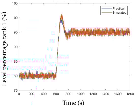
Figure 2.
Tank 1 level transient response, practical vs. simulated.
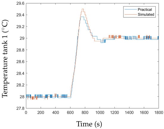
Figure 3.
Tank 1 temperature transient response, practical vs. simulated.
3. MPCA and FDI
PCA is widely used in chemical process monitoring [6]. PCA operates on the principle of linear dimensionality reduction, effectively reducing the dimensions of a multivariate dataset containing several interrelated variables. This technique involves the application of linear transformation to the data to generate new uncorrelated variables from the initially correlated variables within the dataset. In the presence of a transient in a process, the covariance matrix, utilised in constructing the PCA model, may undergo changes. This can result in the PCA monitoring process erroneously identifying normal transient behaviour as a fault [8]. Employing MPCA proves to be a viable solution to this issue. MPCA unfolds a three-way array into a two-dimensional data matrix that is subsequently mean-centred. This mean-centring process removes each mean trajectory in each column, effectively eliminating the main nonlinear and dynamic components in the data, allowing the application of PCA to datasets with transients. However, it is worth noting that MPCA demands a larger volume of data to achieve satisfactory performance. The initial step in applying the MPCA technique involves unfolding a three-way array of data under normal operation into a two-dimensional data matrix. In performing this, the process variable trajectories are contained in the two-dimensional data matrix. Following the creation of the two-dimensional data matrix, data conditioning is applied to enhance its compatibility with the technique. Subsequently, cross-validation is performed to determine the optimal number of principal components (PCs) for deployment in PCA. After using PCA to project the data into low-dimensional latent variable spaces, control limits can then be calculated for the squared predicted error (SPE) or Hotelling’s using normal data. The control limits are established to determine whether a new transient is normal or faulty.
3.1. Unfolding
In a transient, data are typically available for variables and samples . The data for the different transient runs of the same process can be categorised into intervals , if there are I transients. These available data can further be organised into a three-way array . The unfolding process is crucial in the MPCA technique and involves transforming the three-way array into a two-dimensional data matrix [8].
3.2. Data Preprocessing
Data preprocessing aims to enhance the performance of the MPCA technique and involves applying transformations and filters to the data. The following processes are included in the preprocessing stage: moving average, mean centring, and scaling to unit variance.
3.3. PCA
The first step in applying the PCA technique on the unfolded dataset with I rows and columns is to create a covariance matrix [6]:
where . Singular value decomposition can be performed on the covariance matrix:
Matrix contains the loading vectors, which are orthonormal column vectors providing the directions of maximum variability. The diagonal matrix contains the non-negative real eigenvalues in decreasing magnitude . The eigenvalues describe the magnitude of variance [6].
To capture the maximum variability of the dataset, the loading vectors corresponding to the largest eigenvalues are used. The loading matrix is obtained from the loading vectors corresponding to the first A eigenvalues or PCs. Loading matrix transforms data matrix into a reduced dimension space, which is the score matrix:
The projection of onto the score space is as follows:
The residual matrix can be obtained from the difference between and :
Lastly, the original data space can be reconstructed:
PCA power arises as it can provide a more parsimonious depiction of the covariance structure data. PCA offers an approximation of with just a few PCs.
3.4. Imputation
To enable online fault detection, where both past and current values are accessible but future transition values are not, two distinct methods can be considered. The first method involves the accurate approach of calculating and storing an MPCA model for each time step. However, this approach is encumbered by significant storage requirements, especially when dealing with large datasets. The second method opts for PCA without relying on MPCA. In this alternative, it assumes that the variables adhere to a multinormal distribution at each time interval. However, this method has its challenges. It necessitates the storage of a covariance matrix at each time interval, and this matrix becomes ill-conditioned due to the presence of highly correlated variables. Each approach presents trade-offs, and the choice between them depends on the specific considerations and constraints of the given scenario [10]. In a study by Garcia et al. [8], trimmed score regression (TSR) and known data regression using the principal component regression approach (KDR-PCR) yielded good results. Accordingly, the TSR method was used in this study to predict future values to be able to conduct online fault detection due to missing values. The KDR-PCR method can be used if the TSR method does not produce satisfactory results. The TSR approach enables the estimation of the score vector for computing missing values, facilitating the implementation of online monitoring. The TSR approach can be expressed by:
can be partitioned into
where the past and current values are and the unknown values are . The loading matrix can be partitioned into the following:
The estimated score vector is used to calculate the and SPE statistic in the next subsection.
3.5. Control Limits
Two multivariate control charts can be employed to monitor the system. The detection of a system fault is triggered if the values of the squared prediction error (SPE) and Hotelling’s statistic exceed the calculated fixed threshold [8]. To streamline both control charts, the upper control limit threshold can be set to a unitary value of 1, and then the statistics are normalised for the transients.
3.5.1. Hotelling’s
A fault is detected using the statistic when there is a variation in latent variables that is not accounted for by normal system variation. The statistic can be calculated as follows:
using the observation vector . To detect outliers, the threshold for the statistic is calculated using the following equation:
Considering I transients and A PCs, the critical value for significance level (expressed as ) is derived from the Fisher–Snedecor distribution with A and degrees of freedom, as indicated by Russel et al. [6]. These authors note that Hotelling’s statistic remains unaffected by smaller singular values and effectively characterises the normal behaviour of the process.
3.5.2. Square Prediction Error
The square prediction error (SPE) statistic gauges the cumulative variation in the residual space rather than measure individual loading vectors, ensuring that it remains robust even in the presence of smaller singular values and avoiding inaccuracies. The statistic is highly sensitive to inaccuracies in the projected space, as it measures the variation along the loading vectors [6]. In contrast, the SPE statistic is calculated at each specific instant k, providing the instantaneous perpendicular distance to the reduced space:
The value is calculated in the current measured vector at the time instant k, as:
with
where v is the variance and m is the mean required to calculate the upper limit of the SPE statistic using the chi-square distribution in the following equation [8]:
with
Using the SPE and statistics along with their respective upper limits, a fault can be detected when the calculated statistic exceeds the established upper limit. This implies that an unusual deviation from the normal process behaviour, beyond the acceptable threshold, has occurred.
3.6. Contribution Plot
Contribution plots can be used to isolate the fault. Abnormal deviation points in the transient can be used to derive a contribution plot [24]. The highest statistical point, whether or SPE, is selected to identify abnormal deviations over time, enabling the calculation of each variable’s contribution. The following equation is used to calculate the contribution plot for the statistic:
The following equation is used to calculate the contribution plot for the SPE statistic:
4. Experimental Design
This study involved both practical and simulation experiments. The experiments conducted on the practical system include normal and faulty system transients. A transient in this paper refers to a change in operating point by changing the setpoints for tank levels and tank temperatures in the system. Even though a fault can cause a transient, fault detection and isolation are evaluated during the transient caused by the change in operating setpoint. For faulty system transients, the faults are introduced at the exact instant that an operating setpoint change is introduced. The same procedure is followed for both the simulation and practical experiments to ensure uniformity in the results. MATLAB® was used as a simulation environment for data generation. Simulation experiments are relatively quick to conduct compared to practical experiments. The simulation model was validated with practical experiments [17]. The experimental design involves the specification of the different practical and simulation experiments to obtain the necessary data to evaluate the feasibility of applying MPCA-based training data from predominantly simulation experiments.
4.1. Normal Operation
In the practical experiments, the system is first brought to a steady state under normal operating conditions (NOC). Data collection occurs during the steady state for a duration of 500 s. Following this, a transient is introduced and data collected for a further 1200 s. The temperature of the cold reservoir is maintained at 24 °C using the heat pump for cooling, while the hot water reservoir is kept at 47 °C by means of the hot water heater.
Each transient involves identical changes in setpoint values for the temperatures and tank levels in Tank 1 and Tank 2. For the initial operating conditions, the temperature of Tank 1 is set at 27 °C and Tank 2 is set at 28 °C. These temperatures, close to the ambient temperature, ensure minimal heat exchange with the environment. Both tanks start with a level of 80% to prevent water spillage, particularly given that at levels below 80%, the water approaches the height of the agitator blades. The temperature setpoint for Tank 1 is adjusted from 27 °C to 28 °C and from 28 °C to 29 °C for Tank 2, maintaining a 1 °C difference due to the system’s dynamic temperature range. Larger temperature transients would result in impractically long settling times. The level setpoints are altered to 95% full, prompting the control system to adjust the flow of cold and hot water to attain the required temperature and tank level setpoint values. The change in temperatures and water levels represents the transient.
4.1.1. Practical Experiments
In total, 22 practical experiments were conducted, following the operational transient description outlined in Section 4.1 with some of the experiments incorporating emulated faults. The emulated faults exhibited distinct effects on various variables, and the magnitude of these faults also varied. The practical experiments that were run for the same transient are summarised in Table 4. The description column delineates the type of run, e.g., an NOC or a specific fault, while the fault implementation column further delineates with more specifics, e.g., fault size, as applicable. The blockage between Tanks 1 and 2 at 30% valve closure was conducted four times to evaluate the repeatability of the performance. The application column specifies whether the particular batch of transients was used for training or testing.
Table 4.
Practical experiments summarised.
Figure 4 illustrates the practical level in Tank 1 for both a normal transient (PNO1) and a transient under a stuck valve fault condition (PFS1). The fault and the transient are simultaneously introduced at time instant 600 s.
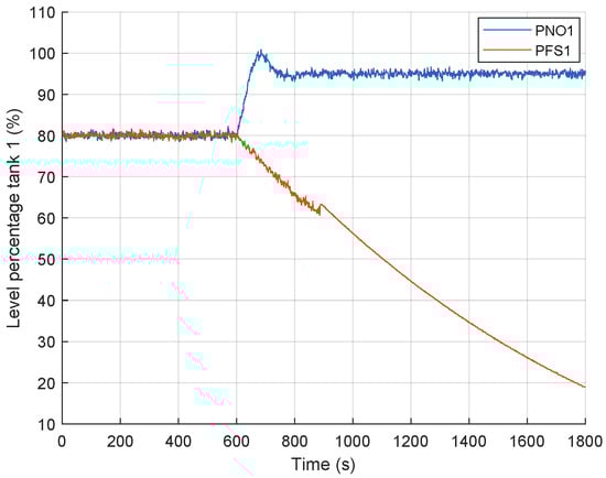
Figure 4.
Tank 1 practical level transient response, normal (PNO1) vs. stuck valve fault (PFS1).
4.1.2. Simulation Experiments
To run realistic NOC simulation experiments, it is crucial to measure and apply the typical changes that occur in the practical experiments. Two key variances between experimental runs were identified for this purpose, namely, offsets in measured variables and disturbance-associated noise. The variances are attributed to environmental effects such as ambient temperature and latent heat. The agitators furthermore induce fluctuations in water levels, resulting in disturbances. Additionally, noise generated by motors and measuring sensors contributes to the overall system noise. The noise and offset changes from practical signals are characterised and emulated in the simulation experiments. Realistic disturbances were uniquely introduced for each simulation experiment, by introducing white Gaussian noise with a unique seed value as well as unique random offsets in the data to account for environmental effects. The simulation experiments that were run for the same transient as described in Section 4.1 are summarised in Table 5. A total of 405 NOC simulation experiments were run and divided into 400 (SNO1 to SNO400) for model training and 5 (SNO401 to SNO405) for testing. Additionally, a faulty transient involving a blockage between the two tanks at the 30% closed valve position was simulated, denoted by unique IDs SFB31 to SFB34.
Table 5.
Simulation experiments summary.
4.1.3. Training and Testing
To evaluate the feasibility of applying MPCA, based on training data from predominantly simulation experiments, the strategy of combining the datasets needs to be carefully considered. The first consideration was to evaluate MPCA models with varying numbers of principal components (PCs), namely, 5, 10, 20, and 30. Then, two distinct classes of MPCA models were considered. One is where training is based purely on practical or purely on simulation experiments, hereafter referred to as the uncombined data class. The second class is where data from practical and simulation experiments are combined to form augmented training datasets, hereafter referred to as the combined data class.
For the uncombined data class, the training cases as illustrated in Table 6 are used. For each number of PCs, the model is either trained with data from 3 NOC practical experiments (PNOs) or data from a varying number of NOC simulation experiments (SNOs), namely, 5, 25, 50, 100, 200, or 400. The PM in Table 6 refers to the performance metric that will be associated with each training case.
Table 6.
Uncombined class training cases.
For the combined data class, data from the 400 NOC simulation experiments (SNO1–SNO400) were combined with the data from the 3 NOC practical experiments (PNO1–PNO3) to form various combinations for model training. For the combined data class, the training cases as illustrated in Table 7 are used. For each number of PCs, the model is trained with the following combinations of PNOs and SNOs designated as PNO + SNO: 3 + 2, 3 + 22, 3 + 47, 3 + 97, 3 + 197 or 3 + 397. The total of the combined data class equals the total for the uncombined data class. Similarly, the PM in Table 7 refers to the performance metric that will be associated with each training case.
Table 7.
Combined class training cases.
After training a model case, its performance is assessed using a fixed set of testing data comprising 5 NOC simulation experiments (SNO401–SNO405), 2 NOC practical experiments (PNO4–PNO5), 17 faulty system practical experiments (PFS1, PFS2, PFA1, PFA2, PFA12, PFL11–PFL13, PFL21–PFL23, PFB11, PFB21, PFB3–PFB34), and 4 faulty system simulation experiments (SFB31–SFB34).
The performance metrics considered in this study include the SPE-based false alarm rate (SFAR) and fault detection rate (SFDR) and the -based false alarm rate (TFAR) and fault detection rate (TFDR). It is important to note that the SFAR and TFAR performance metrics are based on fault or no fault classification per test experiment or transient; in this case, there are 7 NOC test transients in total, implying a resolution in the results. SFDR and TFDR performance metrics are similarly based on a fault or no fault classification per test experiment or transient; in this case, there are 21 faults in total, implying a resolution in the results.
5. Results and Discussion
The SFAR, SFDR, TFAR, and TFDR results for the uncombined data class are summarised in Table 8, Table 9, Table 10 and Table 11.
Table 8.
SFAR—uncombined class.
Table 9.
TFAR—uncombined class.
Table 10.
SFDR—uncombined class.
Table 11.
TFDR—uncombined class.
Table 8 indicates that as the number of simulation experiments included for training increases and the number of PCs decreases, the SFAR decreases until SNO = 50. Beyond SNO = 50, no further false alarms are observed. The elevated SFAR with a low number of SNOs is attributed to the control limit, as mentioned in [25]. With an increased number of SNOs, a control limit with lower false alarms can be established as the control limit relies on the variance and mean of the SNOs. The variance and mean of the SNOs are thus better characterised when a larger number are used. When robustness to false alarms increases, the sensitivity to fault detection decreases. In Table 10, it is evident that at a low number of PCs and a high number of SNOs (e.g., at 5 PCs and 400 SNOs), the SFDR is notably low.
Table 9 is obtained using the control chart. The control chart has fewer false alarms than the SPE, as seen in Table 8. Almost no false alarms are evident in Table 9. The control chart displays high robustness at a low number of SNOs and high number of PCs. The highest TFDR in Table 11 is 71% for any combination of data and PCs. With a high number of SNOs and a low number of PCs, the best performance is achieved as reported in Table 11.
The SFAR, SFDR, TFAR, and TFDR results for the combined data class are summarised in Table 12, Table 13, Table 14 and Table 15. The combined data class results reveal that comparable FDI performance is achieved with less training data, compared to the uncombined data class results. Table 8 reveals an SFAR of 14% at 10 PCs and 25 SNOs for the uncombined data class, whereas Table 12 reveals a 0% SFAR for the corresponding 10 PCs and PNO + SNO = 3 + 22 case.
Table 12.
SFAR—combined class.
Table 13.
TFAR—combined class.
Table 14.
SFDR—combined class.
Table 15.
TFDR—combined class.
Table 15 reveals that, for the combined data class, a lower (PNO + SNO) total is required to achieve the same fault detection rate (FDR) when compared to the corresponding uncombined data class case in Table 11. Interestingly, there is no notable difference in performance when using combined data for the control chart. In both cases, the maximum FDR remains at 71% with a 0% false alarm rate (FAR).
The results reveal comparable FDI performance for the combined data and uncombined data classes. While both classes achieved a maximum FDR of 81% at 0% FAR, the amount of training data required for each to achieve these comparable results differed. Next, an overall performance metric was defined to compare the different training classes and cases:
The SFAR and the TFAR are each subtracted from 100% to obtain the performance relative to 100%. The OVP then simply represents the average of the four performance measures. The OVP results for the uncombined data and combined data classes are given in Table 16 and Table 17, respectively, and indicate that the best performance is observed for the 20 PCs and 100 experiments cases, as well as the 30 PCs and 200 experiments cases.
Table 16.
Overall performance metric for uncombined class.
Table 17.
Overall performance metric for combined class.
For transient monitoring, a 30 PCs MPCA model was trained using data from 200 experiments from the uncombined data (200 SNOs) and combined data (PNO + SNO = 3 + 197) classes.
The transient monitoring performance metrics reported are the time-based FAR and FDR for each testing experiment over the complete transient interval as portrayed in Table 18 and Table 19, respectively. The FAR results are based on test data from two NOC practical experiments (PNO1 and PNO1) and five NOC simulation experiments (SNO401–SNO405). In Table 18, the FAR percentages are generally low and appear normal, except for the experiment PNO1 when using the control chart. The combined data class show a 14% and 33% TFAR. This discrepancy might be attributed to environmental effects during the experiment as it is repeated multiple times, creating an impression of a fault.
Table 18.
Transient monitoring FAR result with a 30 PCs model and 200 training experiments.
Table 19.
Transient monitoring FDR result with a 30 PCs model and 200 training experiments.
The FDR results are based on test data from 21 faulty system experiments. From Table 19, the FDR performance differences between the various datasets used are minimal, regardless of the control chart employed. Detection rates approaching or reaching 100% were observed for faults involving stuck valves and agitator issues. However, faults PFL11, PFL12, PFL21, PFB11, and PFB12 exhibited detection rates lower than 50% across all metrics. Notably, fault PFL13 demonstrated a high detection rate using the SPE control chart but a low detection rate with the control chart.
Figure 5 and Figure 6, respectively, show an example of the normalised SPE statistic and the normalised statistic for a leakage fault. The results are normalised with respect to the upper control limit. The time the fault is introduced coincides with the time the transient is introduced.
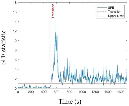
Figure 5.
SPE statictic for a Tank 1 leakage fault (30% valve open).
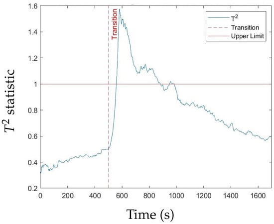
Figure 6.
statistic for a Tank 1 leakage fault (30% valve open).
The isolation of faults is performed by determining the variables with the greatest contribution to the SPE or statistic when a fault has been detected. In this system, eight variables are used. The contribution of each variable is represented as a percentage of the total contribution by all variables. Figure 7 and Figure 8 show the contributions of the different variables for the leakage fault in Tank 2 using the SPE and statistic, respectively. The level and flow of cold water into Tank 2 contributed the most to the leakage fault in Tank 2. All detected faults, except for the blockage at 30% valve closure, could be successfully isolated. In the case of the blockage at 30%, no common variable could be pinpointed, except for the flow rate of cold water into Tank 2.
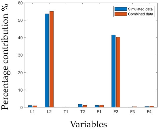
Figure 7.
SPE contribution plot of leakage fault in Tank 2.
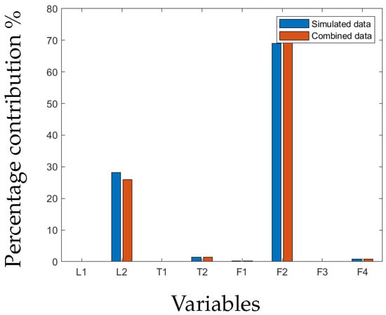
Figure 8.
contribution plot of leakage fault in Tank 2.
6. Conclusions
The performance of the MPCA approach was quantified through an overall performance metric. In this paper, the augmentation of practical data with simulated data to evaluate the performance of the MPCA method was explored. The methodology presented provides insight with respect to the efficacy of MPCA for FDI applied to the benchmark heated two-tank system. A promising result is that the MPCA model trained on the validated simulated model data showed good performance by detecting faults from experimental data. The leakage fault at the 10% open valve of Tank 1 or 2 and the blockage fault at 10% valve closure could not be detected. All detected faults, except for the blockage at 30% valve closure, could be successfully isolated. In the case of the blockage at 30%, no common variable could be pinpointed, except for the flow rate of cold water into Tank 2. The results of the paper contribute by exploring the augmentation of practical data with simulated data to improve the performance of the MPCA method.
Future work is warranted in ensuring a more even distribution of data across different fault types for both simulated and practical data. Uneven distributions may lead to biased models which can reduce fault detection and isolation performance.
Author Contributions
Conceptualization, G.v.S.; Software, M.C.D.; Investigation, W.M.K.v.N.; Writing—original draft, M.C.D.; Writing—review & editing, G.v.S. and K.R.U.; Supervision, G.v.S., Kenneth R. Uren and W.M.K.v.N. All authors have read and agreed to the published version of the manuscript.
Funding
This work is based on research supported by the SASOL-NRF research grant (grant number: 138606).
Data Availability Statement
Datasets and software related to this paper can be found on https://figshare.com.
Acknowledgments
Opinions expressed and conclusions reached are those of the authors and are not necessarily to be attributed to SASOL or the NRF.
Conflicts of Interest
The authors declare that they have no known competing financial interests or personal relationships that could have appeared to influence the work reported in this paper.
References
- Melo, A.; Câmara, M.M.; Pinto, J.C. Data-Driven Process Monitoring and Fault Diagnosis: A Comprehensive Survey. Processes 2024, 12, 251. [Google Scholar] [CrossRef]
- Reis, M.S.; Gins, G. Industrial process monitoring in the big data/industry 4.0 era: From detection, to diagnosis, to prognosis. Processes 2017, 5, 35. [Google Scholar] [CrossRef]
- Reis, M.S.; Gao, F. Special Issue “Advanced Process Monitoring for Industry 4.0”. Processes 2021, 9, 1432. [Google Scholar] [CrossRef]
- Venkatasubramanian, V.; Rengaswamy, R.; Kavuri, S.N.; Yin, K. A review of process fault detection and diagnosis: Part III: Process history based methods. Comput. Chem. Eng. 2003, 27, 327–346. [Google Scholar] [CrossRef]
- Yu, Y.; Peng, M.-J.; Wang, H.; Ma, Z.-G.; Li, W. Improved PCA model for multiple fault detection, isolation and reconstruction of sensors in nuclear power plant. Ann. Nucl. Energy 2020, 148, 107662. [Google Scholar] [CrossRef]
- Russel, E.; Chiang, L.H.; Braatz, R.D. Data-Driven Methods for Fault Detection and Diagnosis in Chemical Processes; Springer: London, UK, 2000; pp. 45–52. [Google Scholar] [CrossRef]
- Severson, K.; Molaro, M.; Braatz, R. Principal Component Analysis of Process Datasets with Missing Values. Processes 2017, 5, 38. [Google Scholar] [CrossRef]
- Garcia-Alvarez, D.; Fuente, M.J.; Sainz, G.I. Fault detection and isolation in transient states using principal component analysis. J. Process Control. 2012, 22, 551–563. [Google Scholar] [CrossRef]
- Park, Y.J.; Fan, S.K.S.; Hsu, C.Y. A Review on Fault Detection and Process Diagnostics in Industrial Processes. Processes 2020, 8, 1123. [Google Scholar] [CrossRef]
- Nomikos, P.; MacGregor, J.F. Multivariate SPC charts for monitoring batch processes. Technometrics 1995, 37, 41–59. [Google Scholar] [CrossRef]
- Ng, Y.S.; Srinivasan, R. An adjoined multi-model approach for monitoring batch and transient operations. Comput. Chem. Eng. 2009, 33, 887–902. [Google Scholar] [CrossRef]
- Grasso, M.; Colosimo, B.M.; Pacella, M. Profile monitoring via sensor fusion: The use of PCA methods for multi-channel data. Int. J. Prod. Res. 2014, 52, 6110–6135. [Google Scholar] [CrossRef]
- Zhou, J.; Huang, F.; Shen, W.; Liu, Z.; Corriou, J.P.; Seferlis, P. Sub-period division strategies combined with multiway principle component analysis for fault diagnosis on sequence batch reactor of wastewater treatment process in paper mill. Process Saf. Environ. Prot. 2021, 146, 9–19. [Google Scholar] [CrossRef]
- Liu, J.; Chen, P.H.; Chen, J. Automatic segmentation of dynamic and static models based on high order slow feature analysis and principal component analysis for multiphase batch monitoring. Expert Syst. Appl. 2024, 248, 123271. [Google Scholar] [CrossRef]
- Bregon, A.; Alonso-Gonzalez, C.J.; Pulido, B. Integration of Simulation and State Observers for Online Fault Detection of Nonlinear Continuous Systems. IEEE Trans. Syst. Man Cybern. Syst. 2014, 44, 1553–1568. [Google Scholar] [CrossRef]
- Ruan, D.; Chen, Y.; Gühmann, C.; Yan, J.; Li, Z. Dynamics Modeling of Bearing with Defect in Modelica and Application in Direct Transfer Learning from Simulation to Test Bench for Bearing Fault Diagnosis. Electronics 2022, 11, 622. [Google Scholar] [CrossRef]
- Wolmarans, W. A Comparison of PCA-and Energy-Based Fault Detection and Isolation in a Physical Heated Twotank Process. Master’s Thesis, North-West University, Potchefstroom, South Africa, 2022. [Google Scholar]
- Smith, R.S.; Doyle, J. Two tank experiment: A benchmark control problem. In Proceedings of the 1988 American Control Conference, Atlanta, GA, USA, 15–17 June 1988; Institute of Electrical and Electronics Engineers (IEEE): Piscataway, NJ, USA, 1988; Volume 88, pp. 2026–2031. [Google Scholar] [CrossRef]
- Adil, M.; Abid, M.; Khan, A.Q.; Mustafa, G. Comparison of PCA and FDA for monitoring of coupled liquid tank system. In Proceedings of the 2016 13th International Bhurban Conference on Applied Sciences and Technology, IBCAST 2016, Islamabad, Pakistan, 12–16 January 2016; pp. 225–230. [Google Scholar] [CrossRef]
- Lindner, B.S. Exploiting Process Topology for Optimal Process Monitoring. Master’s Thesis, Stellenbosch University, Stellenbosch, South Africa, 2014. [Google Scholar]
- Lindner, B.S.; Auret, L. Data-driven fault detection with process topology for fault identification. IFAC Proc. Vol. 2014, 47, 8903–8908. [Google Scholar] [CrossRef]
- Lindner, B.; Auret, L.; Bauer, M.; Groenewald, J.W. Comparative analysis of Granger causality and transfer entropy to present a decision flow for the application of oscillation diagnosis. J. Process Control 2019, 79, 72–84. [Google Scholar] [CrossRef]
- Thodda, G.; Madhavan, V.R.; Thangavelu, L. Predictive Modelling and Optimization of Performance and Emissions of Acetylene Fuelled CI Engine Using ANN and RSM. Energy Sources Part A Recovery Util. Environ. Eff. 2020, 45, 3544–3562. [Google Scholar] [CrossRef]
- Ferrer, A. Multivariate Statistical Process Control Based on Principal Component Analysis (MSPC-PCA): Some Reflections and a Case Study in an Autobody Assembly Process. Qual. Eng. 2007, 19, 311–325. [Google Scholar] [CrossRef]
- Kim, Y.I. Multivariate SPC for Batch Processes; The University of Alabama: Tuscaloosa, AL, USA, 2006. [Google Scholar]
Disclaimer/Publisher’s Note: The statements, opinions and data contained in all publications are solely those of the individual author(s) and contributor(s) and not of MDPI and/or the editor(s). MDPI and/or the editor(s) disclaim responsibility for any injury to people or property resulting from any ideas, methods, instructions or products referred to in the content. |
© 2024 by the authors. Licensee MDPI, Basel, Switzerland. This article is an open access article distributed under the terms and conditions of the Creative Commons Attribution (CC BY) license (https://creativecommons.org/licenses/by/4.0/).