A Coupling Model of Gas–Water Two-Phase Productivity for Multilateral Horizontal Wells in a Multilayer Gas Reservoir

Abstract

A series of complex horizontal wells have been implemented in challenging gas reservoirs. Multilateral horizontal well technology can be used in multilayer gas reservoirs, facilitating the expansion of the gas drainage area and enhancing productivity. Accurate productivity calculations for multilateral wells in multilayer reservoirs are essential for effective reservoir development. However, there have been few studies in this area. This paper introduces a coupling model for calculating the gas–water two-phase productivity of multilateral wells in multilayer reservoirs, based on the principles of conformal transformation and superposition of potential functions. The accuracy of the model is validated by obtaining the distribution of flow along the horizontal wellbore through numerical simulation cases. The results from the field case and sensitivity analysis indicate that the pressure difference increases nonlinearly from the toe to the heel, and the productivity of multilateral wells decreases as the gas–water ratio increases. The method proposed in this paper is applicable for calculating the productivity of multilateral wells in multilayer reservoirs.

1. Introduction

Nowadays, with the improvement of drilling and completion technology, multilateral wells are widely used in complex reservoirs [1,2,3]. Compared with vertical wells, multilateral wells can expand the drainage area, enabling a lower drawdown and facilitating the recovery of more oil and gas [4,5]. Therefore, multilateral wells are widely used in multilayered reservoirs, fractured reservoirs, and those with bottom water.

Many attempts have been made to characterize the productivity of horizontal wells, leading to the development of several models. For example, in 1988, Joshi considered the two endpoints of a horizontal well as the focal points of the drainage ellipse and treated the two-dimensional seepage zones in the x-y and y-z planes, as shown in Figure 1 [6]. In 1989, Babu and Odeh proposed a physical model for box reservoirs and developed a model for horizontal well capacity in the proposed steady state [7]. Kong et al. proposed a transient pressure response solution for multilateral horizontal wells, but it is difficult to calculate and apply [8]. Raghavan and Ambastha proposed a model for assessing the productivity of the horizontal well. However, their model did not account for interference between branches [9]. Wu et al. proposed a productivity equation for multi-branch horizontal wells in three-dimensional anisotropic reservoirs, but this analytical model did not consider the two-phase flow or the pressure drop in the wellbore [10]. Meng et al. proposed a semi-analytical model to evaluate the productivity of slanted wells, but the model did not take into account the variable mass flow in the wellbore [11]. There are also some studies which evaluated the pressure and productivity of fishbone wells [12,13,14].

However, most past analytical works on horizontal well productivity either assumed uniform flow throughout the wellbore or ignored the pressure drop along the wellbore. Such assumptions are not practical in many cases, especially in long horizontal wells. Therefore, some researchers have attempted to combine reservoir inflow and wellbore flow to predict horizontal well productivity. Overall, horizontal well capacity prediction models can be categorized into three types: analytical, semi-analytical, and numerical models.

Analytical models are widely accepted because they are quite convenient to use. Borisov proposed a productivity model for horizontal wells under a steady state. The boundary of the model is elliptical and ignores the formation damage caused by drilling and completion [15]. The analytical model has more assumptions and is far from the actual situation, and thus its use is limited. Giger et al. put forward an equation for the horizontal well in the center of the horizontal and vertical planes of the drainage body, but there is no derivation process in it [16]. However, the analytical model cannot accurately predict productivity because analytical models ignore the pressure drop of wellbores, potentially leading to an overestimation of productivity.

The semianalytical method involves iteratively calculating the productivity by coupling the reservoir seepage model with the flow characteristics in the wellbore. Many researchers have studied the semi-analytical model of productivity [17,18,19,20]. Penmatcha and Aziz developed a coupling model using a three-dimensional framework to calculate productivity [21]. Adesina et al. introduced an enhanced model which accounts for pressure drops because of acceleration [22]. Yan et al. studied the influence of dynamic non-equilibrium conditions on capillary pressure–saturation relationships under different pressure boundary conditions through numerical simulation and experimental methods, and they summarized the application of transient two-phase flow in porous media in geotechnical engineering [23,24,25]. The results showed that inertia is quite important for transient two-phase flow in porous media under dynamic non-equilibrium conditions. Therefore, the acceleration pressure drop and friction pressure drop should be considered in the horizontal well’s pressure drop, which makes the model more accurate. The semi-analytical model has higher accuracy than analytical models and is more effectively applied to field examples. For low permeability formation or natural fracture formation, some studies showed that the stress sensitivity of permeability cannot be ignored [26,27,28,29,30,31,32,33,34,35]. However, the current research on permeability stress sensitivity mainly focuses on the vertical well, with relatively less attention given to multilateral horizontal wells.

The numerical model can consider wellbore dynamics. Numerical models are used for detailed analysis of the long-term performance of wells, but it is necessary to describe the reservoir properties and big data in detail. Therefore, the numerical model cannot be used for rapid screening studies [36,37,38,39,40]. These models may not be all that convenient for petroleum engineers to use.

From the above literature review, there is an extremely limited amount of publications discussing the method of productivity for multilateral horizontal wells in multilayer gas reservoirs. In this paper, the authors propose a semianalytical model developed by coupling the reservoir inflow with the wellbore flow. The model is based on the principle of conformal transformation and superposition of potential functions, and the wellbore flow model used incorporates the accelerated pressure drop as well as the friction pressure drop. This model provides a convenient approach for calculating the productivity of multilateral wells in multilayer gas reservoirs.

2. Methodology

2.1. Basic Assumptions

In the y-z sections of the horizontal well, the top boundary is sealed, while the bottom boundary pressure is constant at p_i, as shown in Figure 2. The model is based on the following assumptions:

(1)

The gas reservoir is horizontal with a uniform reservoir thickness h, and it has a uniform initial pressure p_i;

(2)

The effects of gravity and capillary force are neglected;

(3)

The water flows steadily with a constant density and viscosity;

(4)

Considering two-phase steady state flow, the production process is isothermal and controlled by Darcy’s law;

(5)

The properties of the gas and reservoir are isotropic and homogeneous.

2.2. Coupling Modeling for Productivity of Horizontal Wells

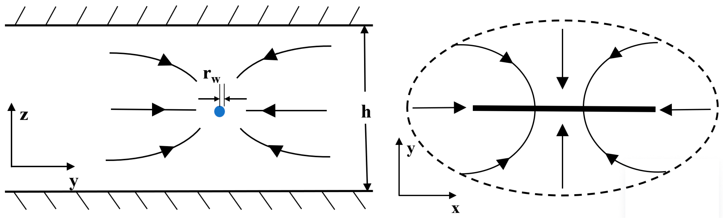
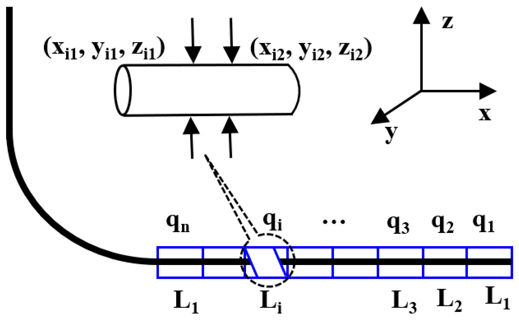
2.2.1. Reservoir Inflow Model

The horizontal wellbore is segmented into several microsegments. The length of the ith (i = 1, 2, 3, …, N) lateral is L_i, as shown in Figure 3, while (x_i1, y_i1, z_i1) and (x_i2, y_i2, z_i2) are the coordinates of the two endpoints of the ith lateral.

The potential function of a point sink is [37]

$$\varphi =-{\displaystyle \frac{q}{4\pi r}}+C$$

(1)

There exists any point M (x, y, z) within the infinite reservoir. Then, the potential of a horizontal microsegment i at point M is [41]

$${\varphi }_i\left(x,y,z\right)=-{\displaystyle \frac{q_i}{4\pi L_i}}\ln {\displaystyle \frac{R+L_i}{R-L_i}}+C$$

(2)

where

$$R=r_1+r_2=\sqrt{{\left(x_{i1}-x\right)}^2+y^2+{\left(z_{i1}-z\right)}^2}+\sqrt{{\left(x_{i2}-x\right)}^2+y^2+{\left(z_{i2}-z\right)}^2}$$

(3)

Based on the mirror image reflection law, the well in the reservoir with the top boundary seals and bottom water in the y-z section can be reflected as wells that line up in infinite space with two sinks and two sources. The coordinates of the two types of production wells are (x_i1, y_i1, 2h + 4nh − z_i1) and (x_i1, y_i1, 4nh + z_i1), while the coordinates of the two types of injection wells are (x_i1, y_i1, 2h + 4nh + z_i1) and (x_i1, y_i1, 4nh − z_i1), where n = 0, ±1, ±2, ±3, …

During the production of the ith micro-segment of a horizontal well, the potential generated at any point within the reservoir is [42]

$${\varphi }_i\left(x,y,z\right)=-{\displaystyle \frac{q_i}{4\pi L_i}}\left\{\sum _{n=\infty }^{+\infty }\left[\begin{array}{l}{\xi }_i\left(4nh+z_w,x,y,z\right)+{\xi }_i\left(4nh+2h-z_w,x,y,z\right)\\ -{\xi }_i\left(4nh-z_w,x,y,z\right)-{\xi }_i\left(4nh-2h+z_w,x,y,z\right)\end{array}\right]\right\}$$

(4)

where

$${\xi }_i\left({\zeta }_i,x,y,z\right)=\ln {\displaystyle \frac{R_N+L_i}{R_N-L_i}}$$

(5)

$$R_N=\sqrt{{\left(x-x_{i1}\right)}^2+y^2+{\left(z-{\zeta }_i\right)}^2}+\sqrt{{\left(x-x_{i2}\right)}^2+y^2+{\left(z-{\zeta }_i\right)}^2}$$

(6)

The potential distribution of infinite reservoirs generated by horizontal wells can be obtained using Equation (4):

$$\varphi \left(x,y,z\right)={\displaystyle \sum _{i=1}^n{\varphi }_i\left(x,y,z\right)}+C^{\prime }=-{\displaystyle \sum _{i=1}^n\frac{q_{gi}}{4\pi }{\phi }_i}+C^{\prime }$$

(7)

where

$${\phi }_i={\displaystyle \frac{1}{L_i}}\left\{\sum _{n=\infty }^{+\infty }\left[\begin{array}{l}{\xi }_i\left(4nh+z_w,x,y,z\right)+{\xi }_i\left(4nh+2h-z_w,x,y,z\right)\\ -{\xi }_i\left(4nh-z_w,x,y,z\right)-{\xi }_i\left(4nh-2h+z_w,x,y,z\right)\end{array}\right]\right\}$$

(8)

For two-phase seepage, the equations of motion can be described as follows [42]:

$${\displaystyle \frac{\mathrm{d}p}{\mathrm{d}r}}={\displaystyle \frac{{\mu }_g}{K·K_{\mathrm{rg}}}}{v}_g$$

(9)

$${\displaystyle \frac{\mathrm{d}p}{\mathrm{d}r}}={\displaystyle \frac{{\mu }_w}{K·K_{\mathrm{rw}}}}{v}_w$$

(10)

The law followed by the conservation of mass is expressed as follows:

$$Q_m=q_m{\rho }_m=q_g{\rho }_g+q_w{\rho }_w=q_{gsc}{\rho }_{gsc}+q_{wsc}{\rho }_{wsc}$$

(11)

By combining Equations (3)–(9), the reservoir seepage model for an infinite reservoir is established [42]:

$${\displaystyle {\int }_p^{p_{\mathrm{i}}}\left(\frac{K_{\mathrm{rg}}{\rho }_{\mathrm{g}}}{{\mu }_{\mathrm{g}}}+\frac{K_{\mathrm{rw}}{\rho }_{\mathrm{w}}}{{\mu }_{\mathrm{w}}}\right)}\mathrm{d}p={\displaystyle \frac{1}{0.0864}}{\displaystyle \frac{q_{gsc}({\rho }_{gsc}+R_{wg}{\rho }_{wsc})}{4\pi k_{\mathfrak{i}}}}{\phi }_i$$

(12)

where

$$R_{\mathrm{wg}}={\displaystyle \frac{q_{\mathrm{wsc}}}{q_{\mathrm{gsc}}}}$$

(13)

The two-phase generalized pseudo-pressure can be expressed as follows [42]:

$$m(p)={\displaystyle {\int }_p^{p_{\mathrm{i}}}\left(\frac{K_{\mathrm{rg}}{\rho }_{\mathrm{g}}}{{\mu }_{\mathrm{g}}}+\frac{K_{\mathrm{rw}}{\rho }_{\mathrm{w}}}{{\mu }_{\mathrm{w}}}\right)}\mathrm{d}p$$

(14)

Then, Equation (12) is simplified to

$$m(p)={\displaystyle \frac{1}{0.0864}}{\displaystyle \frac{q_{gsc}({\rho }_{gsc}+R_{wg}{\rho }_{wsc})}{4\pi k_{\mathfrak{i}}}}{\phi }_i$$

(15)

where ρ_g is the underground gas phase density in g/cm³; μ_g is the underground gas phase viscosity in mPa·s; ρ_w is the underground water phase density in g/cm³; μ_w is the underground water phase viscosity in mPa·s; and ρ_gsc and ρ_wsc refer to the gas density and water density under standard conditions in g/cm³, respectively.

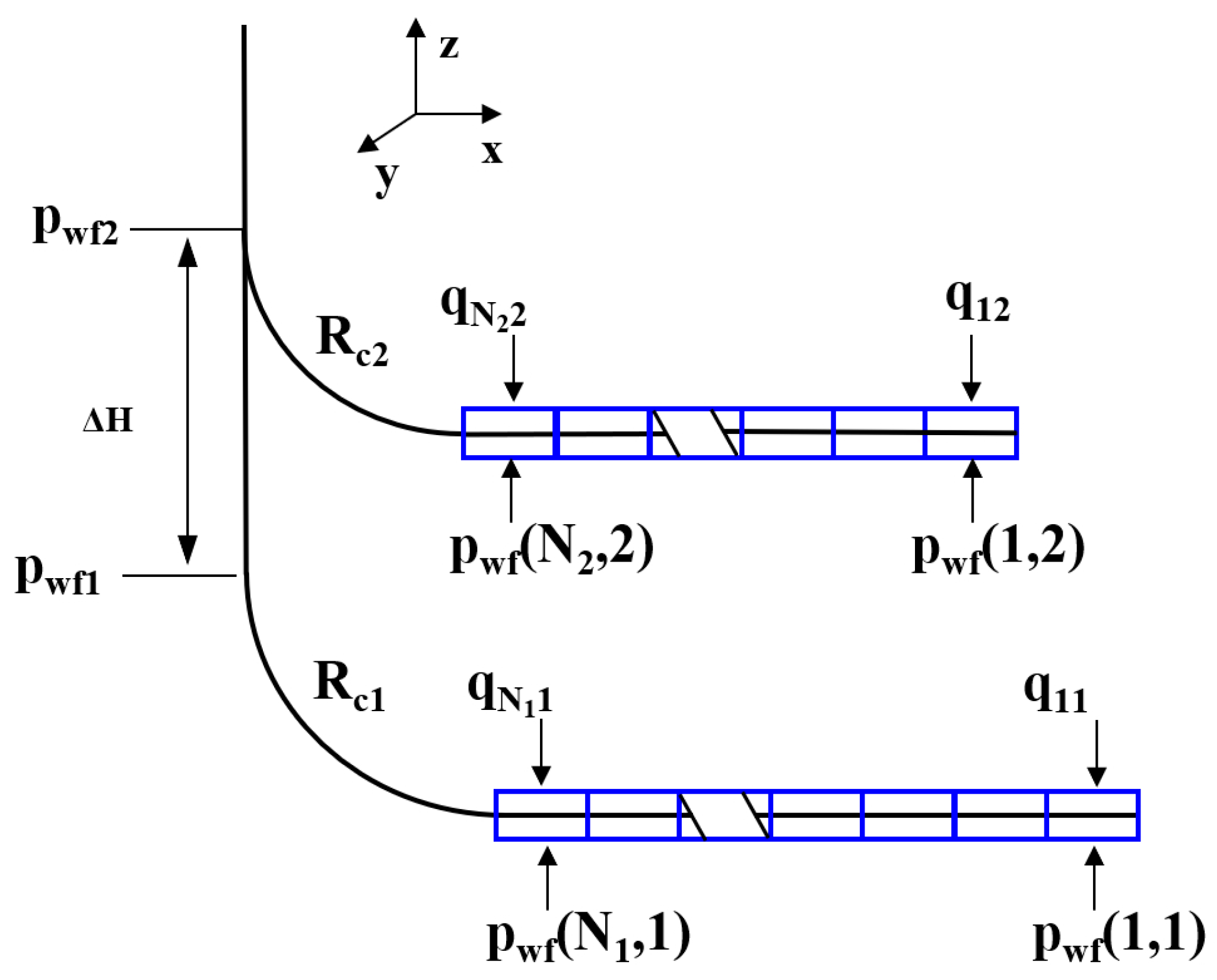
2.2.2. Wellbore Flow Model

The gas flows continuously from the formation into the wellbore, and the mass flow rate within the wellbore increases from the toe end to the heel. The pressure drop in the wellbore includes the wellbore pressure drop, inclined section pressure drop, and vertical wellbore pressure drop.

For a horizontal well with m branches, the laterals are discretized as illustrated in Figure 4. Here, q (i, j) (i = 1, 2, 3…, Nj; j = 1, 2, …, N) is the radial flow rate of the ith microsegment on the branch, p (i, j) is the pressure of the micro-segments, p_wfj is the pressure at the junction of branch j and the vertical wellbore, and R_cj is the radius of the inclined section of the branch j.

(1) Horizontal wellbore pressure drop

Considering the accelerated pressure drop and friction pressure drop, the equation of the pressure drop of the gas flow in the wellbore is [43]

$$\Delta p_{ij}=1.0858\times {10}^{-16}\times \left[{\displaystyle \frac{f\rho {\left(Q_{ij}+q_{ij}/2\right)}^2{L}_{ij}}{D^5}}+{\displaystyle \frac{4\rho q_{ij}\left(Q_{ij}+q_{ij}/2\right)}{D^4}}\right]$$

(16)

$$Q_{gij}={\displaystyle \sum _{i=1}^i{q}_{ij}}$$

(17)

where f is the coefficient of friction; Q_ij is the flow rate of the inflow end of microsegment i; q_ij is the radial flow rate at the inflow end of microsegment i; D is the horizontal well diameter; and L_ij is the length of the microsegment i on branch j.

The coefficient of friction is dependent on the flow regime within the wellbore. The friction coefficient for the laminar flow is [44]

$$f={\displaystyle \frac{16}{N_{\mathrm{Re}}}}(1+0.04304{N_{\mathrm{Re},w}}^{0.6142})$$

(18)

The friction coefficient for the turbulent flow is [44]

$$f=f_o\left(1-0.0153{N_{\mathrm{Re},w}}^{0.3978}\right)$$

(19)

where

$$f_0^{-0.5}=-2\log \left(0.2698{\displaystyle \frac{\epsilon }{D}}-5.0452{\displaystyle \frac{A}{R_e}}\right)$$

(20)

$$N_{\mathrm{Re}}={\displaystyle \frac{2\rho q}{\pi r_w\mu }}$$

(21)

$$N_{\mathrm{Re},w}={\displaystyle \frac{\rho q_s}{\pi \mu }}$$

(22)

where f is the tube flow friction coefficient without the radial inflow; ε is the relative roughness of the pipe’s inside surface; r_w is the radius of the horizontal wellbore; q is the flow rate in the wellbore; q_s is the radial inflow of the wellbore per unit length; ρ is the density of the fluid; and μ is the viscosity of the fluid.

(2) Inclined wellbore pressure drop

Assuming that the flow pressure in the nth micro-segment is P_wf (N_j, j), the inclined wellbore is treated as one fourth of a circle with a radius R_c. During the flow, we consider the gravity pressure drop and friction pressure drop.

The inclined wellbore pressure drop is [45]

$$\begin{array}{c}\Delta p_s={\displaystyle \frac{4\rho f_c{R}_c{q}_m^2}{\pi D^5}}+\rho g{R}_c\end{array}$$

(23)

(3) Vertical wellbore pressure drop

The pressure drop when there is gas–water two-phase productivity in the vertical wellbore is expressed as follows [45]:

$${\displaystyle \frac{\mathrm{d}p}{\mathrm{d}z}}={\rho }_{\mathrm{m}}g+f{\displaystyle \frac{Q_m^2}{2D{A}^2{\rho }_{\mathrm{m}}}}$$

(24)

After integration, the vertical pressure drop can be obtained as shown in Equation (25):

$$\Delta P_v={\rho }_{\mathrm{m}}g\Delta H+f{\displaystyle \frac{q_m^2}{2D{A}^2{\rho }_{\mathrm{m}}}}\Delta H$$

(25)

where ΔH is the height difference between p_wf1 and p_wf2.

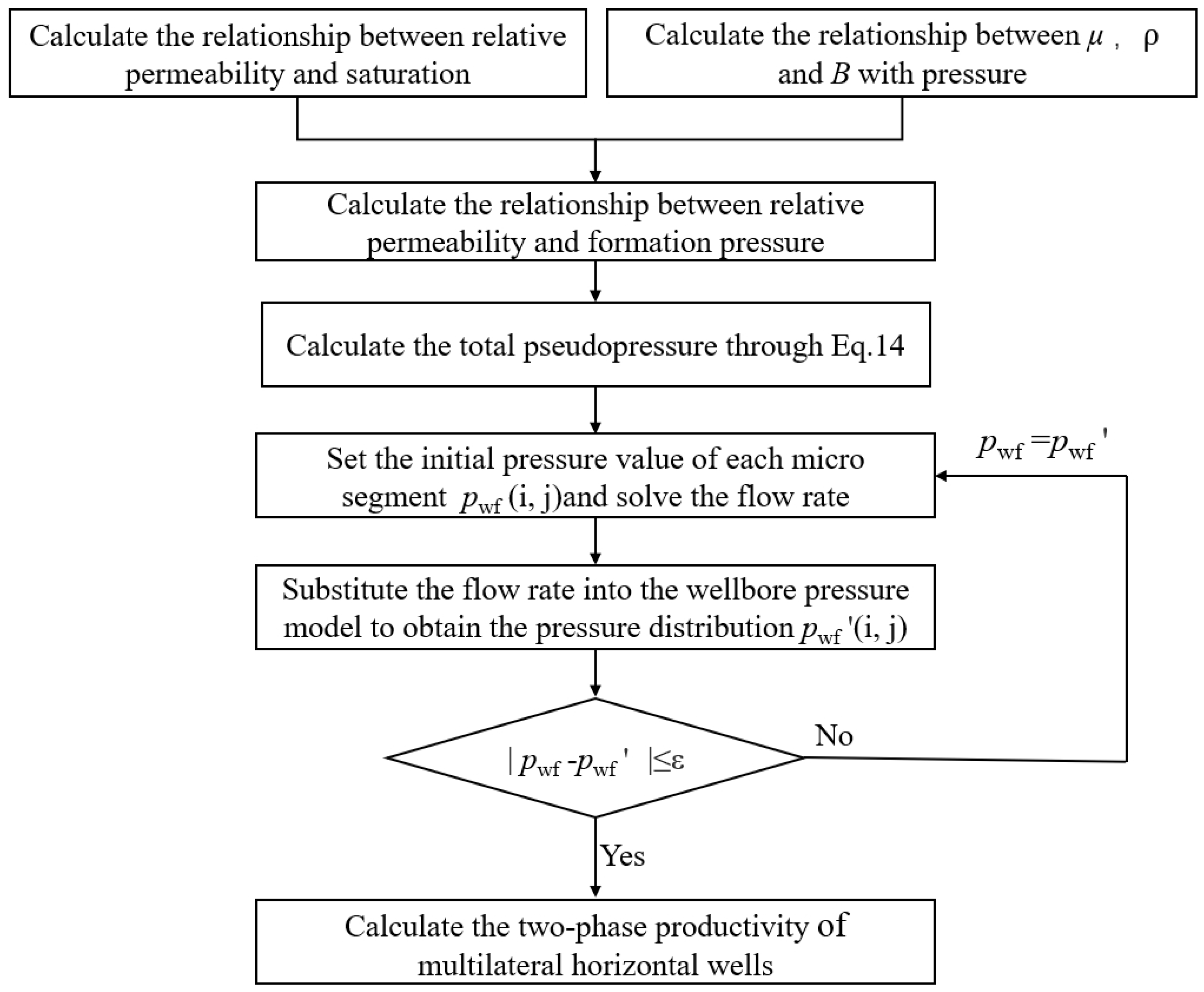
2.3. Coupling Model Solution

The relationship between the relative permeability and pressure is the key to solving the semi-analytical model of multilateral horizontal wells. The relationship between k_rg and k_rw is as follows [42]:

$${\displaystyle \frac{k_{\mathrm{rg}}}{k_{\mathrm{rw}}}}={\displaystyle \frac{B_{\mathrm{g}}{\mu }_{\mathrm{g}}}{B_{\mathrm{w}}{\mu }_{\mathrm{w}}}}·{\displaystyle \frac{1}{R_{\mathrm{wg}}}}$$

(26)

In the case of stable seepage, R_wg remains constant, μ_g and B_g are the functions of pressure, and μ_w and B_w barely change with the pressure. In this paper, they are regarded as constants. The steps to solve the coupling model are outlined in Figure 5, and a pseudo-code flow is added in the Appendix A, which is Figure A1.

3. Results and Discussion

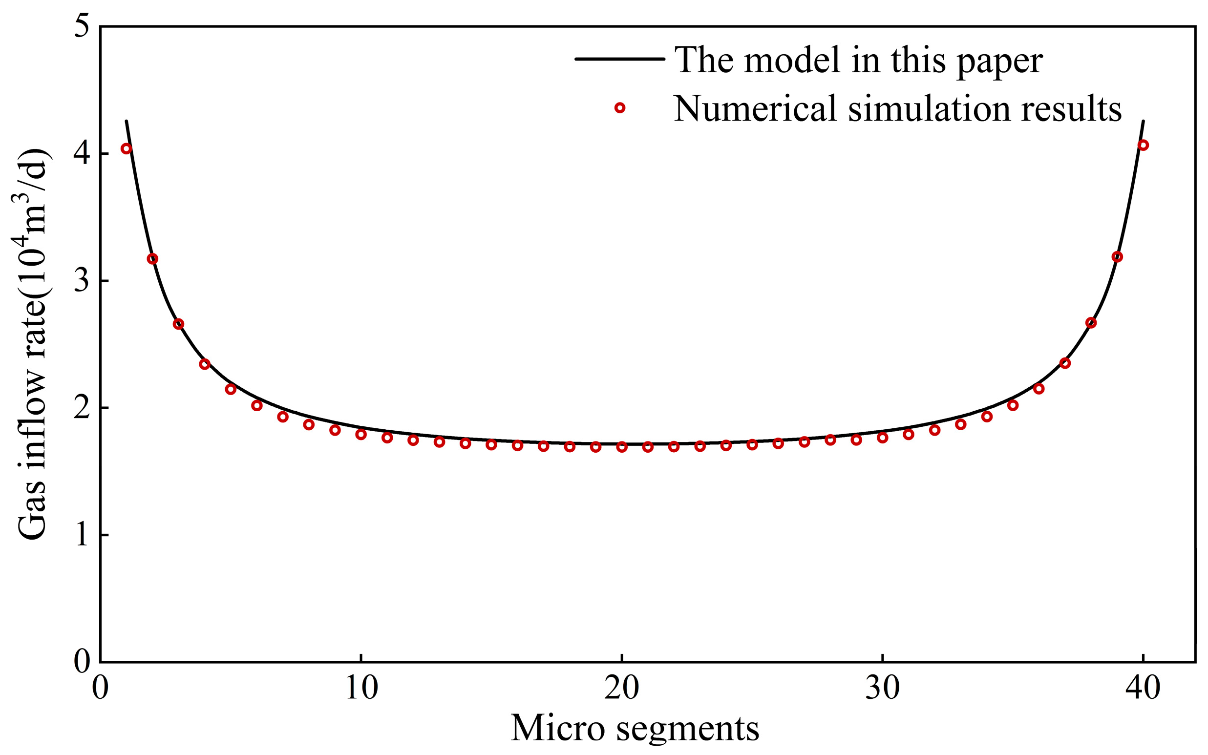
3.1. Coupling Model Solution

To validate the accuracy of the semi-analytical model proposed in this paper, we employed a numerical simulator tNavigator(21.2) to generate a simulation case for horizontal wells. The grid dimension of the numerical simulation was 40 × 40 × 20, and the size of the grid in the x, y, and z directions was 50 m, 50 m, and 0.5 m, respectively. The case adopted the strategy of constant pressure production, and the upper and lower boundaries were closed. The basic parameters of the reservoir and fluids used in the simulation are provided in

Table 1. Basic parameters of reservoir and fluids used in simulation.

Parameters	Value
Initial reservoir pressure (MPa)	16
Initial reservoir temperature (K)	313
Reservoir thickness (m)	10
Reservoir permeability (mD)	50
Initial gas saturation	0.7
Index of gas relative permeability curve	2
Index of water relative permeability curve	3
Water-to-gas volume ratio	0.0001
Initial gas viscosity (mPa·s)	0.02
Initial gas density at standard condition (g/cm3)	0.000732
Initial water density at standard condition (g/cm3)	1
Length of horizontal well (m)	400
Radius of horizontal wellbore (m)	0.108
Curvature radius of horizontal wellbore (m)	15

. The wellbore was divided into 40 micro-segments, and the flow rates at the bottom hole pressure of 14 MPa were calculated. The gas inflow rate distribution of the horizontal well was calculated with the presented coupling model and compared with the results of a numerical simulation, as shown in Figure 6. The gas flow rate distributions along the wellbore obtained by the two methods were consistent, and the gas inflow rate predicted by the proposed model matched the simulation data well, which indicates that the model proposed in this paper has high accuracy in predicting the productivity of horizontal wells in gas reservoirs.

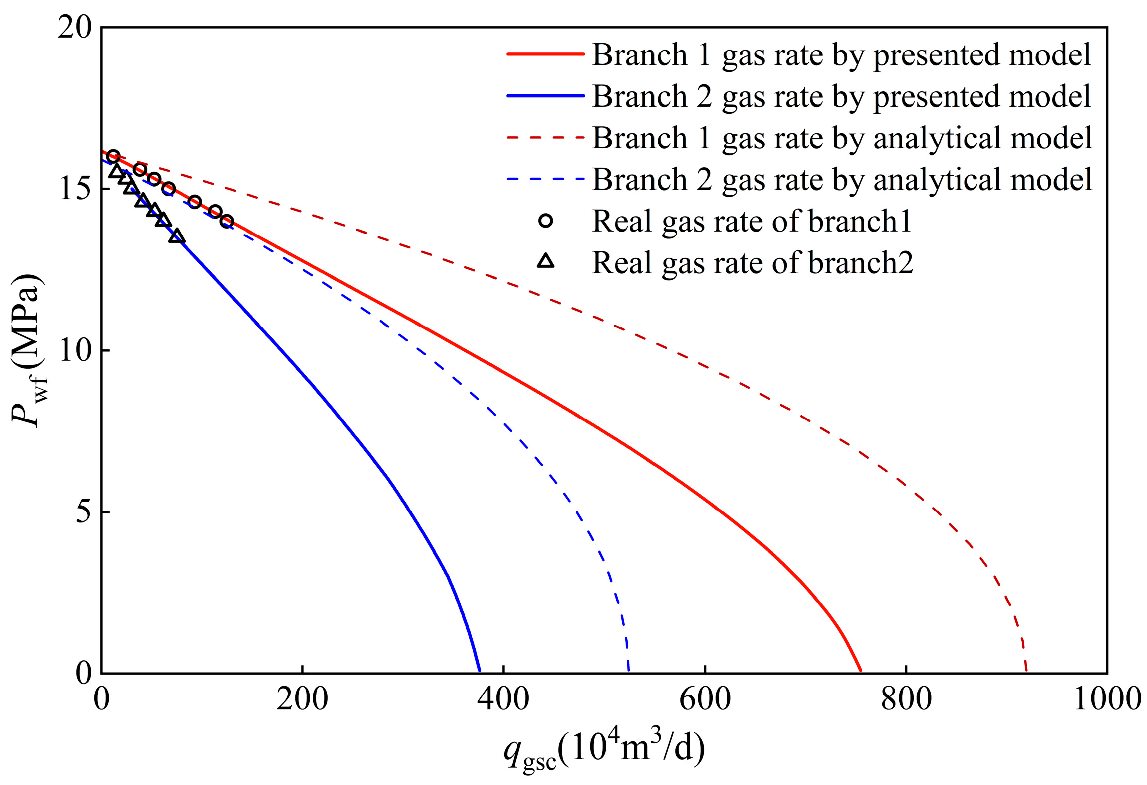
3.2. Field Application

The YM gas field had multiple gas reservoirs in the vertical direction. For the field case, well X31 of the YM gas field was selected. Well X31 was a double-branch horizontal well. Branch 1 was located in the YM2 gas reservoir, and branch 2 was located in the YM1 gas reservoir. The parameters and properties are shown in

Table 2. Basic parameters of reservoir and fluids used in field case.

Parameters	Branch 1	Branch 2
Initial reservoir pressure (MPa)	16.16	15.9
Initial reservoir temperature (K)	313	311
Reservoir thickness (m)	9.72	8.73
Reservoir permeability (mD)	50	43
Initial gas saturation	0.71	0.63
Index of gas relative permeability curve	2	3
Index of water relative permeability curve	3	3
Water-to-gas volume ratio	0.00013	0.00012
Initial gas viscosity (mPa·s)	0.0178	0.0183
Initial gas density at standard condition (g/cm3)	0.000678	0.000679
Initial water density at standard condition (g/cm3)	1	1
Length of horizontal well (m)	606	487
Radius of horizontal wellbore (m)	0.108	0.108
Curvature radius of horizontal wellbore (m)	15	15

. The height difference between the two horizontal branches of well X31 was 50 m.

The current bottomhole pressure of well X31 was 13.5 MPa. When discretizing two horizontal wellbores into 40 micro-segments, the flow distribution of well X31 obtained by the coupling model is shown in Figure 7. It can be observed that the flow rate was higher in the heel and toe regions of the horizontal branch, while it was lower in the middle part of the wellbore. The radial inflow along the production section presented a U-shaped distribution.

Figure 8 shows the pressure difference (ΔP) between the horizontal micro-segments and the wellbore toe as measured by the wellbore flow model. Figure 8 shows that the pressure in the wellbore was not uniform, and the difference increased nonlinearly from the toe to the heel, with a small change in pressure near the toe of the wellbore and a larger change in pressure closer to the heel. This phenomenon occurred because the mass flow rate of the fluid was higher near the wellbore heel, leading to increased friction and acceleration losses in the wellbore, which subsequently resulted in a higher pressure drop.

Additionally, to examine the impact of pressure on the productivity of well X31, the inflow rate of each branch was calculated for various wellbore pressures, and the outcomes are presented in Figure 9. The points in Figure 8 are the real gas data of two branches, which match well with the predicted curve.

Furthermore, in order to investigate the influence of pressure on the productivity of well X31, the inflow velocity of each branch under different wellbore pressures was calculated by using the model proposed in this paper and the analytical model [6] and compared with the actual gas data of the two branches, as shown in Figure 9. Compared with the analytical model of horizontal well productivity, the semi-analytical model proposed in this paper could consider the influence of the wellbore pressure drop, variable flow rate in the wellbore, and water-to-gas ratio on productivity, and it could better match the actual production data, while the results of the analytical model of the horizontal well were larger.

The IPR curves of the two branches of gas well X31 under different water-to-gas ratios, as obtained using the proposed model, are presented in Figure 10 and Figure 11. The productivity of the gas wells was greatly affected by the ratio of water to gas. As the water-to-gas ratio increased, the productivity decreased rapidly. This decrease can be attributed to the increase in water saturation and the subsequent reduction in gas permeability during the two-phase seepage process, ultimately resulting in lower productivity.

4. Conclusions

Based on the existing analytical model, this paper proposed a gas–water two-phase productivity coupling model for multi-branch horizontal wells in multilayer gas reservoirs. Based on the conformal transformation and potential function superposition principle, the model considers the influence of the wellbore pressure drop, variable mass flow rate, and water-to-gas ratio on horizontal well productivity. The following conclusions were obtained:

(1)

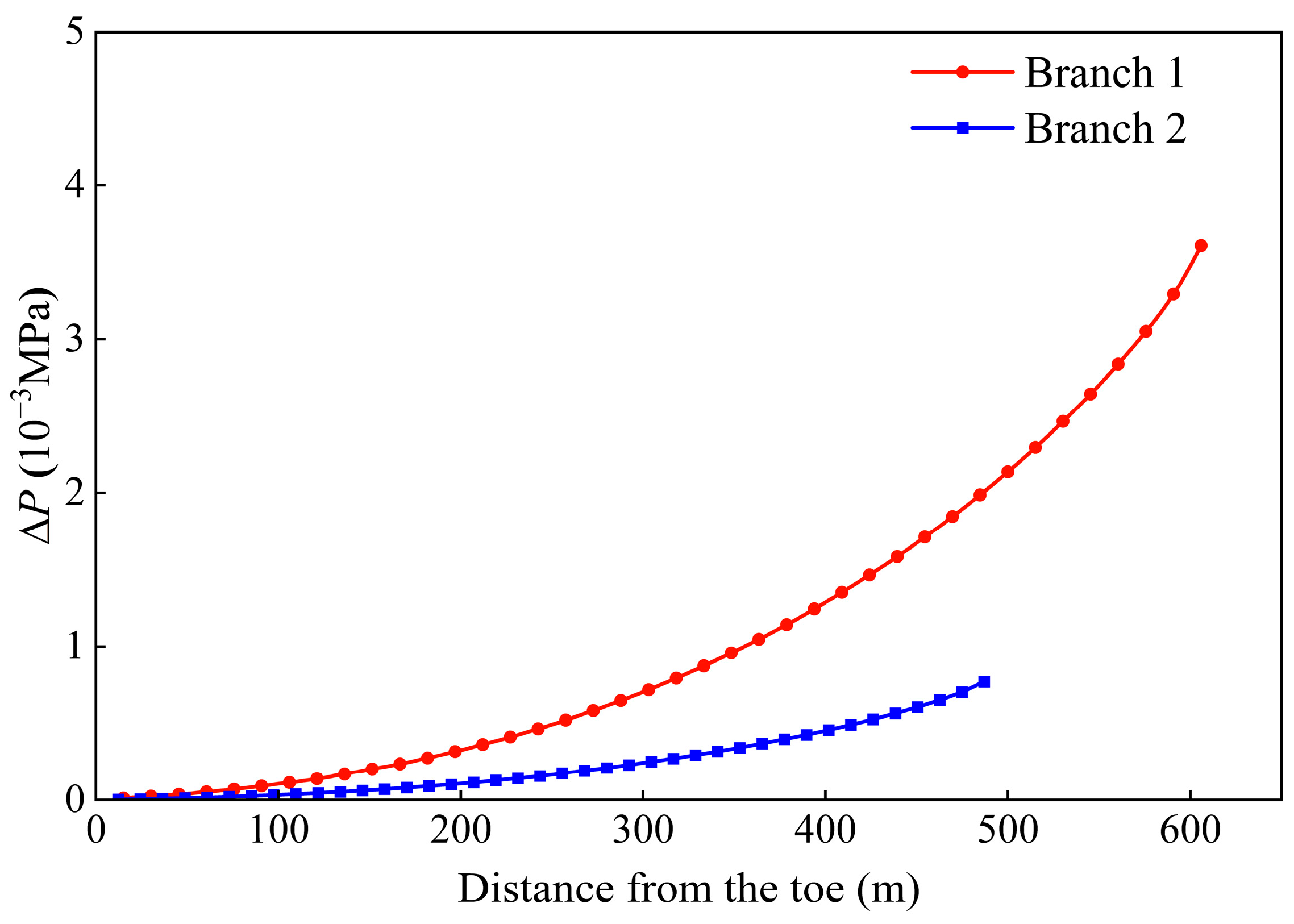
The wellbore flow model utilized in the presented model accounts for both the accelerated pressure drop and friction pressure drop. The results indicate that the pressure in the wellbore was not uniform and increased nonlinearly from the toe to the heel.

(2)

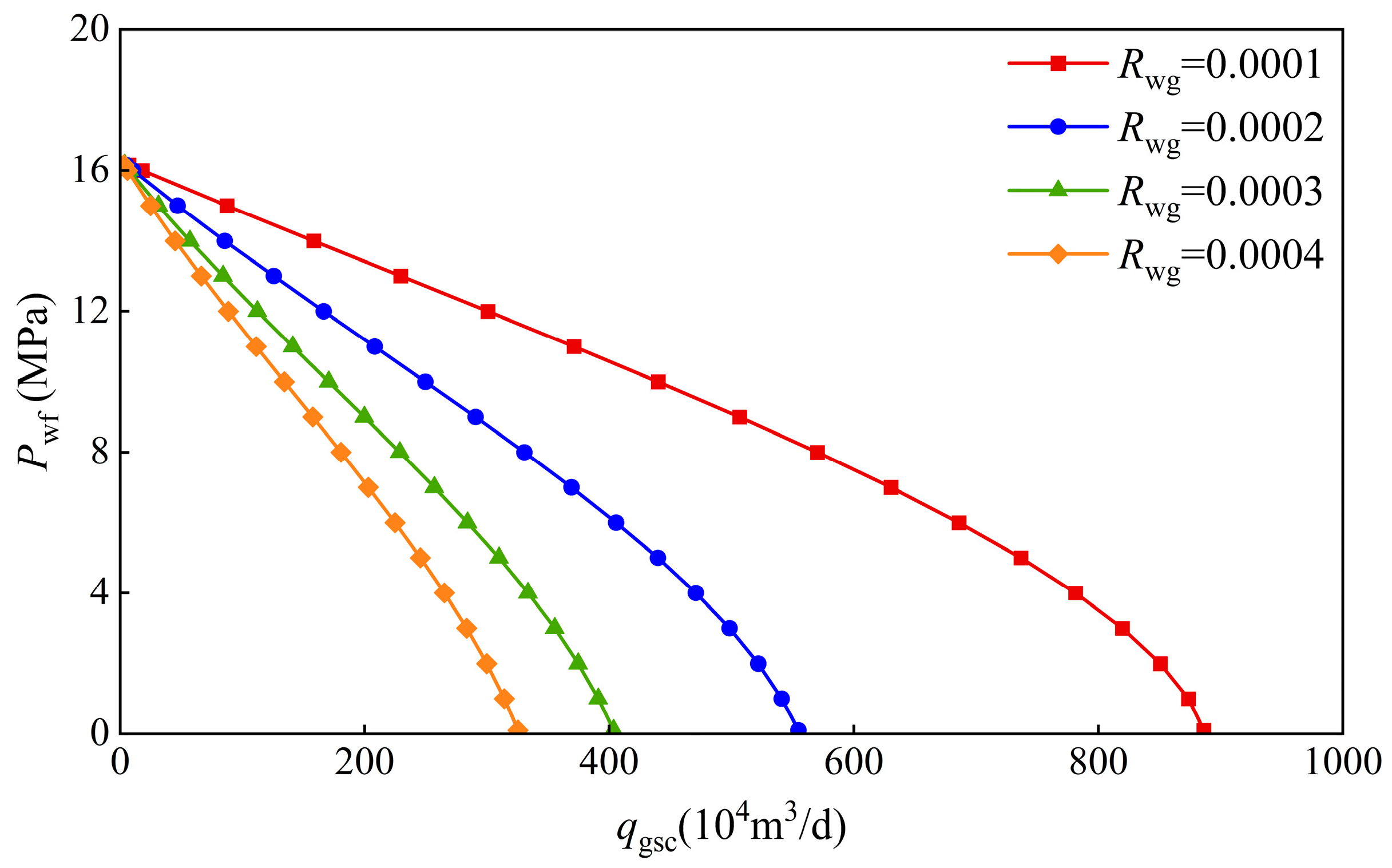
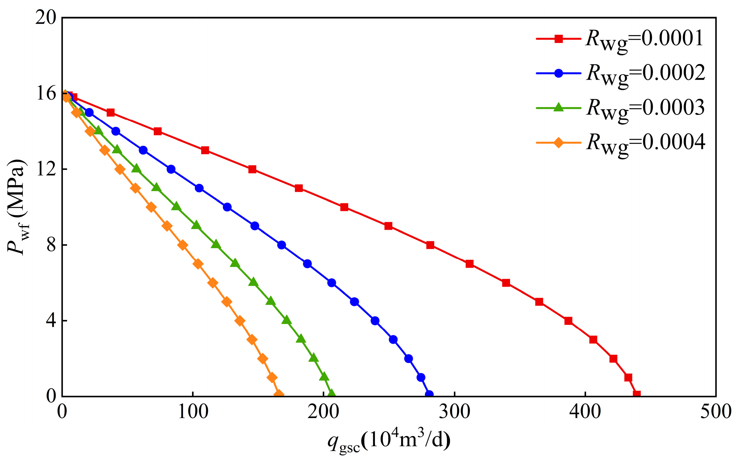
Well X31 in the YM gas field was presented to demonstrate the practical applicability of the proposed approach. The sensitivity analysis shows that the productivity of multilateral wells decreases as the gas-to-water volume ratio increases.

(3)

Compared with the analytical model of horizontal well productivity, the semi-analytical model proposed in this paper can better match the actual production data, while the calculation results of the analytical model of the horizontal well were larger. This is because the model proposed in this paper considers the influence of the wellbore pressure drop, wellbore variable flow, and water-to-gas ratio on productivity.

(4)

In the production process of horizontal wells, reasonable production pressure differences should be controlled to reduce the water production of gas wells and avoid a decline in productivity.

Furthermore, the model proposed in this paper has limitations. Firstly, it does not consider the influence of the fracture network and anisotropy in the formation, which will affect the productivity of horizontal wells. Secondly, this model is suitable for solving the yield of steady state flow without considering a change in the water-to-gas ratio in the production process, which can be further studied.

References

1. Ouyang, L.B.; Aziz, K. A general single-phase wellbore/reservoir coupling model for multilateral wells. SPE Reserv. Eval. Eng. 2001, 4, 327–335. [Google Scholar] [CrossRef]
2. Tabatabaei, M.; Ghalambor, A. A new method to predict performance of horizontal and multilateral wells. SPE Prod. Oper. 2011, 26, 75–87. [Google Scholar] [CrossRef]
3. Hassan, A.; Abdulraheem, A.; Elkatatny, S.; Ahmed, M. New approach to quantify productivity of fishbone multilateral well. In Proceedings of the SPE Annual Technical Conference and Exhibition (D021S012R008), San Antonio, TX, USA, 9–11 October 2017; SPE: Richardson, TX, USA, 2017. [Google Scholar]
4. Wang, Z.; Fu, X.; Guo, P.; Tu, H.; Wang, H.; Zhong, S. Gas-liquid flowing process in a horizontal well with premature liquid loading. J. Nat. Gas Sci. Eng. 2015, 25, 207–214. [Google Scholar] [CrossRef]
5. Zhou, X.; Zeng, F.; Zhang, L. Improving Steam-Assisted Gravity Drainage performance in oil sands with a top water zone using polymer injection and the fishbone well pattern. Fuel 2016, 184, 449–465. [Google Scholar] [CrossRef]
6. Joshi, S.D. Augmentation of well productivity with slant and horizontal wells (includes associated papers 24547 and 25308). J. Pet. Technol. 1988, 40, 729–739. [Google Scholar] [CrossRef]
7. Babu, D.K.; Odeh, A.S. Productivity of a horizontal well. SPE Reserv. Eng. 1989, 4, 417–421. [Google Scholar] [CrossRef]
8. Kong, X.Y.; Xu, X.Z.; Lu, D.T. Pressure transient analysis for horizontal well and multi-branched horizontal wells. In Proceedings of the SPE/CIM International Conference on Horizontal Well Technology, Calgary, AB, Canada, 18–20 November 1996; p. SPE-37069. [Google Scholar]
9. Raghavan, R.; Ambastha, A.K. An assessment of the productivity of multilateral completions. J. Can. Pet. Technol. 1998, 37, 58–67. [Google Scholar] [CrossRef]
10. Wu, J.; Liu, Y.; Yang, H. New Method of Productivity Equation for Multibranch Horizontal Well in Three-Dimensional Anisotropic Oil Reservoirs. J. Energy Resour. Technol. 2012, 134, 032801. [Google Scholar] [CrossRef]
11. Meng, F.; He, D.; Yan, H.; Zhao, H.; Zhang, H.; Li, C. Production performance analysis for slanted well in multilayer commingled carbonate gas reservoir. J. Pet. Sci. Eng. 2021, 204, 108769. [Google Scholar] [CrossRef]
12. Al-Rbeawi, S.; Artun, E. Fishbone type horizontal wellbore completion: A study for pressure behavior, flow regimes, and productivity index. J. Pet. Sci. Eng. 2019, 176, 172–202. [Google Scholar] [CrossRef]
13. Bazitov, M.V.; Golovko, I.S.; Konosov, D.A.; Mingazov, A.N.; Nigmatullin, R.R.; Lokot, A.V.; Malyasov, V.Y. First Fishbone well drilling at Vankorskoe field. In Proceedings of the SPE Russian Petroleum Technology Conference, Moscow, Russia, 26–28 October 2015; p. SPE-176510. [Google Scholar]
14. Cavalcante Filho, J.S.; Xu, Y.; Sepehrnoori, K. Modeling fishbones using the embedded discrete fracture model formulation: Sensitivity analysis and history matching. In Proceedings of the SPE Annual Technical Conference and Exhibition, Houston, TX, USA, 28–30 September 2015; SPE: Richardson, TX, USA, 2015; p. D011S008R006. [Google Scholar]
15. Borisov, J.P. Oil Production Using Horizontal and Multiple Deviation Wells; Nedra: Moscow, Russia, 1964; p. 364. [Google Scholar]
16. Giger, F.M.; Reiss, L.H.; Jourdan, A.P. The reservoir engineering aspects of horizontal drilling. In Proceedings of the SPE Annual Technical Conference and Exhibition, Houston, TX, USA, 16–19 September 1984; OnePetro: Richardson, TX, USA, 1984. [Google Scholar]
17. Dikken, B.J. Pressure drop in horizontal wells and its effect on production performance. J. Pet. Technol. 1990, 42, 1426–1433. [Google Scholar] [CrossRef]
18. Ozkan, E.; Sarica, C.; Haciislamoglu, M.; Raghavan, R. Effect of conductivity on horizontal-well pressure-behavior. SPE Adv. Technol. Ser. 1995, 3, 85–94. [Google Scholar] [CrossRef]
19. Chen, W.; Zhu, D.; Hill, A.D. A comprehensive model of multilateral well deliverability. In Proceedings of the International Oil and Gas Conference and Exhibition in China, Beijing, China, 7–10 November 2000; OnePetro: Richardson, TX, USA, 2000. [Google Scholar]
20. Guo, B.; Zhou, J.; Liu, Y.; Ghalambor, A. A rigorous analytical model for fluid flow in drainholes of finite conductivity applied to horizontal and multilateral wells. In Proceedings of the SPE Oklahoma City Oil and Gas Symposium/Production and Operations Symposium, Oklahoma City, OK, USA, 31 March–3 April 2007; p. SPE-106947. [Google Scholar]
21. Penmatcha, V.R.; Aziz, K. Comprehensive reservoir/wellbore model for horizontal wells. SPE J. 1999, 4, 224–234. [Google Scholar] [CrossRef]
22. Adesina, F.; Paul, A.; Oyinkepreye, O.; Adebowale, O. An improved model for estimating productivity of horizontal drain hole. In Proceedings of the SPE Nigeria Annual International Conference and Exhibition, Lagos, Nigeria, 2–4 August 2016. [Google Scholar]
23. Yan, G.; Li, Z.; Bore, T.; Torres SA, G.; Scheuermann, A.; Li, L. A lattice Boltzmann exploration of two-phase displacement in 2D porous media under various pressure boundary conditions. J. Rock Mech. Geotech. Eng. 2022, 14, 1782–1798. [Google Scholar] [CrossRef]
24. Yan, G.; Bore, T.; Schlaeger, S.; Scheuermann, A.; Li, L. Dynamic effects in soil water retention curves: An experimental exploration by full-scale soil column tests using spatial time-domain reflectometry and tensiometers. Acta Geotech. 2024, 1–27. [Google Scholar] [CrossRef]
25. Yan, G.; Li, Z.; Galindo Torres, S.A.; Scheuermann, A.; Li, L. Transient two-phase flow in porous media: A literature review and engineering application in geotechnics. Geotechnics 2022, 2, 32–90. [Google Scholar] [CrossRef]
26. Vairogs, J.; Hearn, C.L.; Dareing, D.W.; Rhoades, V.W. Effect of rock stress on gas production from low-permeability reservoirs. J. Pet. Technol. 1971, 23, 1161–1167. [Google Scholar] [CrossRef]
27. Jones, F.O.; Owens, W.W. A laboratory study of low-permeability gas sands. J. Pet. Technol. 1980, 32, 1631–1640. [Google Scholar] [CrossRef]
28. Warpinski, N.R. Hydraulic fracturing in tight, fissured media. J. Pet. Technol. 1991, 43, 146–209. [Google Scholar] [CrossRef]
29. Farquhar, R.A.; Smart BG, D.; Todd, A.C.; Tompkins, D.E.; Tweedie, A.J. Stress sensitivity of low-permeability sandstones from the Rotliegendes sandstone. In Proceedings of the SPE Annual Technical Conference and Exhibition, Houston, TX, USA, 3–6 October 1993; p. SPE-26501. [Google Scholar]
30. Texas, A.; Economides, M.J.; Buchsteiner, H.; Warpinski, N.R. Step Pressure Tests for Stress Sensitive Permeability Determination. In Proceedings of the SPE International Conference and Exhibition on Formation Damage Control, Lafayette, Louisiana, 7–10 February 1994. [Google Scholar]
31. Bai, W.; Cheng, S.; Wang, Y.; Cai, D.; Guo, X.; Guo, Q. A transient production prediction method for tight condensate gas wells with multiphase flow. Pet. Explor. Dev. 2024, 51, 172–179. [Google Scholar] [CrossRef]
32. Dou, X.; Liao, X.; Zhao, X.; Wang, H.; Lv, S. Quantification of permeability stress-sensitivity in tight gas reservoir based on straight-line analysis. J. Nat. Gas Sci. Eng. 2015, 22, 598–608. [Google Scholar] [CrossRef]
33. Zhao, K.; Du, P. Performance of horizontal wells in composite tight gas reservoirs considering stress sensitivity. Adv. Geo-Energy Res. 2019, 3, 287–303. [Google Scholar] [CrossRef]
34. Zhao, L.; Jiang, H.; Wang, H.; Yang, H.; Sun, F.; Li, J. Representation of a new physics-based non-Darcy equation for low-velocity flow in tight reservoirs. J. Pet. Sci. Eng. 2020, 184, 106518. [Google Scholar] [CrossRef]
35. Wang, Y.; Wang, J.; Zhao, W.; Ji, P.; Cheng, S.; Yu, H. Explicit Original Gas in Place Determination of Naturally Fractured Reservoirs in Gas Well Rate Decline Analysis. Adv. Geo-Energy Res. 2023, 9, 117–124. [Google Scholar] [CrossRef]
36. Luo, W.; Li, H.T.; Wang, Y.Q.; Wang, J.C. A new semi-analytical model for predicting the performance of horizontal wells completed by inflow control devices in bottom-water reservoirs. J. Nat. Gas Sci. Eng. 2015, 27, 1328–1339. [Google Scholar] [CrossRef]
37. Holmes, J.A.; Barkve, T.; Lund, Ø. Application of a multisegment well model to simulate flow in advanced wells. In Proceedings of the SPE Europec Featured at EAGE Conference and Exhibition, The Hague, The Netherlands, 20–22 October 1998; p. SPE-50646. [Google Scholar]
38. Neylon, K.; Reiso, E.; Holmes, J.A.; Nesse, O.B. Modeling well inflow control with flow in both annulus and tubing. In Proceedings of the SPE Reservoir Simulation Conference, The Woodlands, TX, USA, 2–4 February 2009; p. SPE-118909. [Google Scholar]
39. Wan, J.; Dale, B.A.; Ellison, T.K.; Benish, T.G.; Grubert, M.A. Coupled well and reservoir simulation models to optimize completion design and operations for subsurface control. In Proceedings of the SPE Europec Featured at EAGE Conference and Exhibition, Rome, Italy, 9–12 June 2008; p. SPE-113635. [Google Scholar]
40. Ayesha, A.M.; Hamdy, H. Wellbore segmentation using inflow control devices: Design and optimization process. In Proceedings of the Abu Dhabi International Petroleum Exhibition and Conference, Abu Dhabi, United Arab Emirates, 1–4 November 2010; Society of Petroleum Engineers: Abu Dhabi, United Arab Emirates, 2010. [Google Scholar]
41. Yue, P.; Jia, B.; Sheng, J.; Lei, T.; Tang, C. A coupling model of water breakthrough time for a multilateral horizontal well in a bottom water-drive reservoir. J. Pet. Sci. Eng. 2019, 177, 317–330. [Google Scholar] [CrossRef]
42. Zeng, Y.; Bian, X.Q.; Wang, L.G.; Zhang, L.M. Coupling model of gas-water two-phase productivity calculation for fractured horizontal wells in tight gas reservoirs. Geoenergy Sci. Eng. 2024, 234, 212666. [Google Scholar] [CrossRef]
43. Liu, P.; Wang, Q.; Luo, Y.; He, Z.; Luo, W. Study on a new transient productivity model of horizontal well coupled with seepage and wellbore flow. Processes 2021, 9, 2257. [Google Scholar] [CrossRef]
44. Zeghadnia, L.; Robert, J.L.; Achour, B. Explicit solutions for turbulent flow friction factor: A review, assessment and approaches classification. Ain Shams Eng. J. 2019, 10, 243–252. [Google Scholar] [CrossRef]
45. Yang, J.; Chen, J.; Wang, Q.; Ye, C.; Yu, F. A simple and accurate model to predict pressure drop in vertical gas wells. Energy Sources Part A Recovery Util. Environ. Eff. 2024, 46, 1245–1259. [Google Scholar] [CrossRef]
Figure 1. Two-dimensional seepage zone diagram.
Processes 12 01643 g001
Figure 2. Two-dimensional diagram of horizontal well in y-z section of gas reservoir.
Processes 12 01643 g002
Figure 3. Horizontal well segmentation schematic diagram.
Processes 12 01643 g003
Figure 4. Multilateral horizontal well schematic diagram.
Processes 12 01643 g004
Figure 5. Flowchart of two-phase productivity model of multilateral horizontal wells.
Processes 12 01643 g005
Figure 6. The comparison between the presented model and simulation.
Processes 12 01643 g006
Figure 7. Flow rate distribution in the horizontal wellbore.
Processes 12 01643 g007
Figure 8. Pressure difference distribution in the horizontal wellbore.
Processes 12 01643 g008
Figure 9. Inflow dynamic curve of gas [6].
Processes 12 01643 g009
Figure 10. Branch 1’s inflow dynamic curve of gas.
Processes 12 01643 g010
Figure 11. Branch 2’s inflow dynamic curve of gas.
Processes 12 01643 g011