Solar Water Heating System with Absorption Heat Transformer for Annual Continuous Water Heating

Abstract

We show the performance of solar heating by coupling a Solar Water Heating System (SWHS) with an Absorption Heat Transformer (AHT) for annual continuous water heating. Solar Fraction (SF), Solar Heat Gain (SHG), and Auxiliary Heat (Q_aux) were meticulously assessed for three Mexican cities located in the most characteristic climates (Saltillo, Toluca, and Tapachula). This rigorous assessment process ensures the reliability and accuracy of our findings. The potential reduction in net solar collector area (A_c) and storage tank volume (V_t) can be seen by comparing its annual performance to that of a conventional SWHS. Both configurations were designed to deliver the same hot water amount (0.019 kg/s, 1693.4 L/day, heating from 15.8 to 94.4 °C) and simulated using TRNSYS software version 16.01 concerning combinational systems. The results showed that SWHS-AHT achieved superior performance in solar water heating, achieving a higher SF (up to 99.6%) and SHG (up to 1352 kWh/m²-year) compared to the conventional SWHS. On the other hand, the SWHS-AHT achieved similar performance to a conventional SWHS with up to 60% less A_c. For instance, in Tapachula, a SWHS-AHT with an A_c of 150 m² and a V_t of 18 m³ matched the performance of a SWHS with an A_c of 375 m² and a V_t of 15 m³. Notably, both systems required the same Q_aux. Thus, the Q_aux requirement shows that SWHS-AHT is promising for industrial applications in Mexico, offering improved performance and a reduced footprint.

1. Introduction

Solar energy offers a renewable and sustainable solution, but its intermittent nature and dependence on weather conditions limit its continuous application in industrial processes [1,2]. High upfront costs and lengthy payback periods further complicate its implementation [3]. Despite these challenges, solar energy already contributes to roughly 10% of global primary energy consumption, underscoring its significant potential [4]. Consequently, the development of new technologies to utilize solar energy more efficiently and reliably is crucial [5]. The Absorption Heat Transformer (AHT) emerges as a promising technology to address these challenges, capable of upgrading energy from low-temperature heat sources to higher levels [6,7].

Solar Water Heating Systems (SWHSs) present a highly attractive option for harnessing solar energy, particularly in industrial processes requiring a constant hot water supply [8]. This technology stands out for its wide availability and environmental friendliness [9]. However, SWHSs face significant challenges [10], including intermittency of solar radiation [11], unavoidable thermal losses during storage [12,13], and high initial investment costs [14].

Table 1. Profile of industrial solar water heating systems projects utilizing evacuated tube collectors worldwide.

Project	Location	Year of Operations Start	Installed Net Collector Area, m2	Storage Volume, m3	Installed Thermal Power, kWth	Kind of Fuel Used	Solar Thermal Energy Used for	Temperature Range, °C	Life Time, Year	Solar Fraction, %	Investment Costs, €/m2
Poultry Processing	Simpang Renggam, Malaysia	2017	181.35	8	163.2	−	−	70–75	−	80	498.4
SKZ	Würzburg, Germany	2018	46	6	32.2	−	Hot water bath		−	37	1050.0
Petri	Germany	2018	256	15	179.2	−	−	60	−	34	291.8
Die Badische Staatsbrauerei Rothaus AG	Grafenhausen, Germany	2018	998	50	698.6	Fuel oil	Cleaning bottles and heating water	15–85	−	−	771.5
FIMA Bulking	Klang, Malaysia	2019	481	3	−	Fuel oil	−	−	−	−	427.3
IOI Pan-Century Oleochemicals Sdn Bhd	Jalan Pekeliling, Malaysia	2020	255.75	20	338.25	Natural gas	Pre-heating water to boiler	70–75	−	10	273.7
Clean Energy Heating Project in Shandong Dingtai Animal Husbandry Company	Jinan, China	2020	3825	270	1175	Natural gas	Heating and hot water supply for pig breeding	45–55	25	70	94.1
Rongxing meat and poultry processing	Rongcheng City, China	2021	1018.4	40	712.88	−	Used for hot water requirement of processing workshop	55–60	20	75	173.1
Weishan County Fisheries	Jining city, China	2021	3800	200	2660	−	Used for water heating of nursery pond in fishing ground	25–28	20	60	141.5
Haiyang Zhongtai Garment Factory Project	Jining city, China	2021	5836	360	4085.2	−	Used for rinsing water heating in printing and dyeing rinsing workshop	60–70	−	80	184.3
Dongwang Dairy Farm	Lianyungang City, China	2022	211.5	39	110	−	Producing high-temperature hot water for pasteurization of milk	60–85	15	30	323.8

shows an overview of 11 SWHS projects using evacuated tube collectors, compiled from the Solar Heat for Industrial Processes database [15]. Evacuated tube collectors consistently demonstrate superior Solar Fraction (SF) values compared to other technologies [16], reaching up to 80% [17,18]. SF quantifies the percentage of solar thermal energy utilized relative to the total energy demand [19]. The data reveal a direct correlation between investment costs (€/m²) and the desired temperature range. SWHSs designed to operate within a temperature range of 75–85 °C incur an average cost of 466.8 €/m², while those requiring temperatures below 75 °C have an average cost of 176.9 €/m². Additionally, the analysis highlights the cost implications of achieving high SF values. SWHSs with an SF ranging from 60–80% exhibit an average cost of 218.2 €/m², while systems with an SF between 10–34% have an average cost of 160.5 €/m². In this context, taking advantage of the ability of AHTs to utilize and revalorize solar heat [20] can help a SWHS address these challenges. This approach has the potential to reduce heat losses during storage, minimize the size of collectors and storage tanks, and decrease auxiliary energy consumption. These combined benefits translate to significant cost savings and environmental advantages.

The AHT’s ability to upgrade solar heat has been demonstrated in industrial processes such as seawater desalination [21], steam generation [22], and electricity production [23]. In an experiment of seawater distillation at 94.1 °C, Perez et al. [24] used a SWHS with a Net Collector Area (A_c) of 14 m² of flat plate and a storage tank volume (V_t) of 0.5 m³ to activate an AHT of 1.44 kW. The SWHS supplied hot water at 89.0 °C during a typical day in Cuernavaca, México. The coupling achieved a Coefficient of Performance (COP) of 0.78. In a theoretical seawater desalination process, Salata and Coppi [25] used a variable-area solar pond to activate an AHT. The SWHS provided hot water at 75 °C using an A_c of 4000 m² on a day with Mediterranean climate conditions. The coupling desalinated 1 m³ of water. Gomri [26] used a flat-plate collector system with an A_c of 98.4 m² to activate an AHT in Algeria. The coupling desalinated 0.5 m³ of seawater on a July day, achieving an energy efficiency of 27% and an exergy efficiency of 33%. In a theoretical electricity generation process, Wang et al. [27] proposed a hybrid solar/photovoltaic collector system with an A_c of 160 m² and an AHT activated with waste heat from an internal combustion engine. The coupling achieved the production of steam at 95.0 °C, discontinuously, up to 2687 h per year, with an energy efficiency and exergy efficiency of 56.8% and 33.4%, respectively. In the process of high-temperature steam generation, Wang et al. [28] implemented a flat-plate solar collector system with an A_c of 50 m² to activate a double-absorption AHT. The AHT reached a heating temperature of up to 130 °C in the absorber and a thermal efficiency of 20.3% during a typical day of the year. For their part, Liu et al. [29] coupled a U-type solar collector system with an A_c of 722.6 m² to feed an AHT in Langfang, China. The coupling achieved producing 100 kW of low-temperature steam on a typical summer day. In the process of high-temperature steam generation in Chiang Mai, Thailand, Chaiyat and Kiatsiriroat [30] proposed a solar collector system with an A_c of 70 m² and a V_t of 1.5 m³ coupled to a 10 kW AHT, which in turn works together with a vapor compression heat pump. This thermal system worked 5 h a day during the month of April and reached a COP of 0.71, representing an improvement of 47% over normal solar AHT systems. In general, the results presented indicate that SWHSs coupled with an AHT have the potential to be an energetically viable technology for upgrading solar heat in a variety of industrial processes.

Previous studies have primarily focused on demonstrating the potential of SWHS-AHT to improve system performance through enhanced energy efficiency, exergy efficiency, and/or COP. However, solar heating performance has not been comprehensively assessed. This study addresses this gap by assessing the solar heating performance of a SWHS-AHT for annual continuous water heating. The SF, Solar Heat Gain (SHG), and Auxiliary Heat (Q_aux) are meticulously assessed for three Mexican cities located in the most characteristic climates (Saltillo, Toluca, and Tapachula). Both configurations are designed to deliver the same hot water amount (0.019 kg/s, 1693.4 L/day, heating from 15.8 to 94.4 °C) and simulated using TRNSYS software version 16.01 concerning combinational systems. The potential reduction in A_c and V_t can be seen by comparing its annual performance to that of a conventional SWHS.

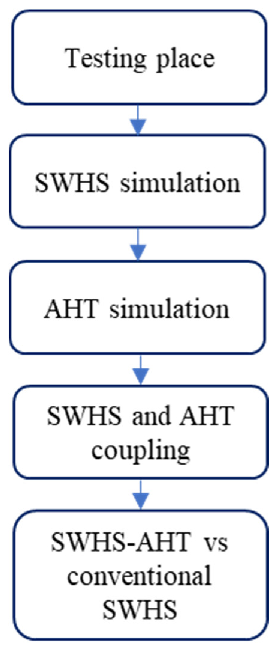
2. Methods and Materials

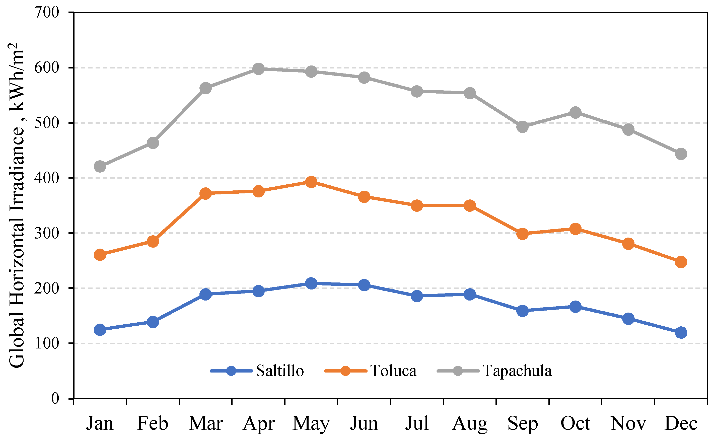
Figure 1 shows the five-step methodology to assess the annual solar heating performance of both SWHS-AHT and conventional SWHSs, considering the specific characteristics and materials of each system. The first step consists of selecting the testing places to ensure geographical and climatic representativeness. Three cities are identified that represent the most characteristic climates of Mexico. Steps two and three involve the simulation of the SWHS and AHT, respectively, considering mass and energy balances. The accuracy of the simulations is then verified by comparing the obtained results with data reported in pertinent literature. In step four, the SWHS and AHT systems are virtually coupled to represent their combined operation. Finally, step five involves a comparative performance analysis of the SWHS-AHT system and a conventional SWHS for annual continuous water heating. This performance assessment incorporates the analysis of SF, SHG, Q_aux, A_c, and V_t.

2.1. Testing Places

Figure 2 shows the three Mexican cities studied (Saltillo, Toluca and Tapachula) with varied climates (semiarid, temperate, and tropical humid) [31] and high Global Horizontal Irradiance (GHI) (1900–2300 kWh/m²-year) [32]. This strategic selection allows for assessing the performance of the system in a diverse spectrum of environmental conditions, ensuring the generalization of the results obtained. The National Meteorological Service (Spanish acronym, SMN) [33] details the climate of each city:

• Saltillo (north): Semiarid, hot summers and cold winters (17 °C annual average). Average annual precipitation: 479.2 mm (summer). Average annual GHI: 2150 kWh/m²-year.
• Toluca (center): Temperate, warm summers and cool winters (12.6 °C annual average). Average annual precipitation: 980 mm (summer). Average annual GHI: 1900 kWh/m²-year.
• Tapachula (southeast): Tropical humid, hot and humid summers, dry and mild winters (27 °C annual average). Average annual precipitation: 2182 mm (summer). Average annual GHI: 2300 kWh/m²-year.

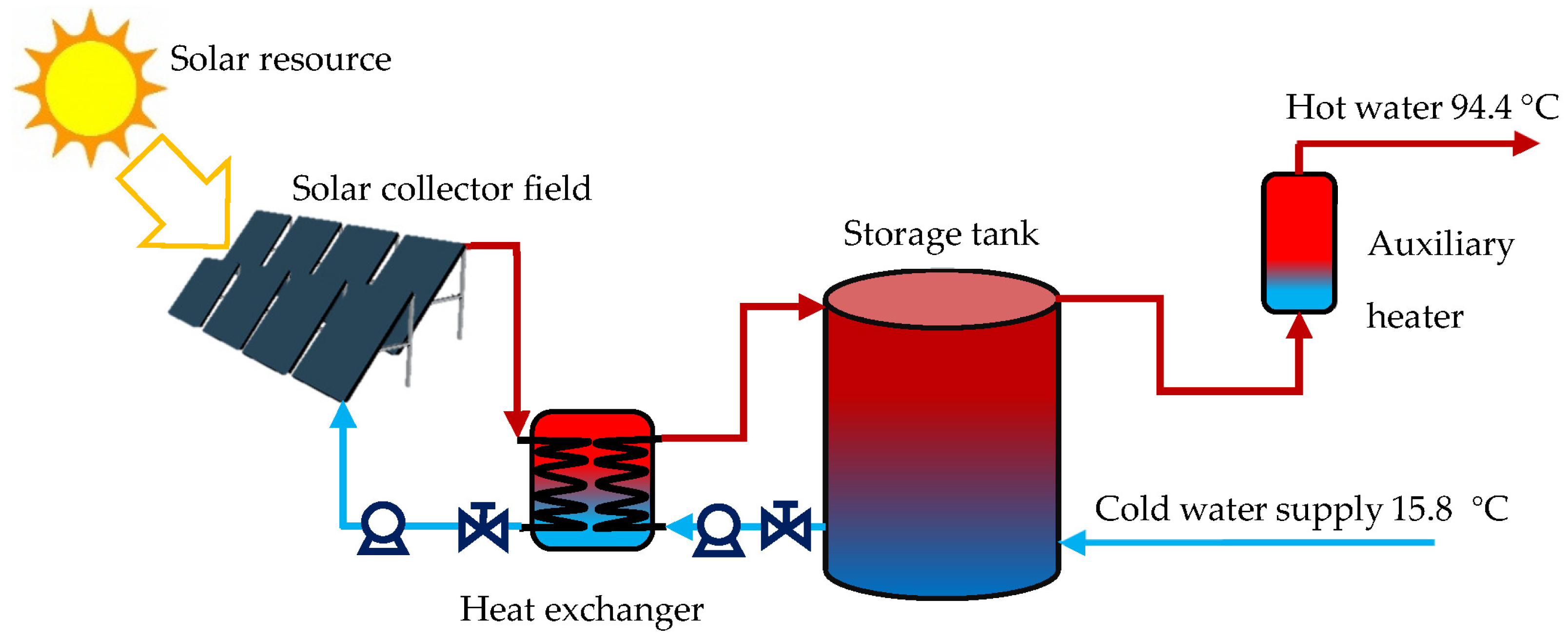
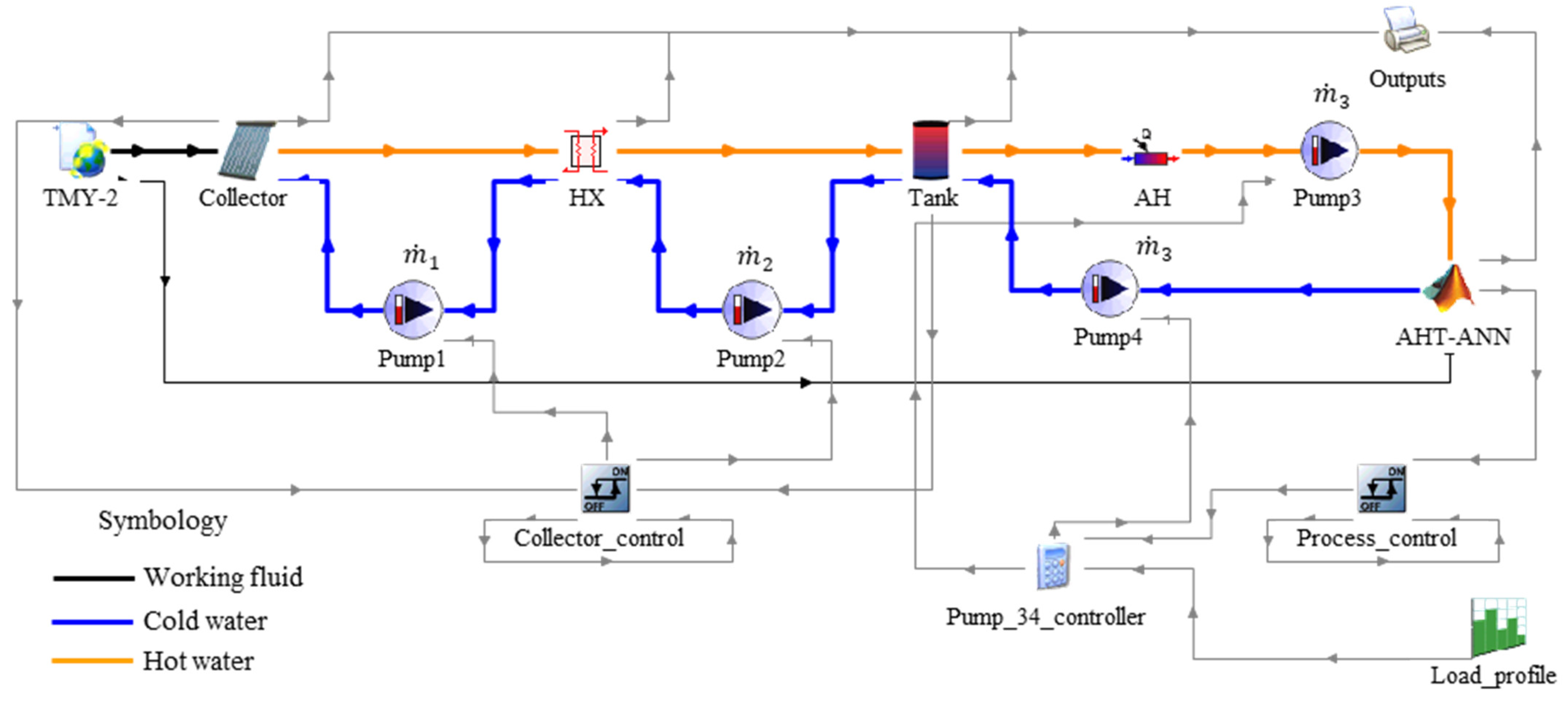
2.2. Solar Water Heating System

2.2.1. Description

Figure 3 shows a schematic representation of the main components of the simulated SWHS for heating water from 15.8 to 94.4 °C continuously throughout the year. The theoretical SWHS corresponds to the configuration proposed by Heß and Oliva [34], validated for a very large company in Würzburg, Germany, working 24 h a day for one year for a high-demand washing or cleaning process. The simulated SWHS consists of a solar collector field, a Heat Exchanger (HE), a vertical stratified hot water storage tank, and an Auxiliary Heater (AH). The solar collector field consists of evacuated tube solar collectors employing a water-ethylene glycol mixture (70% water, 30% ethylene glycol) as the working fluid. The main function of this mixture is to prevent freezing of the heat transfer fluid at low temperatures [35]. The HE utilizes two distinct working fluids: water-ethylene glycol and common water. The storage tank is a vertically stratified cylindrical type with uniform losses, featuring two inputs and two outputs. The AH consists of electrical resistance elements, following Heß and Oliva [34]. These components are modeled in TRNSYS using pre-defined module “Types” with interconnected inputs and outputs aligned with the process flow [36].

Table 2. TRNSYS components for SWHS simulation.

Component	Description	Type	Identifier
Solar resource	Climatological data of a typical year, in TMY-2 format	15-2	TMY-2
Solar collector field	Evacuated tube collector	71	Collector
Heat exchanger	To counterflow	5b	HX
Hydraulic pump	Variable speed pump	110	Pump1, 2, 3 and 4
Storage tank	Stratified, vertical and uniform loss hot water tank	158	Tank
Auxiliary heater	Auxiliary heater with electric resistors	138	AH
Auxiliary element	Calculator tool	−	Pump_34_controller
Load profile	Hot water demand required in the process	14 h	Load_profile
Differential controller, On-Off	On/Off signal	2b	Collector_control
			Process_control
Printer	Represents the output analysis variables in a data sheet	25a	Output
Thermodynamic algorithm	Calls the thermodynamic algorithm implemented in MATLAB	55	AHT-ANN

shows the specific Types employed to simulate each component of the SWHS.

2.2.2. Calculation

The TRNSYS simulation dynamically models the SWHS, accounting for fluctuating weather conditions and their impact on critical parameters like SF and SHG. The SF is determined with Equation (1) and the SHG with Equation (2), following Kalogirou [37].

$$\mathrm{S}\mathrm{F}={\displaystyle \frac{Q_{Solar}}{Q_{Demand}}}\times 100$$

(1)

$$\mathrm{S}\mathrm{H}\mathrm{G}={\displaystyle \frac{Q_{Solar}}{A_c}}$$

(2)

where Q_Solar is the heat obtained by the solar collectors (kWh/year), Q_Demand is the heat demanded by the system (kWh/year) and A_c is the total area of the solar collector field (m²).

The accuracy of the simulated SWHS is assessed by comparing the simulated values of SF and SGH with those reported by Heß and Oliva [34] for Utilization Ratio (UR) from 25 to 75 L/m²-day and Volume Ratio (VR) from 30 to 70 L/m². The coefficient of determination (R²) is used to measure the linear relationship of the data, while a percentage difference analysis determines the magnitude of their differences. The R² is a useful metric for assessing the fit of simulated data. An R² of 0.95 or higher indicates that 95% of the dependent variable is explained by the independent variable [38]. R² is calculated with Equation (3) [39].

$$R^2=1-{\displaystyle \frac{{\sum }_{i=1}^n{(x_i-y_i)}^2}{{\sum }_{i=1}^n{(x_i-\overline{x})}^2}}$$

(3)

where x_i is the target value, $\overline{x}$ it the mean value of x_i, y_i represents the predicted values and n is the data number. UR represents the total amount of fluid passing through each square meter of collector area during a single day (L/m²-day). A high value of UR indicates that the solar collector can satisfy the thermal load, while a low value indicates that the solar collector may not be sufficient. VR, on the other hand, is the ratio of the volume of fluid to be heated to the solar collector area (L/m²). UR and VR depend on the meteorological conditions and are determined by Equations (4) and (5), respectively [40].

$$\mathrm{U}\mathrm{R}={\displaystyle \frac{Demand}{A_c}}$$

(4)

$$\mathrm{V}\mathrm{R}={\displaystyle \frac{V_t}{A_c}}$$

(5)

where Demand is the volume of fluid to be heated daily (L/day), A_c is the total area of solar collectors (m²), and V_t is the volume of the storage tank (L). The mass flow rate ($\dot{m}$) of the pumps is calculated as the product of A_c and UR.

2.3. Absorption Heat Transformer

The AHT simulation considers an Artificial Neural Network (ANN) model to predict temperatures in the main components of an AHT prototype. ANN models have demonstrated significant contributions to improving the COP [41] and efficiency of AHT components [42]. Also, studies have shown that ANN models can achieve high accuracy in temperature prediction for AHT components, with R² values reaching up to 0.996 [43]. R² measures the linear relationship within the data, while a percentage difference analysis determines the magnitude of these differences. As a valuable metric for assessing simulated data fit, an R² of 0.95 or higher indicates that 95% of the dependent variable can be explained by the independent variable [38].

2.3.1. Description

Figure 4 shows the piping and instrumentation diagram of the AHT prototype, depicting the component layout, fluid flow directions, pumps, valves, and sensors. Designed and developed by Varela-Martínez et al. [44], the prototype utilizes an H₂O/LiBr working fluid and is capable of upgrading water temperature from 15.8 to 94.4 °C at a mass flow rate of 0.019 kg/s. The main components of the prototype are a desorber/condenser and an evaporator/absorber, connected by a HE composed of four series-nested helical coils. The system reaches a steady state within a range of 1.2–1.8 h, achieving a COP of 0.18–0.44 and a Gross of Temperature Lift (GTL) of 10.7–24.9 °C. The H₂O/LiBr concentration ranges from 52–56.0%. Heating water reaches 75–81.2 °C while cooling water reaches 15.1–19.8 °C, both maintained at a mass flow rate of 0.1 kg/s. The absorber works at a temperature of 92–108 °C with a mass flow of 0.019 kg/s, and the generator at 71–81.5 °C with a mass flow of 0.015 kg/s. The high-pressure lines work in a steady state at 24.23–41.06 kPa, the low-pressure lines at 5.29–9.07 kPa, and both the cooling and heating water lines run at atmospheric pressure.

The AHT prototype is activated by supplying heat to the medium-temperature weak solution in the desorber (Q_DES) and to the refrigerant in the evaporator (Q_EVA). In the desorber, partial separation of the refrigerant from the working solution occurs when saturation conditions are reached. In the condenser, heat is extracted from the refrigerant externally (Q_CON), causing it to change to a liquid phase and be pumped to the evaporator at an absolute pressure higher than the generator and condenser. The refrigerant is evaporated and fed to the absorber, where it mixes with the concentrated solution from the desorber. In this absorption process, heat is released (Q_ABS) at a higher temperature due to the dilution of the working solution. The heat obtained from the absorption process can be useful for various applications. The diluted solution is fed to the desorber, passing through the economizer to repeat the thermodynamic cycle. The economizer pre-heats the concentrated solution by utilizing the thermal level of the diluted solution, providing the absorber with a higher input temperature, thereby enhancing the exothermic reaction and consequently improving the AHT’s performance.

Table 3. Data set statistical descriptors.

Parameter	Sensor	Description	Mean	SD	Min.	Max.
Temperature, °C	T1	Desorber heating water input temperature	75.8	10.9	23.0	86.8
	T2	Desorber heating water output temperature	71.6	10.4	22.8	81.8
	T3	Condenser cooling water input temperature	20.0	3.1	12.7	29.8
	T4	Condenser cooling water output temperature	22.0	3.7	12.5	32.1
	T5	Evaporator heating water input temperature	76.5	10.7	22.0	95.1
	T6	Evaporator heating water output temperature	72.9	10.1	22.6	94.4
	T7	Absorber useful water input temperature	24.7	7.0	15.7	70.6
	T8	Absorber useful water output temperature	73.9	29.9	16.1	111.4
	T9	Desorber refrigerant output temperature	56.2	11.1	21.8	71.8
	T10	Condenser refrigerant output temperature	31.1	5.5	15.2	47.7
	T11	Evaporator refrigerant input temperature	31.6	5.6	20.3	62.7
	T12	Evaporator refrigerant output temperature	48.0	11.0	21.0	75.0
	T13	Absorber weak solution output temperature	80.5	22.9	15.3	123.0
	T14	Desorber weak solution input temperature	60.7	15.5	18.4	82.0
	T15	Desorber strong solution output temperature	66.3	13.6	23.3	85.6
	T16	Absorber strong solution input temperature	69.8	19.3	22.6	107.0
Pressure, kPa	PLOW	Low-pressure line	3.7	2.6	2.6	12.7
	PHIGH	High-pressure line	20.6	10.1	1.3	43.3
Mass Flow, kg/s	${\dot{m}}_{CON}$	Condenser mass flow rate	4.5 × 10−4	3.14 × 10−4	5.3 × 10−5	2.2 × 10−3
	${\dot{m}}_{DES}$	Desorber mass flow rate	4.2 × 10−2	0.1	1.8 × 10−5	0.93
	${\dot{m}}_{ABS}$	Absorber mass flow rate	2.3 × 10−2	4.5 × 10−2	2.4 × 10−5	0.89
Concentration, %	XSTRONG	Strong solution concentration LiBr/H2O	59.8	4.2	48.8	69.4
	XWEAK	Weak solution concentration LiBr/H2O	57.1	4.9	45.0	67.4

shows a description of the thermal parameters measured during the experimental tests carried out by Martínez-Varela et al. [44]. Measurements were recorded every 10 s using an Agilent data logger and BenchLink Data Logger Pro 3.3 software. Data were collected from 20 experimental tests that reached steady-state conditions within a timeframe of 1.2–1.8 h. The high standard deviation is attributable to data collection beginning during the AHT’s transient start-up phase and continuing until a steady state was achieved. The data set corresponds to 27,426 temperatures at the inputs and outputs of the components, the pressures in the high and low lines, and the mass flow at the input of the condenser. Temperature measurements were obtained using PT-1000 West sensors with an accuracy of ±0.3 °C, while pressure measurements were recorded with Cole-Parmer pressure transducers with an accuracy of ±0.13%. The condenser mass flow rate was measured by a McMillan digital flowmeter with an accuracy of ±1%. Mass flow rates at the desorber and absorber outputs were recorded only when the AHT reached a steady state. Similarly, concentrations were measured manually using an Atago brand mass refractometer, with an accuracy of ±0.1%. Finally, the mass flow rates of heating water, cooling water, and useful heat water were measured with Blancett turbine flowmeters, all having an accuracy of ±0.1%.

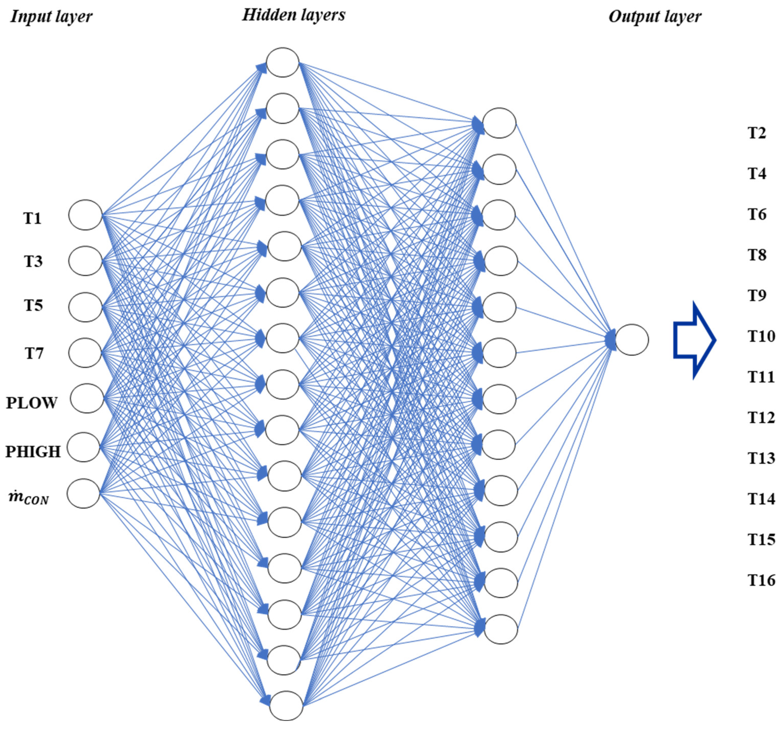
2.3.2. Calculation by ANN

This study develops an ANN-based model for the AHT, referred to as AHT-ANN. Table 3 shows a statistical description of the predicted and predictor employed in the AHT-ANN. The predicted variables comprise the output temperatures of the cooling and heating water, along with the input and output temperatures of the refrigerant and working solution in each main component of the AHT (T2, T4, T6, T8, T9, T10, T11, T12, T13, T14, T15, T16). The predictor variables encompass the pressures within the main components, condenser mass flow rate, and the input temperatures of the heating and cooling water (T1, T3, T5, T7, PLOW, PHIGH, $\dot{m}$_CON). The predicted temperatures from the model were subsequently used in conjunction with a proposed thermodynamic algorithm to calculate the heat fluxes and COP.

The AHT-ANN development follows the methodology proposed by López-Pérez et al. [39] and is implemented using MATLAB software (R2016a) [45]. This methodology covers architecture selection, training method, hyperparameter tuning, and optimization. The AHT-ANN architecture is a multilayer perceptron with an input layer, one or more hidden layers, and an output layer. The number of hidden layers is determined through the optimization process. The input layer comprises seven neurons corresponding to the number of predictor variables. Initially, the hidden layer consists of two neurons, with the potential to increase during optimization. The output layer has 12 neurons, aligning with the number of predicted variables. Both the input and output layers utilize the Purely Linear (PURELIN) transfer function. Initially, the hidden layer employs the Logarithm of the Sigmoid (LOGSIG) as its activation function. However, the optimization process also evaluates the Tangent Sigmoid (TANSIG) function for the hidden layer.

The AHT-ANN model applies a supervised learning approach with feedback training. The Backpropagation algorithm facilitates weight adjustments between neurons during the training process. For weight optimization, the Levenberg–Marquardt algorithm is utilized. The training process consists of 1000 times-epochs, aiming for a minimum error goal of 0.0. Hyperparameter tuning involves optimization of the learning rate, momentum, and k-value for k-fold cross-validation. During initial model training and subsequent performance evaluation, a parametric variation is applied to the learning rate and momentum, ranging from 0.1 to 1.0. This initial model incorporates the previously established set of 7 predictors and 12 predicted variables. Selection of the final learning rate and momentum values prioritizes the model achieving the highest R² and the lowest Mean Absolute Error (MAE). Equation (6) calculates the MAE [39].

$$\mathrm{M}\mathrm{A}\mathrm{E}={\displaystyle \frac{1}{n}}{\sum }_{i=1}^n\left|y_i-x_i\right|$$

(6)

where x_i is the target value, $\overline{x}$ is the mean value of x_i, y_i is the predicted values, and n is the total number of data points.

The k-fold cross-validation method is employed within the machine learning framework to establish optimal data divisions for training and validating the ANN model. This approach promotes generalizability and minimizes overfitting risks. The selection of the optimal k-value focuses on the development and evaluation of the initial model’s fit. The data set is divided iteratively from 2 to 20 folds (k-value). The chosen k-value corresponds to the iteration that achieves the best fit, as measured by the R² and MAE.

The optimization process of the AHT-ANN model focuses on achieving superior precision and stability in predicting target variables while avoiding underfitting and overfitting. This iterative process involves training the initially proposed model with pre-defined parameters, followed by variations in the number of neurons and transfer functions within the hidden layer. Each iteration undergoes performance evaluation using R² and MAE metrics. The optimization process terminates when a configuration achieves the highest R² and the lowest MAE, signifying successful optimization.

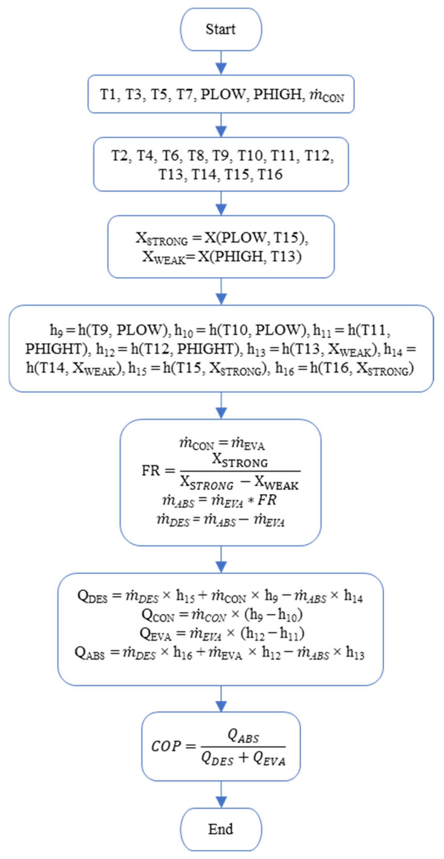
2.3.3. Thermodynamic Algorithm

Figure 5 shows the flow diagram of the thermodynamic algorithm implemented in MATLAB to calculate the heat fluxes and the COP of the AHT-ANN model, following Delgado-Gonzaga et al. [46]. The algorithm considers the mass, material and energy balances through Equations (7), (8), and (9), respectively [47]. In all simulations, T1 is assumed to be equal to T5, while T3, T7, PLOW, PHIGH and $\dot{m}$_CON take the average values provided in Table 2.

$${\sum }_{in}\dot{m}-{\sum }_{out}\dot{m}=0$$

(7)

$${\sum }_{in}\dot{m}X-{\sum }_{out}\dot{m}X=0$$

(8)

$${\sum }_{in}\dot{m}h-{\sum }_{out}\dot{m}h+\dot{Q}+\dot{W}=0$$

(9)

2.4. SWHS and AHT Coupling

Figure 6 shows the TRNSYS platform developed to simulate the performance of both the SWHS and the SWHS-AHT systems. The SWHS process is initiated by the TMY-2 weather data file, which supplies the collector with solar radiation and environmental data for a typical year. The collector heats the working fluid and delivers it to the Heat Exchanger (HX) at a mass flow rate $\dot{m_1}$. Within the HX, the hot working fluid transfers heat to the cold water stored in the tank. Pump1 then circulates the cooled working fluid back to the collector, completing the primary loop. Hot water is stored in the tank, while Pump2 draws cold water from the tank and delivers it to the HX at a mass flow rate $\dot{m_2}$, completing the secondary loop. Pump3 extracts hot water from the tank at a mass flow rate, $\dot{m_3}$, and feeds it to the AHT-ANN model. The AH serves as a supplementary heat source, providing Q_aux when solar energy is insufficient to meet the desired water temperature. Finally, Pump4 returns the cooled working fluid from the AHT-ANN process back to the tank, completing the tertiary loop.

The AHT-ANN model replicates the processes of a conventional AHT. The output component stores relevant parameters in a data file for further performance evaluation. The Collector_control component ensures Pump1 and Pump2 only operate when the working fluid entering the tank is hotter than the stored working fluid. Process_control and Pum_34_controller manage Pump3 and Pump4 operation based on system demand (Load_profile) and a maximum temperature threshold of 95 °C, as outlined by Varela-Martínez et al. [44]. Type55 serves as a link to the external AHT simulator (details provided in Table 3).

Table 4. Parameters and thermal characteristics of simulated components.

Component	Parameter	Value
TMY-2	Environmental conditions for a typical year	TMY-2 format
Collector	Type	Evacuated tubes
	Net collector area	Variable
	Fluid heat carrier (70% water, 30% ethylene glycol)	Density, 1035 kg/m3
		Specific heat, 3.72 kJ/kg K
	Efficiency parameters	First-term solar collector thermal efficiency equation (dimensionless), 0.811
		Second-term solar collector thermal efficiency equation, 2.71 W/m2 K
		Third-term solar collector thermal efficiency equation, 0.01 W/m2 K
	Azimuthal angle, °	In front of the Equator
	Tilt angle	18 °
HX	Flow direction	Counterflow
	Fluid heat carrier (70% water, 30% ethylene glycol), cold side	Density, 1035 kg/m3
		Specific heat, 3.72 kJ/kg K
	Fluid heat carrier (water), hot side	Density, 1000 kg/m3
		Specific heat, 4.19 kJ/kg K
	Heat transfer coefficient	24 kW/K
Pump1	Working fluid	70% water, 30% ethylene glycol
	Capacity	6000 kg/h
	Rated power	6 kW
	Use efficiency	0.6
	Engine efficiency	0.9
Pump1, 2, 3 and 4	Working fluid	Water
	Capacity	6000 kg/h
	Rated power	5 kW
	Use efficiency	0.6
	Engine efficiency	0.9
Tank	Type	Vertically stratified thermostatic storage tank
	Volume	Variable
	Working fluid, water	Density, 1000 kg/m3
		Specific heat, 4.19 kJ/kg K
	Heat transfer coefficient,	0.83 kJ/h m2 K
	Stratification sections	5
AH	Working fluid, water	Density, 1000 kg/m3
		Specific heat, 4.19 kJ/kg K
	Efficiency	0.8

summarizes the main parameters and thermal characteristics of the simulated system components.

2.5. Comparative Parameters

Table 5. SWHS-AHT and SWHS comparative.

System	Storage Tank Requirements				Useful Water Production
	Demand, L/day	${\dot{\mathit{m}}}_3$, kg/s	Tint, °C	Tout, °C	Demand, L/day	${\dot{\mathit{m}}}_{\mathit{u}\mathit{s}\mathit{e}}$, kg/s	Tint, °C	Tout, °C
SWHS-AHT	17,280	0.2	15.8	81.2	1693.4	0.019	15.8	94.4
SWHS [44]	1693.4	0.019	15.8	94.4

shows the thermal operating parameters of the SWHS-AHT system compared to a conventional SWHS for annual continuous water heating. These parameters correspond to the optimum performance values recorded by the AHT prototype developed by Varela-Martínez et al. [44]. Both systems operate continuously, heating water from 15.8 to 94.4 °C with a constant mass flow rate, $\dot{m}$_USE, of 0.019 kg/s throughout the year throughout the year to deliver 1693.4 L/day for an industrial process. The AHT prototype requires 17,280 L/day of hot water at 81.2 °C with a mass flow rate, ${\dot{m}}_3$, of 0.2 kg/s (desorber and evaporator). This configuration achieves a temperature difference (ΔT) of 13.2 °C and a COP of 0.44. The SWHS-AHT and the conventional SWHS utilize a Q_aux to meet energy demands during periods without solar radiation. The simulated environmental conditions are derived from the Meteonorm database (version 7.1) and correspond to a typical year [48]. The performance of both systems is evaluated based on SF, SHG, Q_aux, A_c, and V_t. Additionally, values for ${\dot{m}}_1$ and ${\dot{m}}_2$ are proposed. The simulated environmental conditions come from the Meteonorm database version 7.1 and correspond to a typical year.

The A_c and V_t for both the SWHS-AHT and the conventional SWHS are determined based on the thermal parameters specified for producing the required useful water. This process involves iteratively establishing values for UR and VR [34]. The performance of the proposed dimensions for each UR and VR value is assessed based on the SF and SHG. The objective is to identify combinations that maximize both parameters.

3. Results and Discussion

This chapter shows the results of the assessment of solar heating performance by coupling an SWHS and an AHT for annual continuous water heating. The evaluation focuses on three Mexican cities representing the most characteristic climates and analyzes key parameters: SF, SHG, and Q_aux. The performance of the simulation platforms developed for SWHS and AHT has been assessed. By comparing the annual performance metrics (SF, SHG, and Q_aux) of the SWHS-AHT system with the conventional SWHS, the potential reduction achievable in A_c and V_t was explored. Given the novelty of this approach for continuous industrial hot water heating, individual comparisons were made between systems based on the above criteria.

3.1. SWHS Simulation Platform

Figure 7 compares the performance of the simulated SWHS with the theoretical SWHS in terms of SF and SHG, with a UR of 25 to 75 L/m²-day and a VR of 30 to 70 L/m². In SF, an R² of 0.99 was reached for all the UR and VR intervals, with maximum differences of less than 5.0%. Regarding SHG, R² was from 0.98 to 0.99 for all UR and VR intervals, with a maximum difference of 28.1 kWh/m²-year. The results show that the simulation platform is a reliable tool for predicting SWHS performance under different climatic conditions. Furthermore, it can be used to evaluate SWHS performance in different cities and regions of the world, as well as to optimize system design.

3.2. Absorption Heat Transformer Simulation

Table 6. Initial AHT model performance during parameter selection and optimization.

Hyperparameter Selection
	Coefficient	0.1	0.2	0.3	0.4	0.5	0.6	0.7	0.8	0.9	1
Learning rate	R2, −	0.900	0.912	0.912	0.935	0.926	0.925	0.927	0.923	0.922	0.921
	MAE, °C	4	3.8	3.9	3.6	3.8	3.8	3.8	4	3.9	4
Momentum	R2, −	0.91	0.927	0.923	0.922	0.9208	0.940	0.924	0.925	0.925	0.925
	MAE, °C	3.8	3.8	4	3.9	4	3.6	3.8	3.8	3.8	3.7
k-Value Selection
	k	2	4	6	8	10	12	14	16	18	20
	R2, −	0.905	0.923	0.920	0.930	0.928	0.928	0.915	0.924	0.921	0.922
	MAE, °C	4	3.8	3.5	3.2	3.4	3.6	3.6	3.8	3.8	3.9
AHT-ANN Optimization
	Neuron	2	4	6	8	10	12	15	16	18	20
LOGSIG	R2, −	0.866	0.886	0.901	0.914	0.926	0.918	0.951	0.951	0.950	0.950
	MAE, °C	7.2	5.6	4.9	4.3	4	3.6	2.8	2.8	2.8	2.9
TANSIG	R2, −	0.866	0.885	0.904	0.916	0.93	0.933	0.964	0.964	0.954	0.952
	MAE, °C	7.2	5.6	4.8	4.2	3.6	3.4	2.7	2.7	2.8	2.8

shows a comparison of the performance of the initial AHT-ANN model during hyperparameter selection and optimization. The evaluation was based on the R² and MAE metrics. The learning rate and momentum that achieved the highest R² and the lowest MAE were 0.4 and 0.6, respectively. The selected k-value was 8, resulting in an R² of 0.930 and an MAE of 3.2 °C. The optimized AHT-ANN model employs 15 neurons in the hidden layer with TANSIG transfer functions. This configuration achieved a superior R² of 0.964 and a lower MAE of 2.7 °C.

Figure 8 shows a schematic representation of the optimized AHT-ANN model. The optimized AHT-ANN has 15 neurons in the hidden layer with TANSIG transfer functions. The input layer has seven neurons, and the output layer has 12 neurons, both with PURELIN transfer functions.

Equation (10) shows the proposed model in matrix form, illustrating the PURELIN–TANSIG–PURELIN configuration [49].

$$Y=W_2\left[{\displaystyle \frac{2}{1+e^{-2(W_{1}X+b_1)}}}-1\right]+b_2$$

(10)

where Y is a 12 × 1 output vector, X is a 7 × 1 input vector, W₁ is a 15 × 12 weight matrix in the hidden layer, b₁ is a 15 × 1 bias vector in the hidden layer, W₂ is a 12 × 15 weight matrix in the output layer, and b₂ is a 12 × 1 bias vector in the output layer.

Figure 9 shows the fit of the temperatures predicted by the optimized AHT-ANN model and the target variables with the whole data set. The results demonstrate that the utilized set of predictor variables can adequately predict the target temperatures in the main components. This is evidenced by an average R² of 0.964 and an average MAE of 2.7 °C. Furthermore, the individual follow-up analyses for each predicted variable reveal a good fit. The R² and MAE values for each temperature are as follows: T2 (0.980, 1.5 °C), T4 (0.956, 0.9 °C), T6 (0.980, 1.5 °C), T8 (0.973, 4.5 °C), T9 (0.960, 3.2 °C), T10 (0.963, 2.6 °C), T11 (0.940, 2.8 °C), T12 (0.960, 4.2 °C), T13 (0.977, 3.5 °C), T14 (0.947, 3.9 °C), T15 (0.966, 2.9 °C), and T16 (0.970, 3.2 °C).

3.3. Performance Comparison of SWHS-AHT and Conventional SWHS

3.3.1. Optimal Configurations

The best-performing SWHS-AHT configurations utilized specific operating parameters. These optimal configurations involved UR ranging from 49.4 to 345.6 L/m²-day, a VR of 120 L/m², and mass flow rates (${\dot{m}}_1$ and ${\dot{m}}_2$) of 1.38 kg/s. In contrast, optimal configurations for the conventional SWHS involved UR values between 3 and 33.8 L/m²-day, a VR of 40 L/m², and mass flow rates (${\dot{m}}_1$ and ${\dot{m}}_2$) of 0.972 kg/s.

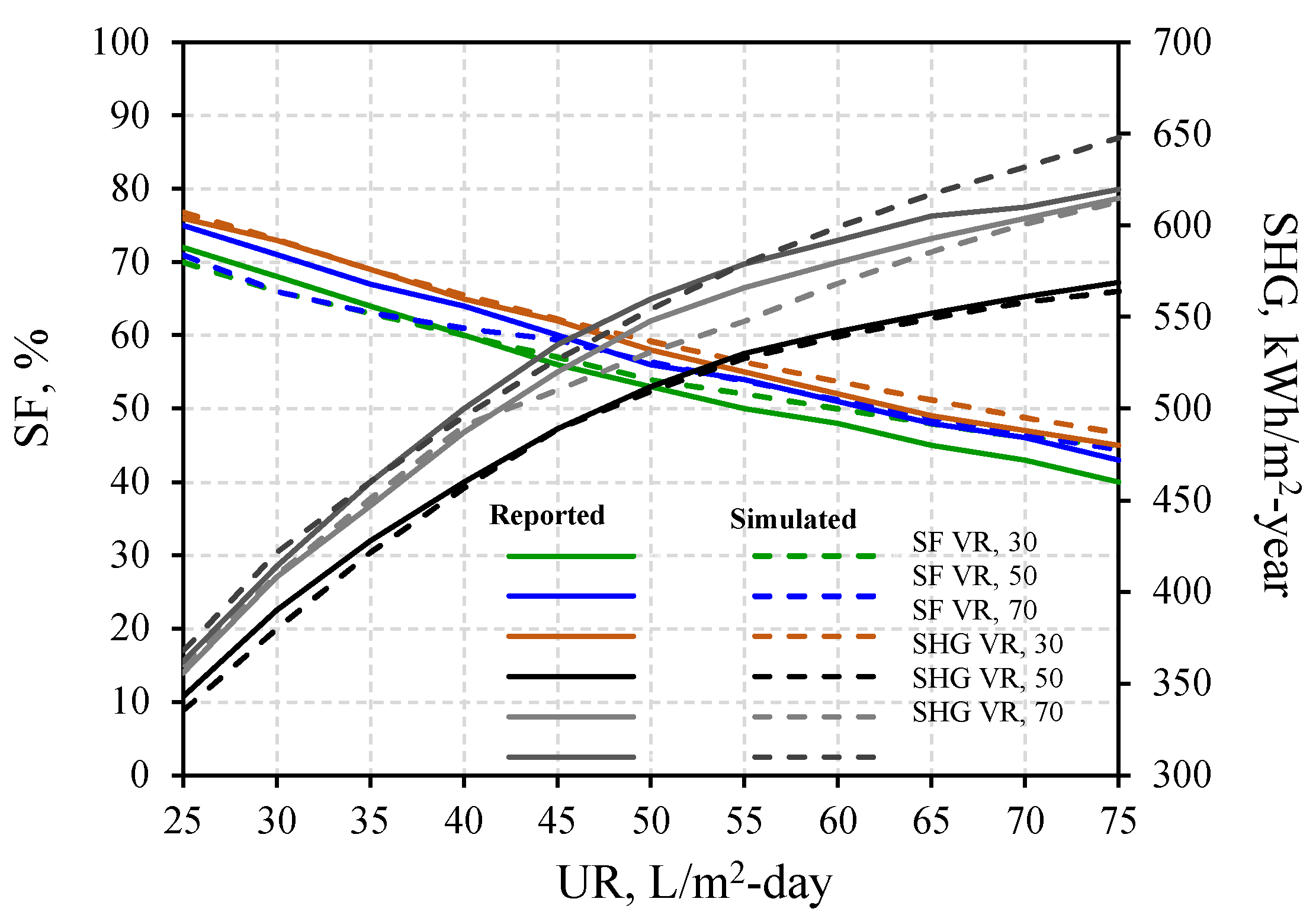
3.3.2. Utilization Ratio vs. Solar Fraction and Solar Heat Gain

Figure 10 compares the annual solar heating performance of SWHS-AHT (Figure 10a) and a conventional SWHS (Figure 10b) in terms of SF and SHG as a function of UR. Both systems achieved high SF in Saltillo, with SWHS-AHT reaching 99.6% and the conventional SWHS reaching 99.0%. However, the SWHS-AHT exhibited a more stable SF and SHG across a wider UR range (49 to 139 L/m²-day), with a significant increase in the rate of change observed beyond this point. Conversely, the conventional SWHS displayed a higher rate of change in both SF and SHG for all UR values. This behavior highlights the SWHS-AHT’s superior ability to utilize energy per unit collector area. The SWHS-AHT achieved a SHG of 569.2 kWh/m²-year with a collector area of 350 m² (UR of 49 L/m²-day) and 1352.0 kWh/m²-year with a collector area of 50 m² (UR of 345.6 L/m²-day). In contrast, the conventional SWHS achieved a SHG of 127.0 kWh/m²-year with a collector area of 650 m² (UR of 2.6 L/m²-day) and 811.9 kWh/m²-year with a collector area of 50 m² (UR of 33.9 L/m²-day). Similar trends were observed in Toluca and Tapachula, with the SWHS-AHT consistently achieving higher SF and SHG compared to the conventional SWHS. Notably, the SWHS-AHT performance remained relatively stable for UR values up to a specific point, demonstrating its ability to handle varying hot water demands.

3.3.3. Net Solar Collector Area vs. Auxiliary Heat and Solar Fraction

Figure 11 compares the annual solar heating performance of SWHS-AHT (Figure 11a) and a conventional SWHS (Figure 11b) in terms of Q_aux and SF as a function of A_c. The results are presented for three Mexican cities: Saltillo, Toluca, and Tapachula. In all cities, SWHS-AHT displayed a significant reduction in required A_c compared to the SWHS while achieving similar or slightly higher Q_aux and SF. For example, in Saltillo, an SWHS-AHT with 130 m² of A_c achieved a performance comparable to an SWHS with 300 m² of A_c, with a potential investment cost saving of €65,365.0 (based on an average cost of €384.5/m² from Table 1). This difference is attributed to the superior solar heat utilization of the SWHS-AHT system. Similar trends were observed in Toluca and Tapachula, with SWHS-AHT requiring less A_c to achieve comparable performance to the SWHS. The specific reduction in A_c and potential cost savings varied depending on the city’s climate. Notably, Tapachula, with the warmest climate, allowed for the most significant A_c reduction (225 m²), translating to potential savings of €86,512.5. These findings demonstrate the potential of SWHS-AHT technology to reduce the footprint and investment costs of solar water heating systems in various climatic conditions while maintaining high performance.

3.3.4. Net Solar Collector Area vs. Storage Tank Volume and Auxiliary Heat

Figure 12 compares the annual solar heating performances of the SWHS-AHT (Figure 12a) and SWHS (Figure 12b) in terms of V_t and Q_aux as a function of A_c. In Saltillo, for a target Q_aux of 1301.7 kW-year, the SWHS-AHT achieved this with a smaller A_c (130 m²) and V_t (15.6 m³) compared to the conventional SWHS (A_c: 300 m², V_t: 12.0 m³). The conventional SWHS achieved a slightly higher Q_aux (1317.9 kW-year). Similarly, in Toluca, the SWHS-AHT achieved a Q_aux of 1252.6 kW-year with a lower A_c (250 m²) and higher V_t (24.0 m³) compared to the conventional SWHS (A_c: 438 m², V_t: 17.5 m³). Both systems achieved the same target Q_aux in this case. Finally, in Tapachula, the SWHS-AHT achieved the target Q_aux of 1106.4 kW-year with a significantly reduced A_c (150 m²) and comparable V_t (18.0 m³) compared to the conventional SWHS (A_c: 375 m², V_t: 15.0 m³).

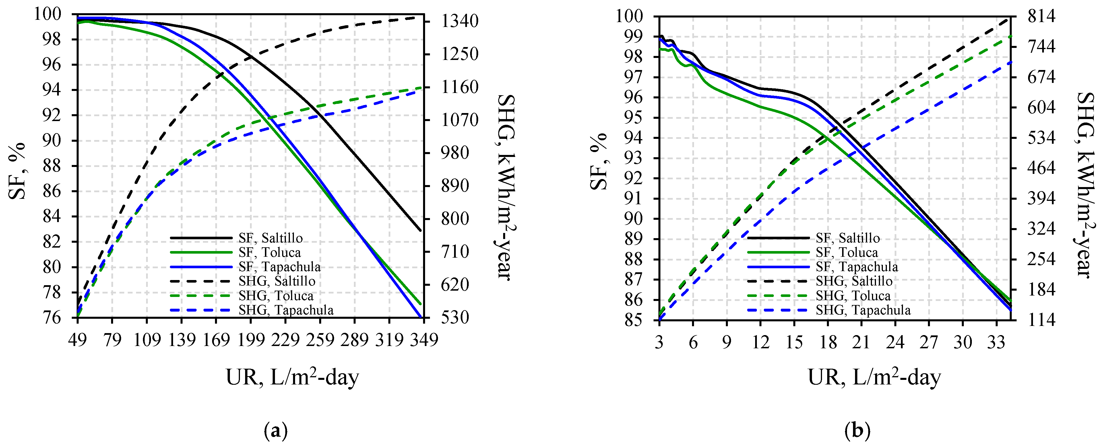
3.4. Annual Performance of the SWHS-AHT System

Figure 13 compares the annual average absorber useful heat water temperature (T8) and COP achieved by the SWHS-AHT system for different locations: Saltillo (Figure 13a), Toluca (Figure 13b), and Tapachula (Figure 13c). In each case, a specific SWHS-AHT configuration was selected to meet the established thermal requirements. For Saltillo, a system with an A_c of 130 m² and V_t of 15.6 m³ was employed. In Toluca, A_c and V_t were 250 m² and 24 m³, respectively, and in Tapachula, 150 m² and 18 m³. The SWHS-AHT successfully achieved the desired thermal conditions in all locations. The system consistently increased the water temperature from 15.8 °C to 94.4 °C, utilizing 81.2 °C heating water. On average, T8 was 12.9 °C higher than T1, and the average COP reached 0.44.

4. Conclusions

The performance assessment of solar heating through a coupled SWHS-AHT system for annual continuous water heating in three Mexican cities (Saltillo, Toluca, and Tapachula) demonstrated its potential as a more efficient solution compared to conventional SWHS. The SWHS-AHT system achieved higher SF and SHG while maintaining the same Q_aux. Additionally, it required a lower A_c and V_t, offering improved performance and reduced footprint. The conclusions of this work were as follows:

• The SWHS-AHT achieved a minimal variation in SF compared to the conventional SWHS in all cities. The SWHS-AHT reached an SF of 99.6% compared to 99.0% for the conventional SWHS.
• The SWHS-AHT delivered superior SHG compared to the conventional SWHS in all cities. The SWHS-AHT achieved a maximum SHG of 1352.0 kWh/m²-year with a collector area of 50 m², whereas the conventional SWHS reached a maximum SHG of 811.9 kWh/m²-year with the same A_c.
• The SWHS-AHT required a significantly smaller A_c to achieve a comparable Q_aux compared to the conventional SWHS. This reduction ranged from 42.9 to 60%. For instance, in Saltillo, the SWHS-AHT achieved a Q_aux of 1301.7 kW-year with an A_c of 130 m², while the conventional SWHS required an A_c of 300 m² for a slightly higher Q_aux of 1317.9 kW-year. This translates to potential cost savings due to a reduced number of solar collectors needed for the SWHS-AHT system. Optimal SWHS-AHT configurations achieved target Q_aux values with UR ranging from 49.4 to 345.6 L/m²-day and VR of 120 L/m² while utilizing mass flow rates of 1.38 kg/s. In contrast, conventional SWHS configurations required UR from 3 to 33.8 L/m²-day, VR of 40 L/m², and lower mass flow rates of 0.972 kg/s for comparable performance.
• The V_t exhibited a linear relationship with the A_c for both systems. However, the SWHS-AHT achieved a comparable V_t to the conventional SWHS despite requiring a smaller A_c.
• The SWHS-AHT demonstrated activation performance comparable to the findings of Varela-Martinez et al. by maintaining a GTL of 12.9 °C and a COP of 0.44 throughout the year. This improvement stemmed from the ANN’s effective monitoring of the AHT prototype temperatures.
• It is crucial to acknowledge that the SWHS-AHT configurations exhibiting the highest performance in this study demanded high SF values, ranging from 99.0% to 99.6%.
• Tracking the predicted variables reveals consistent quality of fit across all cases, with an average R² of 0.964 and an average MAE of 2.7 °C for the 12 predicted temperatures. These results validate the effectiveness of the proposed system in various thermal conditions. The ability of the SWHS-AHT to maintain performance despite variations in heat sources is an important aspect of ensuring the continuous availability of hot water in any process that requires it.

References

1. Kumar, L.; Hasanuzzaman, M.; Rahim, N.A. Global Advancement of Solar Thermal Energy Technologies for Industrial Process Heat and Its Future Prospects: A Review. Energy Convers. Manag. 2019, 195, 885–908. [Google Scholar] [CrossRef]
2. Salgado-Conrado, L.; Lopez-Montelongo, A. Barriers and Solutions of Solar Water Heaters in Mexican Household. Sol. Energy 2019, 188, 831–838. [Google Scholar] [CrossRef]
3. McMillan, C.; Xi, W.; Zhang, J.; Masanet, E.; Kurup, P.; Schoeneberger, C.; Meyers, S.; Margolis, R. Evaluating the Economic Parity of Solar for Industrial Process Heat. Sol. Energy Adv. 2021, 1, 100011. [Google Scholar] [CrossRef]
4. Ritchie, H.; Rosado, P.; Roser, M. Energy. Available online: https://ourworldindata.org/energy (accessed on 23 November 2023).
5. Tuncer, A.D.; Aytaç, İ.; Variyenli, H.İ.; Khanlari, A.; Mantıcı, S.; Karartı, A. Improving the Performance of a Heat Pipe Evacuated Solar Water Collector Using a Magnetic NiFe2O4/Water Nanofluid. Therm. Sci. Eng. Prog. 2023, 45, 102107. [Google Scholar] [CrossRef]
6. Delgado-Gonzaga, J.; Juárez-Romero, D.; Saravanan, R.; Márquez-Nolasco, A.; Huicochea, A.; Morales, L.I. Performance Analysis of a Dual Component Generator-Condenser of an Absorption Heat Transformer for Water Desalination. Therm. Sci. Eng. Prog. 2020, 20, 100651. [Google Scholar] [CrossRef]
7. Rivera, W.; Best, R.; Cardoso, M.J.; Romero, R.J. A Review of Absorption Heat Transformers. Appl. Therm. Eng. 2015, 91, 654–670. [Google Scholar] [CrossRef]
8. Benli, H. Potential Application of Solar Water Heaters for Hot Water Production in Turkey. Renew. Sustain. Energy Rev. 2016, 54, 99–109. [Google Scholar] [CrossRef]
9. Jaisankar, S.; Ananth, J.; Thulasi, S.; Jayasuthakar, S.T.; Sheeba, K.N. A Comprehensive Review on Solar Water Heaters. Renew. Sustain. Energy Rev. 2011, 15, 3045–3050. [Google Scholar] [CrossRef]
10. Faisal Ahmed, S.; Khalid, M.; Vaka, M.; Walvekar, R.; Numan, A.; Khaliq Rasheed, A.; Mujawar Mubarak, N. Recent Progress in Solar Water Heaters and Solar Collectors: A Comprehensive Review. Therm. Sci. Eng. Prog. 2021, 25, 100981. [Google Scholar] [CrossRef]
11. Sabiha, M.A.; Saidur, R.; Hassani, S.; Said, Z.; Mekhilef, S. Energy Performance of an Evacuated Tube Solar Collector Using Single Walled Carbon Nanotubes Nanofluids. Energy Convers. Manag. 2015, 105, 1377–1388. [Google Scholar] [CrossRef]
12. Sharifi, S.; Nozad Heravi, F.; Shirmohammadi, R.; Ghasempour, R.; Petrakopoulou, F.; Romeo, L.M. Comprehensive Thermodynamic and Operational Optimization of a Solar-Assisted LiBr/Water Absorption Refrigeration System. Energy Rep. 2020, 6, 2309–2323. [Google Scholar] [CrossRef]
13. Al-Mamun, M.R.; Roy, H.; Islam, M.S.; Ali, M.R.; Hossain, M.I.; Saad Aly, M.A.; Hossain Khan, M.Z.; Marwani, H.M.; Islam, A.; Haque, E.; et al. State-of-the-Art in Solar Water Heating (SWH) Systems for Sustainable Solar Energy Utilization: A Comprehensive Review. Sol. Energy 2023, 264, 111998. [Google Scholar] [CrossRef]
14. Gautam, A.; Chamoli, S.; Kumar, A.; Singh, S. A Review on Technical Improvements, Economic Feasibility and World Scenario of Solar Water Heating System. Renew. Sustain. Energy Rev. 2017, 68, 541–562. [Google Scholar] [CrossRef]
15. SHIP Solar Heat for Industrial Processes. Available online: http://ship-plants.info/ (accessed on 28 May 2024).
16. Chopra, K.; Tyagi, V.V.; Pathak, S.K.; Sharma, R.K.; Mansor, M.; Goel, V.; Sari, A. 5E Analysis of a Novel Designed Hot Water Storage Header Integrated Vacuum Tube Solar Water Heater. Therm. Sci. Eng. Prog. 2023, 42, 101929. [Google Scholar] [CrossRef]
17. Lee, M.; Shin, Y.; Cho, H. Performance Evaluation of Flat Plate and Vacuum Tube Solar Collectors by Applying a MWCNT/Fe3O4 Binary Nanofluid. Energies 2020, 13, 1715. [Google Scholar] [CrossRef]
18. Ismail, K.A.R.; Teles, M.P.R.; Lino, F.A.M. Comparative Analysis of Eccentric Evacuated Tube Solar Collector with Circular and Rectangular Absorber Working with Nanofluid. Clean. Eng. Technol. 2021, 3, 100105. [Google Scholar] [CrossRef]
19. Duffie, J.A.; Beckman, W.A.; Worek, W.M. Solar Engineering of Thermal Processes, 4th ed.; Wiley: New York, NY, USA, 2003; Volume 116, 944p, ISBN 1118418123. [Google Scholar]
20. Ononogbo, C.; Nwosu, E.C.; Nwakuba, N.R.; Nwaji, G.N.; Nwufo, O.C.; Chukwuezie, O.C.; Chukwu, M.M.; Anyanwu, E.E. Opportunities of Waste Heat Recovery from Various Sources: Review of Technologies and Implementation. Heliyon 2023, 9, e13590. [Google Scholar] [CrossRef] [PubMed]
21. Mehrjouiee, H.; Fallah, M.; Mohammad, S.; Mahmoudi, S. Advanced Exergy Analysis of a Double Absorption Heat Transformer Recovering Industrial Waste Heat for Pure Water Production. Therm. Sci. Eng. Prog. 2024, 47, 102242. [Google Scholar] [CrossRef]
22. Liu, Z.; Lu, D.; Tao, S.; Chen, R.; Gong, M. Experimental Study on Using 85 °C Low-Grade Heat to Generate <120 °C Steam by a Temperature-Distributed Absorption Heat Transformer. Energy 2024, 299, 131491. [Google Scholar] [CrossRef]
23. Cudok, F.; Giannetti, N.; Ciganda, J.L.C.; Aoyama, J.; Babu, P.; Coronas, A.; Fujii, T.; Inoue, N.; Saito, K.; Yamaguchi, S.; et al. Absorption Heat Transformer-State-of-the-Art of Industrial Applications. Renew. Sustain. Energy Rev. 2021, 141, 110757. [Google Scholar] [CrossRef]
24. Perez, S.G.; Huicochea, A.; Urquiza, G.; Hernández, A.H.; Siqueiros, J. The Commissioning of Absorption Heat Transformer for Water Distillation Using Solar Panels. Desalin. Water Treat. 2020, 204, 1–11. [Google Scholar] [CrossRef]
25. Salata, F.; Coppi, M. A First Approach Study on the Desalination of Sea Water Using Heat Transformers Powered by Solar Ponds. Appl. Energy 2014, 136, 611–618. [Google Scholar] [CrossRef]
26. Gomri, R. Energy and Exergy Analyses of Seawater Desalination System Integrated in a Solar Heat Transformer. Desalination 2009, 249, 188–196. [Google Scholar] [CrossRef]
27. Wang, J.; Chen, H.; Deng, H.; Dong, F. A Combined Power and Steam System Integrated with Solar Photovoltaic/Thermal Collector: Thermodynamic Characteristics and Cost-Benefit Analyses. Case Stud. Therm. Eng. 2022, 39, 102477. [Google Scholar] [CrossRef]
28. Wang, H.; Li, H.; Wang, L.; Bu, X.; Zeng, J.; Xie, N.; Xu, Q. A Solar-Assisted Double Absorption Heat Transformer: Off-Design Performance and Optimum Control Strategy. Energy Convers. Manag. 2019, 196, 614–622. [Google Scholar] [CrossRef]
29. Liu, F.; Sui, J.; Liu, T.; Jin, H. Energy and Exergy Analysis in Typical Days of a Steam Generation System with Gas Boiler Hybrid Solar-Assisted Absorption Heat Transformer. Appl. Therm. Eng. 2017, 115, 715–725. [Google Scholar] [CrossRef]
30. Chaiyat, N.; Kiatsiriroat, T. Simulation and Experimental Study of Solar-Absorption Heat Transformer Integrating with Two-Stage High Temperature Vapor Compression Heat Pump. Case Stud. Therm. Eng. 2014, 4, 166–174. [Google Scholar] [CrossRef]
31. INEGI Instituto Nacional de Estadística y Geografía. Available online: https://www.inegi.org.mx/app/areasgeograficas/#collapse-Resumen (accessed on 21 May 2024).
32. SENER Secretaria de Energía. Available online: https://www.gob.mx/sener (accessed on 21 May 2024).
33. SMN Servicio Meteorologico Nacional. Available online: https://smn.conagua.gob.mx/es/ (accessed on 23 November 2023).
34. Heß, S.; Oliva, A. Guide to Solar Thermal System Design for Selected Industrial Processes; O. Ö. Energiesparverband: Linz, Austria, 2010. [Google Scholar]
35. Duffie, J.; Beckman, W.; Worek, W.M. Solar Engineering of Thermal Processes, 2nd ed.; Wiley: New York, NY, USA, 1991; 919p. [Google Scholar]
36. winsconsin University TRNSYS 16.1. Available online: https://sel.me.wisc.edu/trnsys/features/ (accessed on 2 June 2019).
37. Kalogirou, S.A. Designing and Modeling Solar Energy Systems. In Solar Energy Engineering; Elsevier: Amsterdam, The Netherlands, 2014; pp. 583–699. [Google Scholar] [CrossRef]
38. Tamhane, A.C. Single Factor Experiments: Completely Randomized Designs. In Statistical Analysis of Designed Experiments; John Wiley & Sons, Inc.: Hoboken, NJ, USA, 2009; pp. 70–125. ISBN 9781118491621. [Google Scholar]
39. López-Pérez, L.A.; Flores-Prieto, J.; Ríos-Rojas, C. Comfort Temperature Prediction According to Adaptive Approach for Educational Buildings in Tropical Climate Using Artificial Neural Networks. Energy Build. 2021, 251, 111328. [Google Scholar] [CrossRef]
40. Tian, Z.; Perers, B.; Furbo, S.; Fan, J. Annual Measured and Simulated Thermal Performance Analysis of a Hybrid Solar District Heating Plant with Flat Plate Collectors and Parabolic Trough Collectors in Series. Appl. Energy 2017, 205, 417–427. [Google Scholar] [CrossRef]
41. Hernández, J.A.; Bassam, A.; Siqueiros, J.; Juárez-Romero, D. Optimum Operating Conditions for a Water Purification Process Integrated to a Heat Transformer with Energy Recycling Using Neural Network Inverse. Renew. Energy 2009, 34, 1084–1091. [Google Scholar] [CrossRef]
42. Solís-Pérez, J.E.; Gómez-Aguilar, J.F.; Hernández, J.A.; Escobar-Jiménez, R.F.; Viera-Martin, E.; Conde-Gutiérrez, R.A.; Cruz-Jacobo, U. Global Optimization Algorithms Applied to Solve a Multi-Variable Inverse Artificial Neural Network to Improve the Performance of an Absorption Heat Transformer with Energy Recycling. Appl. Soft Comput. J. 2019, 85, 105801. [Google Scholar] [CrossRef]
43. Morales, L.I.; Conde-Gutiérrez, R.A.; Hernández, J.A.; Huicochea, A.; Juárez-Romero, D.; Siqueiros, J. Optimization of an Absorption Heat Transformer with Two-Duplex Components Using Inverse Neural Network and Solved by Genetic Algorithm. Appl. Therm. Eng. 2015, 85, 322–333. [Google Scholar] [CrossRef]
44. Varela-Martínez, K.; Hernández, J.A.; Juárez, D.; Huicochea, A. Heat Transfer Study of Four Nested Helical Coils inside an Absorption Heat Transformer. Exp. Heat Transf. 2022, 35, 993–1015. [Google Scholar] [CrossRef]
45. MathWorks Inc. Statistics and Machine Learning ToolboxTM User’s Guide. 1993. Available online: http://cda.psych.uiuc.edu/matlab_pdf/stats.pdf (accessed on 28 May 2024).
46. Delgado-Gonzaga, J.; Rivera, W.; Juárez-Romero, D. Integration of Cycles by Absorption for the Production of Desalinated Water and Cooling. Appl. Therm. Eng. 2023, 220, 119718. [Google Scholar] [CrossRef]
47. Demesa, N.; Hernández, J.A.; Juárez, D.; Huicochea, A. Experimental Assessment of Heat Exchangers with Nested Helical Coils for an Absorption Heat Transformer. Exp. Heat Transf. 2021, 34, 140–161. [Google Scholar] [CrossRef]
48. Bern, C.; Huguenin-landl, B.; Studer, C. Handbook Part I: Software Global Meteorological Database Version 7 Software and Data for Engineers, Planers and Education. 2017. Available online: https://meteonorm.com/assets/downloads/mn73_software.pdf (accessed on 13 April 2024).
49. Deng, Z.; Chen, Q. Artificial Neural Network Models Using Thermal Sensations and Occupants’ Behavior for Predicting Thermal Comfort. Energy Build. 2018, 174, 587–602. [Google Scholar] [CrossRef]
Figure 1. Study method.
Processes 12 01650 g001
Figure 2. Solar resources in testing places.
Processes 12 01650 g002
Figure 3. Schematic representation of the main components of the simulated solar water heating system.
Processes 12 01650 g003
Figure 4. Piping and instrumentation diagram of the AHT prototype.
Processes 12 01650 g004
Figure 5. Flow diagram for calculating the heat fluxes and COP of the AHT-ANN model.
Processes 12 01650 g005
Figure 6. TRNSYS simulation platform for SWHS and SWHS-AHT systems.
Processes 12 01650 g006
Figure 7. Comparison of simulated SWHS and theoretical SWHS performance.
Processes 12 01650 g007
Figure 8. Schematic representation of the optimized ANN-BM model.
Processes 12 01650 g008
Figure 9. Comparative of the temperatures predicted by the optimized AHT-ANN model and the target temperatures.
Processes 12 01650 g009aProcesses 12 01650 g009b
Figure 10. Comparison of Utilization Ratio vs. Solar Fraction and Solar Heat Gain for SWHS-AHT (a) and conventional SWHS (b).
Processes 12 01650 g010
Figure 11. Comparison of Net Collector Area vs. Auxiliary Heat and Solar Fraction for SWHS-AHT (a) and conventional SWHS (b).
Processes 12 01650 g011
Figure 12. Comparison of Net collector area vs. Storage tank volume and Auxiliary heat for SWHS-AHT (a) and conventional SWHS (b).
Processes 12 01650 g012
Figure 13. Performance of SWHS-AHT in Saltillo (a), Toluca (b), and Tapachula (c) in terms of temperatures and Coefficient of Performance.
Processes 12 01650 g013