Dynamic Evolution Law of Production Stress Field in Fractured Tight Sandstone Horizontal Wells Considering Stress Sensitivity of Multiple Media

Abstract

Inter-well frac-hit has become an important challenge in the development of unconventional oil and gas resources such as fractured tight sandstone. Due to the presence of hydraulic fracturing fractures, secondary induced fractures, natural fractures, and other seepage media in real formations, the acquisition of stress fields requires the coupling effect of seepage and stress. In this process, there is also stress sensitivity, which leads to unclear dynamic evolution laws of stress fields and increases the difficulty of the staged multi-cluster fracturing of horizontal wells. The use of a multi-stage stress-sensitive horizontal well production stress field prediction model is an effective means of analyzing the influence of natural fracture parameters, main fracture parameters, and multi-stage stress sensitivity coefficients on the stress field. This article considers multi-stage stress sensitivity and, based on fractured sandstone reservoir parameters, establishes a numerical model for the dynamic evolution of the production stress field in horizontal wells with matrix self-supporting fracture-supported fracture–seepage–stress coupling. The influence of various factors on the production stress field is analyzed. The results show that under constant pressure production, for low-permeability reservoirs, multi-stage stress sensitivity has a relatively low impact on reservoir stress, and the amplitude of principal stress change in the entire fracture length direction is only within the range of 0.27%, with no significant change in stress distribution; The parameters of the main fracture have a significant impact on the stress field, with a variation amplitude of within 2.85%. The ability of stress to diffuse from the fracture tip to the surrounding areas is stronger, and the stress concentration area spreads from an elliptical distribution to a semi-circular distribution. The random natural fracture parameters have a significant impact on pore pressure. As the density and angle of the fractures increase, the pore pressure changes within the range of 3.32%, and the diffusion area of pore pressure significantly increases, making it easy to communicate with the reservoir on both sides of the fractures.

1. Introduction

Tight sandstone gas is widely present in major oil and gas basins around the world, becoming one of the important unconventional gas types. With the breakthrough of reservoir simulation technology and the decrease in development costs, the scale and industrial development of tight sandstone gas have been promoted. China is the third largest producer of tight sandstone gas in the world, and by 2020, the annual production of tight sandstone gas has reached 470 × 10⁸ m³ [1]. However, tight sandstone reservoirs have characteristics such as low porosity and low permeability, making their extraction difficult. The combination of horizontal well drilling and large-scale hydraulic fracturing technology can achieve efficient and cost-effective development of tight sandstone gas. The complex fracture network formed by large-scale hydraulic fracturing provides flow channels for oil and gas seepage [2,3]. Due to the development of natural fractures and the presence of complex fracture networks, the distance between development wells continues to shrink, and the fracturing connection between adjacent wells on multiple well platforms causes inter-well interference. That is, when a well is fractured, it is connected to adjacent wells, resulting in a sudden and significant increase in fluid production, an increase in casing pressure, and a significant decrease in gas production [4]. For example, 80% of the wells in a fractured tight sandstone reservoir are affected, and the gas production is more than 80%. It is difficult to recover the initial gas production from pressure wells, and only 38% of frac-hit wells can recover to more than 50% of the gas production before pressure wells [5]. On the one hand, inter-well frac-hit affects the production performance of production wells and reduces production capacity. On the other hand, artificial fractures communicating with low-pressure areas are not conducive to maintaining net pressure in fractured wells, which affects the effectiveness of transformation. The presence of inter-well frac-hit is the problem of fracture propagation and connectivity between different wells. In order to effectively reduce the occurrence of inter-well pressure channeling, it is necessary to have a clear understanding of the production stress field state of the parent well and provide support for the analysis of new fracture propagation.

Numerous scholars have conducted research on the distribution pattern and influencing factors of stress field around hydraulic fracturing fractures, mainly including experimental, theoretical, and numerical studies. In 2008, He et al. [6] constructed a laboratory instrument to simulate fluid injection programs and the three-dimensional stress field around test samples. In 2010, M G. Mack, Bruno, and Nakagawab et al. pointed out that after a hydraulic fracturing transformation, a new induced stress will form in the direction perpendicular to the fracture in the formation. The presence of induced stress may cause changes in the geostress around the wellbore, and after further fracturing, new fractures will turn in the direction of induced stress [7]. In 2018, Mortazavi [8] applied a newly designed true triaxial stress loading and pore pressure application device (TTSL-PPAA) to study the coupling between pore pressure reduction and reservoir stress changes under actual field conditions by reducing pore pressure and simulating pore pressure reduction under constant vertical and zero horizontal strain (i.e., uniaxial strain boundary conditions). The indoor experiment has preliminarily revealed the law of stress variation but can only provide some qualitative understanding. It is limited by the equipment scale and pressure capacity, and the experimental parameters greatly differ from the field, which has limited guiding significance for practical engineering applications.

Therefore, many scholars have also calculated and analyzed the stress field from the perspective of theoretical solutions. Currently, there are mainly analytical, semi-analytical, and numerical methods for calculating induced stress fields. Sneddon and Elliott [9,10] derived analytical models of stress fields around flat fractures and infinitely long fractures and obtained analytical solutions; Palmer [11] analyzed the induced stress field generated by first fracturing in coalbed methane reservoirs, proposed that induced stress can induce stress deflection near the fractures, and discussed the effects of fracture morphology and net fracture pressure on reservoir permeability; Zhai [12] et al. established a pore elasticity model and obtained its analytical solution, which describes the expression of the relationship between porous elastic stress and horizontal minimum and maximum principal stresses, pore pressure, and wellbore radius. Based on the principle of stress superposition, Li [13] simplified the physical quantity relationship of traditional induced stress models, derived a mathematical model of horizontal induced stress difference for multiple fracture superposition, and analyzed the single factor variation law that affects the induced stress difference of fractures. The stress field analytical model established in a two-dimensional plane is simple to calculate, but the analytical formula is derived based on certain assumptions, which has a significant deviation from the actual situation.

In contrast, numerical methods have more advantages in analyzing the stress field of actual geological formations. Li [14] et al. conducted quantitative characterization research on three-dimensional hydraulic fracturing fractures; Erhu Liu [15] combined the boundary element method and the maximum circumferential tensile stress criterion to establish a numerical model that can simulate the development of fracturing fractures and stress fields. The accuracy of the model was verified using analytical solutions. The model was used to analyze the expansion of horizontal well filled fracturing fractures under different conditions; B. Moradi Bajestani [16,17] et al. analyzed hydraulic fractures through a series of fluid dynamics coupled simulations and studied the effects of rock mechanics and geometric properties, injection rate, natural fractures, and other parameters on hydraulic fracture propagation; Jaber Taheri Shakib [18] conducted numerical simulations of hydraulic fracturing by considering the influence of stress on the interaction between hydraulic fractures and parallel natural fractures; Li [19] et al. studied the redistribution of stress and fracture propagation during the process of shale gas reservoir stimulation; Saberhosseini, SE [20] et al. prepared a fully coupled stress diffusion XFEM model for the occurrence and propagation of multiple hydraulic fractures in five injection zones to optimize the effects of fracture spacing and pore pressure changes on the deviation and geometric shape of multiple hydraulic fractures.

Overall, most studies on stress fields solely focus on factors such as fracture parameters and fluid properties. However, in real geological formations, there are often multiple seepage media such as hydraulic fracturing fractures, secondary fractures, and natural fractures. The acquisition of stress fields requires coupling of seepage and stress, and in this process, factors such as permeability are stress sensitive. The changes in stress fields when these three factors are simultaneously considered are not yet clear. Therefore, this article considers multi-stage stress sensitivity and, based on the parameters of fractured tight sandstone reservoirs, establishes a numerical model for the dynamic evolution of the stress field coupled with matrix self-supporting fractures supporting fractures–seepage–stress coupling. The influence of various factors on the production stress field is analyzed, and the research results are helpful for analyzing the changes in the stress field around the production well.

2. Model Establishment

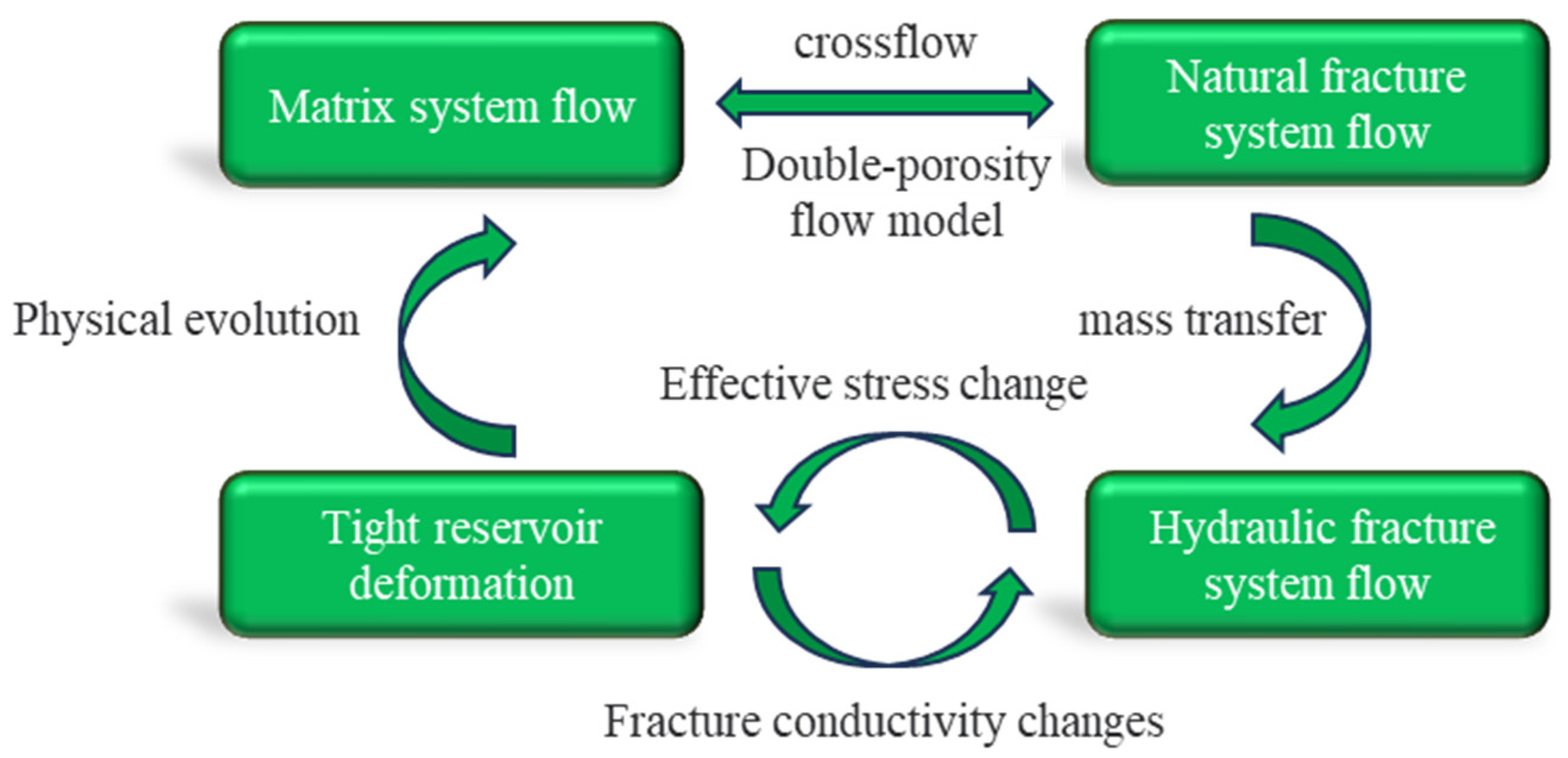
2.1. Physical Model

In the process of oil and gas reservoir development, the seepage field and the stress field are a bidirectional coupling process. The seepage of fluids leads to changes in the pore pressure of the formation, resulting in changes in the effective stress on the reservoir rocks and deformation of the rocks. At the same time, the deformation of reservoir rocks also affects the changes in reservoir pore volume, thereby affecting the characteristics of seepage. The elastic theory of porous media and the mechanism of fluid solid coupling are shown in Figure 1. The basic assumptions of this model are as follows: ① The reservoir is composed of a matrix system and a natural fracture system, with a quasi-steady-state flow between the two. ② A porous medium is considered as a fully saturated and isotropic linear elastic body. ③ The reservoir undergoes elastic deformation, satisfying the assumption of small deformation and following the Terzaghi effective stress principle. ④ The isothermal flow of single-phase fluid follows Darcy’s law, ignoring the influence of gravity. ⑤ Crude oil flows from the matrix system through natural fractures toward fractured fractures and wellbore.

2.2. Mathematical Models

The model in this article considers the stress sensitivity coefficient, and each parameter is not a constant value in the production process, but a variable that varies with the effective stress. The specific expression is as follows:

Permeability stress-sensitive equation

$$k_{rock}=k_0{\left({\displaystyle \frac{p_e}{p_0}}\right)}^{s_k}$$

(1)

where $k_{rock}$ is the matrix permeability, $k_0$ is the initial matrix permeability, $p_0$ is the atmospheric pressure, $p_e$ is the effective stress, and $s_k$ is the permeability stress sensitivity coefficient, $s_k$ < 1.

$$k_f=k_{f0}{e}^{-3c_f({\sigma }_e-{\sigma }_{e0})}$$

(2)

where $k_f$ is the crack permeability, $k_{f0}$ is the initial crack permeability, ${\sigma }_e$ is the effective stress on the crack wall, ${\sigma }_{e0}$ is the initial effective stress on the crack wall, and $c_f$ is the crack compression coefficient.

Stress-sensitive equation for porosity

$${\varphi }_{rock}={\varphi }_0{\left({\displaystyle \frac{p_e}{p_0}}\right)}^{s_{\varphi }}$$

(3)

where ${\varphi }_{rock}$ is the matrix porosity, ${\varphi }_0$ is the initial porosity of the matrix, and $s_{\varphi }$ is the porosity sensitivity coefficient.

Compression coefficient of fracture:

$$C_f={\displaystyle \frac{-1}{p_k\ln (p_k/p_h)}}$$

(4)

where $C_f$ is the compression coefficient of fracture, $p_k$ is the net fracture pressure, and $p_h$ is the recovery pressure (or standard stress state).

The mathematical model in this article includes the stress balance equation, the stress–strain geometric equation for reservoir rock deformation, the constitutive equation for controlling seepage–stress coupling, and the continuity equation for unidirectional fluid flow. The establishment and solution process of the mathematical model in this article can be found in Mu [21,22].

2.3. Finite Element Numerical Model

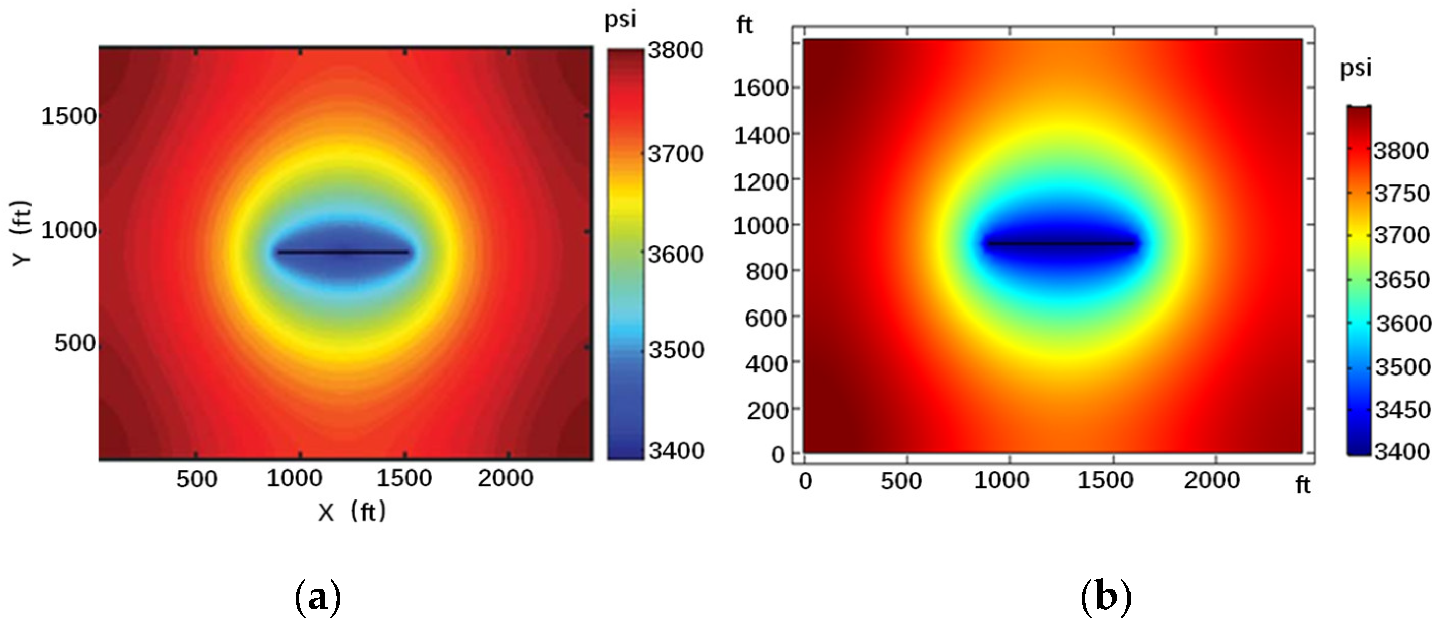
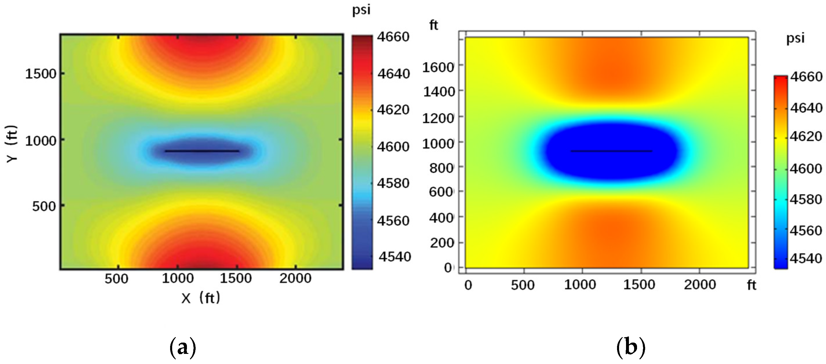
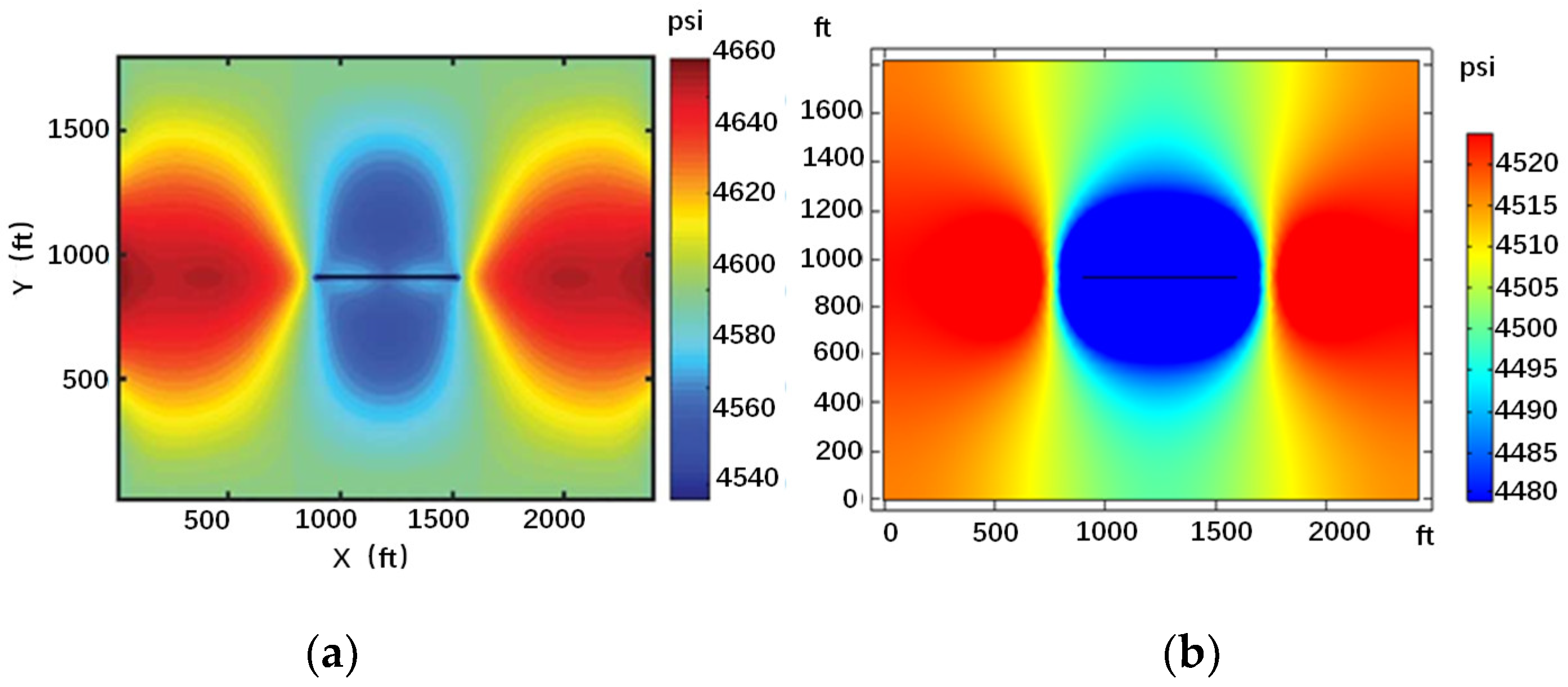
This article takes fractured tight sandstone reservoirs as the research object and establishes a geological numerical model of the target block (Figure 2). The model size is 200 m × 300 m, and the half-length of the fracture is 120 m. The y direction represents the maximum horizontal principal stress direction, and the x direction represents the minimum horizontal principal stress direction. The rock mechanics parameters and input parameters such as geostress are shown in

Table 1. Simulation Parameters Table.

Basic Parameter	Value
Initial matrix permeability (mD)	50
Poisson’s ratio	0.22
Bottom-hole pressure (MPa)	47
Original formation pressure (MPa)	57
Cluster count	5
Primary fracture length (m)	120
Primary fracture initial conductivity (Dc.cm)	1
Primary fracture compressibility coefficient (1/Pa)	8.00 × 10−9
Number of secondary fractures	8
Secondary fractures initial conductivity (Dc.cm)	0.1
Secondary fractures compressibility coefficient (1/Pa)	3.00 × 10−8
Compressibility coefficient (GPa)	21
Biot coefficient	0.7
Maximum horizontal principal stress (MPa)	83.8
Minimum horizontal principal stress (MPa)	70

.

3. Model Validation

Due to the fact that the stress seepage multifield coupling equation system not only considers the bidirectional coupling effect between different physical fields but also changes with time, it has typical nonlinearity and cannot be solved analytically. Therefore, this process uses finite-element numerical method to solve. There is currently no precise analytical solution to describe the relationship between pore pressure and stress caused by the fluid structure coupling effect. Therefore, in order to verify the reliability of the model in simulating the induced stress field caused by changes in pore pressure, taking a single crack in the production process as an example, this model is compared and verified with the results obtained by Anusarn Sangnimnuan and Wu Kan in 2018 by combining the fluid flow/geomechanics coupling model of EDFM. The model size is 737.6 m × 554.7 m, and the half-length of the crack is 106.7 m (Figure 3, Figure 4 and Figure 5).

From the graph, it can be seen that as production progresses, pressure waves continuously propagate outward, causing a decrease in stress in both the maximum and minimum horizontal principal stress directions around the crack. The stress in the maximum horizontal principal stress direction at the upper and lower ends of the crack increases, while the stress in the minimum horizontal principal stress direction at the left and right ends of the crack increases. By comparing the model in this article with the validation model, it can be seen that both the range of influence of the disturbed stress field and the numerical value of the disturbed stress field are basically consistent with the validation model. Therefore, it can be seen that the model established in this article can accurately simulate the induced stress field caused by changes in pore pressure. Figure 5. Comparison of stress in the direction of minimum horizontal principal stress.

4. Analysis of Impact Patterns

Quantify the trend of stress field changes by setting detection lines A–A′ and monitoring points B (80, 10) in the model, and then analyze the degree of influence of different factors on the stress field.

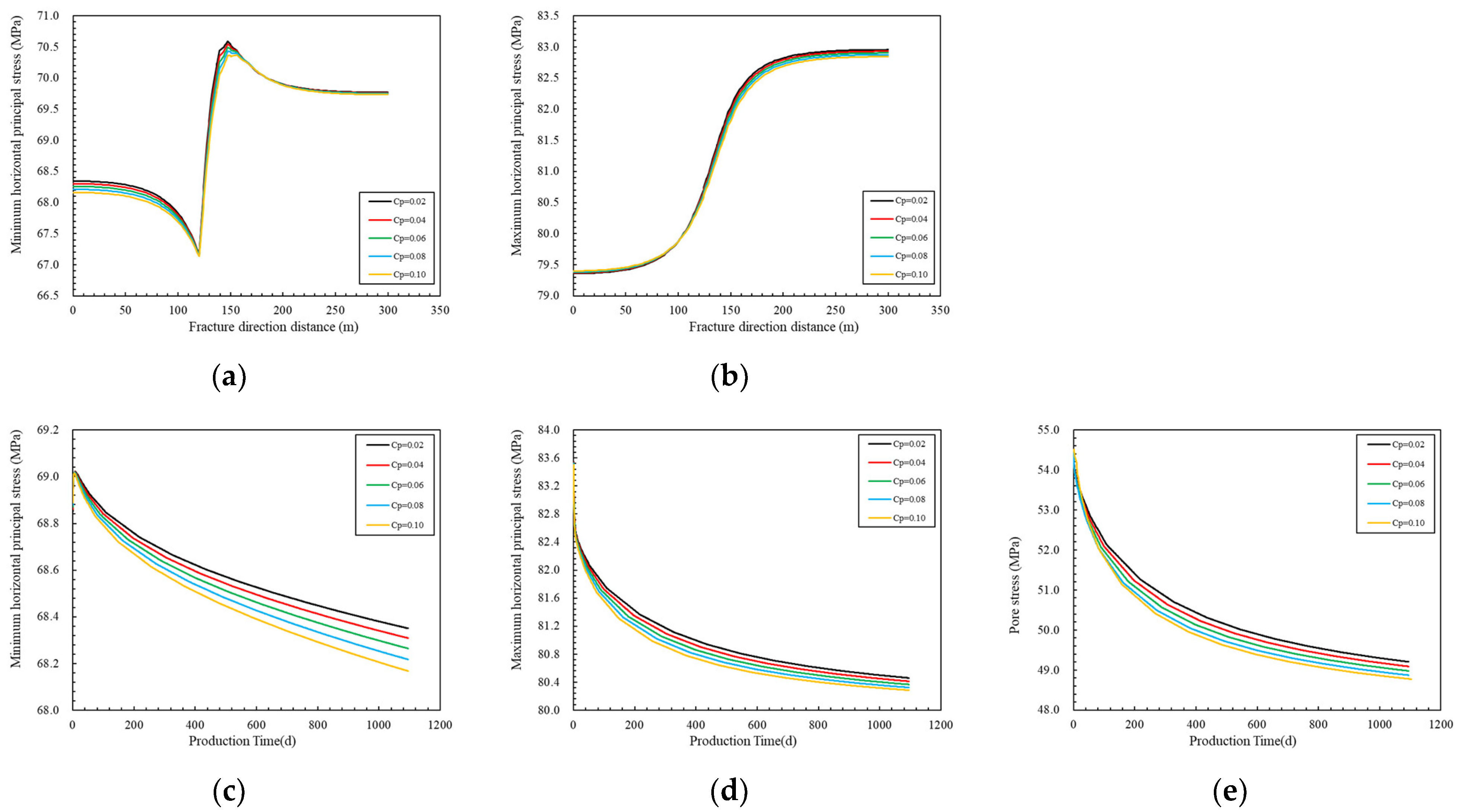
4.1. Stress Sensitivity Coefficient of Matrix Porosity

From Figure 6a,b, it can be observed that along the direction of the fracture, the minimum horizontal principal stress shows a decreasing trend in the fracture area, followed by the formation of a stress concentration zone at the tip of the fracture, and finally the formation stress level is restored. The maximum principal stress has been showing an upward trend. As the stress sensitivity coefficient of matrix porosity increases, the minimum horizontal principal stress value in the entire fracture length direction decreases, but the amplitude is small, only 0.27%. The maximum horizontal principal stress increases with the increase in the matrix porosity stress sensitivity coefficient before 120 m (in the fracture area) and reverses after 120 m and decreases with the increase in the matrix porosity stress sensitivity coefficient, with a greater impact than in the fracture area. From Figure 6c–e, it can be seen that both the principal stress and pore pressure show a decreasing trend, with the largest decrease in the early stage of production. As production progresses, the stress curve gradually flattens. After 3 years of production, the maximum horizontal principal stress decreased by 3.19–3.36 MPa, the minimum horizontal principal stress decreased by 1.55–1.64 MPa, and the pore pressure decreased by 7.35–7.61 MPa. Moreover, the larger the stress sensitivity coefficient of the matrix porosity, the greater the stress reduction. From the minimum horizontal principal stress cloud map in Figure 7, it can be observed that as the sensitivity coefficient of matrix porosity increases, the low stress zone spreads from the fracture finger to the fracture root, while the range of the high stress zone at the tip decreases, and the stress distribution shape remains unchanged. With the increase in the porosity sensitivity coefficient, the stability of cracks in rocks decreases, and cracks are more likely to expand under lower stress conditions. The spread of the crack will lead to the redistribution of the stress around it, but this redistribution will not change the overall shape of the stress field; it will only change the distribution of the stress.

4.2. Matrix Permeability Stress Sensitivity Coefficient

From Figure 8, it can be observed that along the direction of the fracture, as the stress sensitivity coefficient of the matrix permeability increases, the minimum horizontal principal stress shows an increasing trend, while the maximum horizontal principal stress first decreases and then increases. The impact trend is opposite to the stress sensitivity coefficient of the matrix porosity. The opposite reason is that with the increase in the stress sensitivity coefficient of matrix porosity, the matrix porosity will decrease, and the amount of oil and gas resources per unit space will be less. With the production progress, the stress sweep range will increase, resulting in a faster stress drop. With the increase in the matrix permeability stress sensitivity coefficient, matrix permeability will decrease; when the fluid flow is slower, and with the progress of production, the stress sweep range will decrease, resulting in a slower and lower stress drop. Within the entire region, the stress variation is within the range of 0.27%, and the degree of influence is similar to the stress sensitivity coefficient of matrix porosity. After 3 years of production, the stress reduction in the minimum principal stress was relatively small. Within 1.53–1.72 MPa, the maximum horizontal principal stress decreased by 3.19–3.36 MPa, and the pore pressure decreased by 7.31–7.75 MPa. Overall, the sensitivity coefficient of matrix permeability has a greater impact on pore pressure and a minimum impact on the maximum horizontal principal stress.

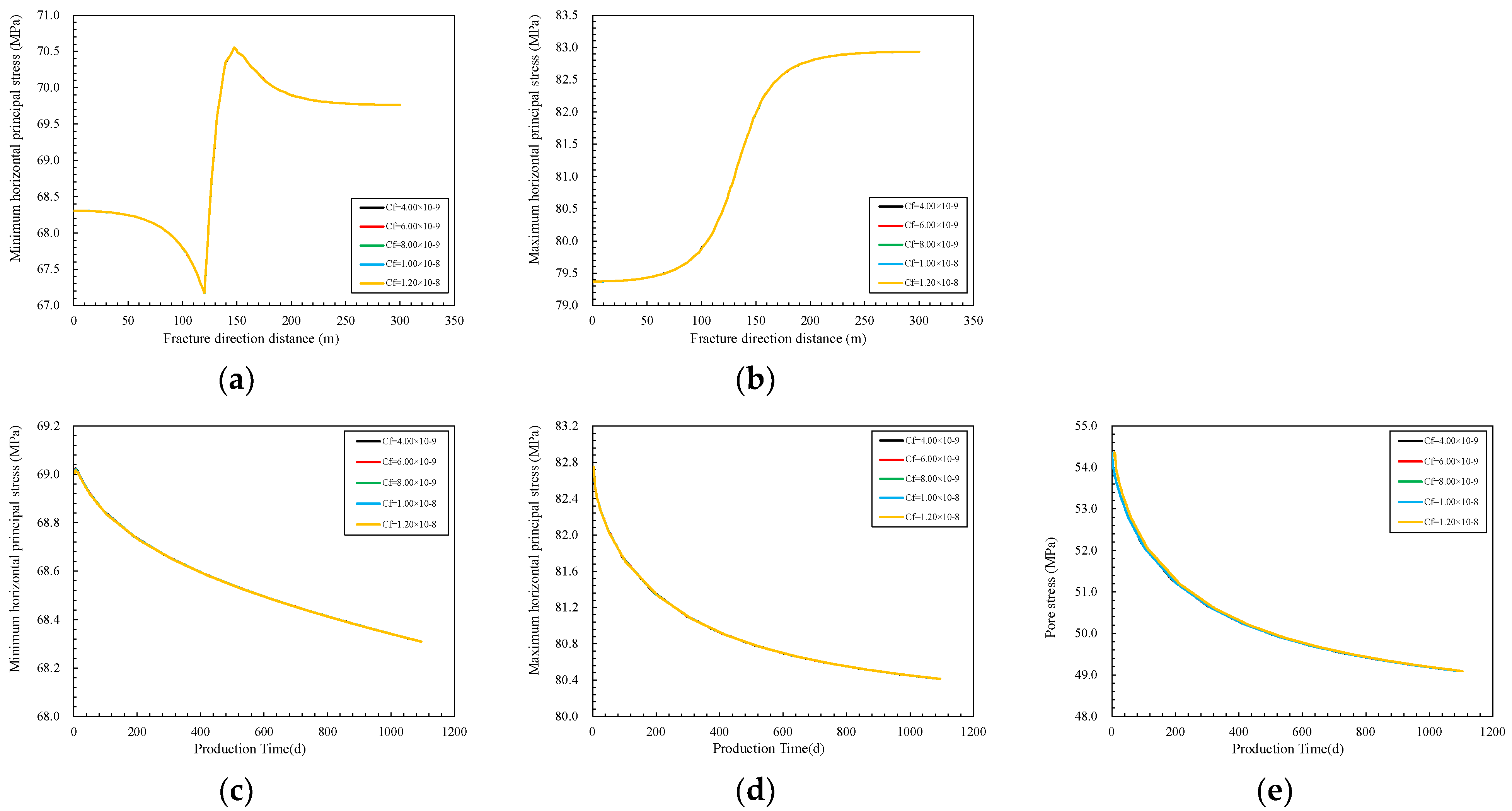
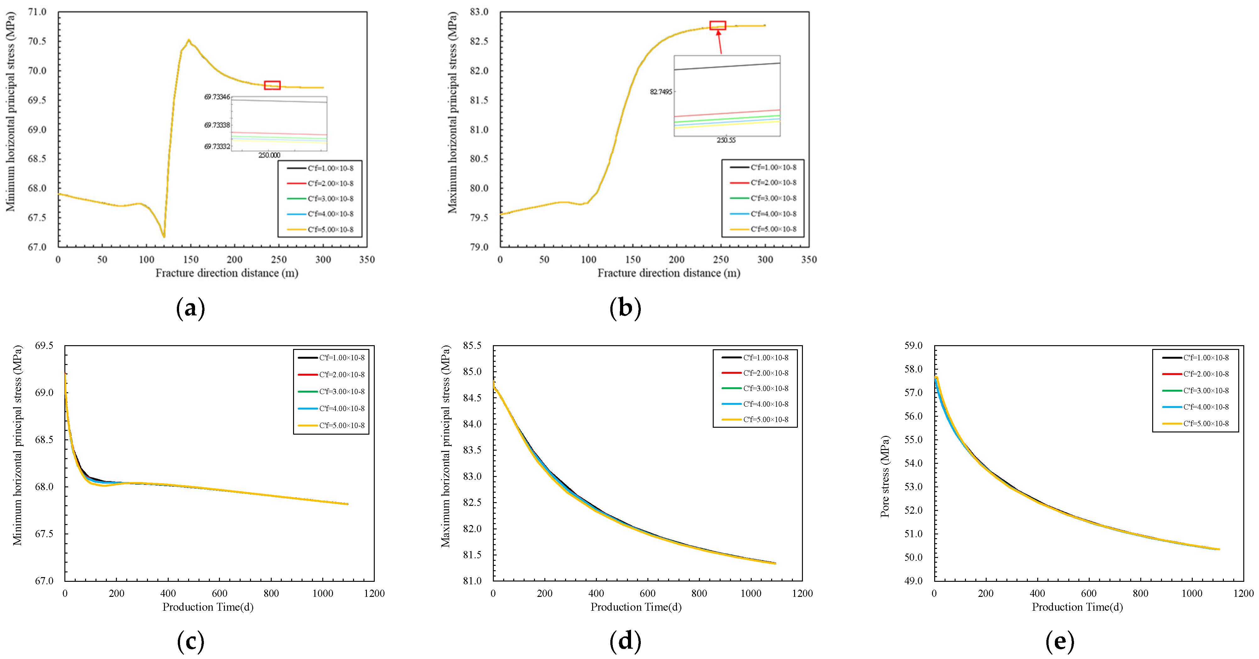
4.3. Compression Coefficient of Main and Secondary Fracture

From Figure 9 and Figure 10, it can be seen that the compression coefficients of the main and secondary fractures have a relatively small impact on the main stress and pore pressure, and the stress curves almost overlap, with changes only within 0.001 MPa. After locally zooming in on the curve, it was found that as the compression coefficient of the main fracture increased, the main stress almost proportionally increased. As the compression coefficient of secondary fractures increases, the main stress decreases, and the larger the compression coefficient of secondary fractures, the smaller the reduction amplitude. As production progresses in reservoirs with different compression coefficients, the difference in stress is also not significant. The reason may be that the presence of cracks causes stress to be localized at and near the crack tip. Even if the compression coefficients of the primary and secondary cracks change, this localization effect may make the change of the overall stress distribution not significant. The compressive coefficient of primary and secondary fractures changes, but the stress does not change much, which may also be the result of the interaction between fractures, healing effect, stress relaxation, nonlinear response of rock, threshold effect of fracture closure, and anisotropy of rock.

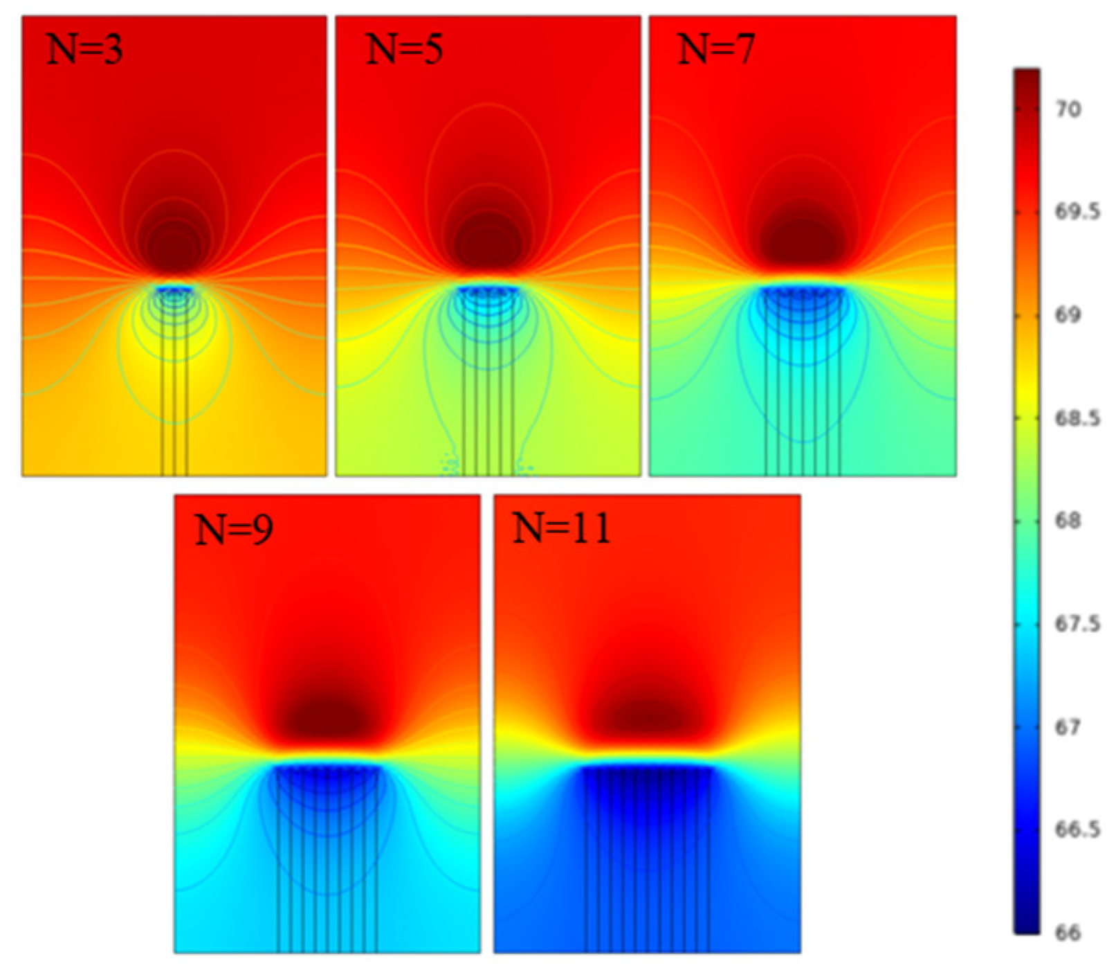
4.4. Number of Main Fracture

From Figure 11a,b, it can be observed that as the number of main fractures increases from 3 to 11, the minimum horizontal principal stress in the fracture area decreases by 1.9 MPa, and the maximum horizontal principal stress increases by 0.64 MPa, with a variation within the range of 2.85%. From Figure 11c–e, it can be seen that as production progresses, the change in the number of fractures has the greatest impact on pore pressure and the smallest impact on minimum principal stress. After the production of 300, the main stress tends to flatten under different fracture numbers, and the pore pressure only tends to flatten after the number of fractures is greater than 9, while the number of fractures is fewer than 9. As production progresses, the pore pressure shows a decreasing trend. From the pressure cloud map 9, it can be observed that after 3 years of production, as the number of main fractures increases, the diffusion range of the low stress area of the minimum horizontal principal stress significantly expands, changing from a semi-circular distribution to a volcanic crater-shaped distribution, and the high stress area at the fracture tip changes from an elliptical distribution to a semi-circular distribution (Figure 12).

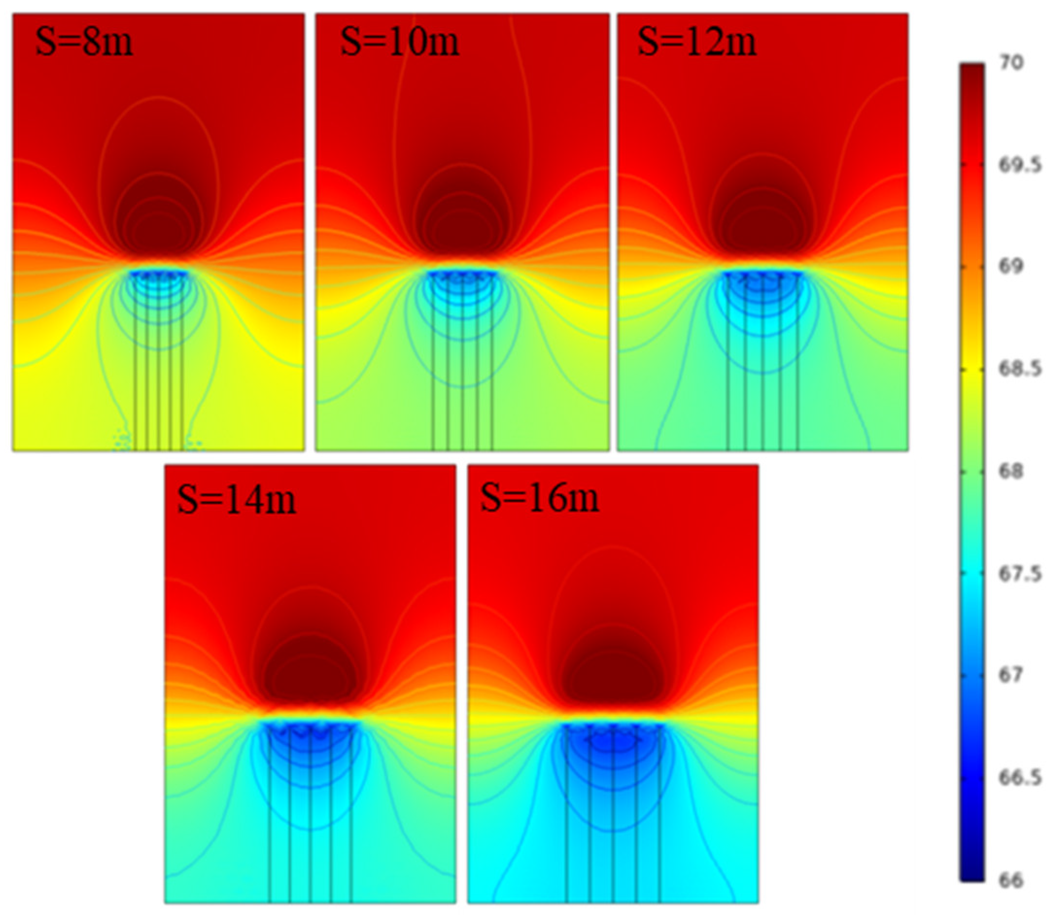
4.5. Main Fracture Spacing

From Figure 13a,b, it can be seen that as the spacing between main fractures increases from 8 m to 16 m, the minimum horizontal principal stress near the wellbore decreases by 0.92MPa, and the maximum horizontal principal stress increases by 0.43 MPa, with a variation range of 1.36%. From Figure 13c–e, it can also be seen that as the spacing between main fractures increases, the decrease in principal stress and pore pressure increases. From pressure cloud map 14, it can be observed that after 3 years of production, as the fracture spacing increases, the low stress zone spreads from the fracture tip to the surrounding areas, and the high stress changes from a circular area to a semi-circular area (Figure 14).

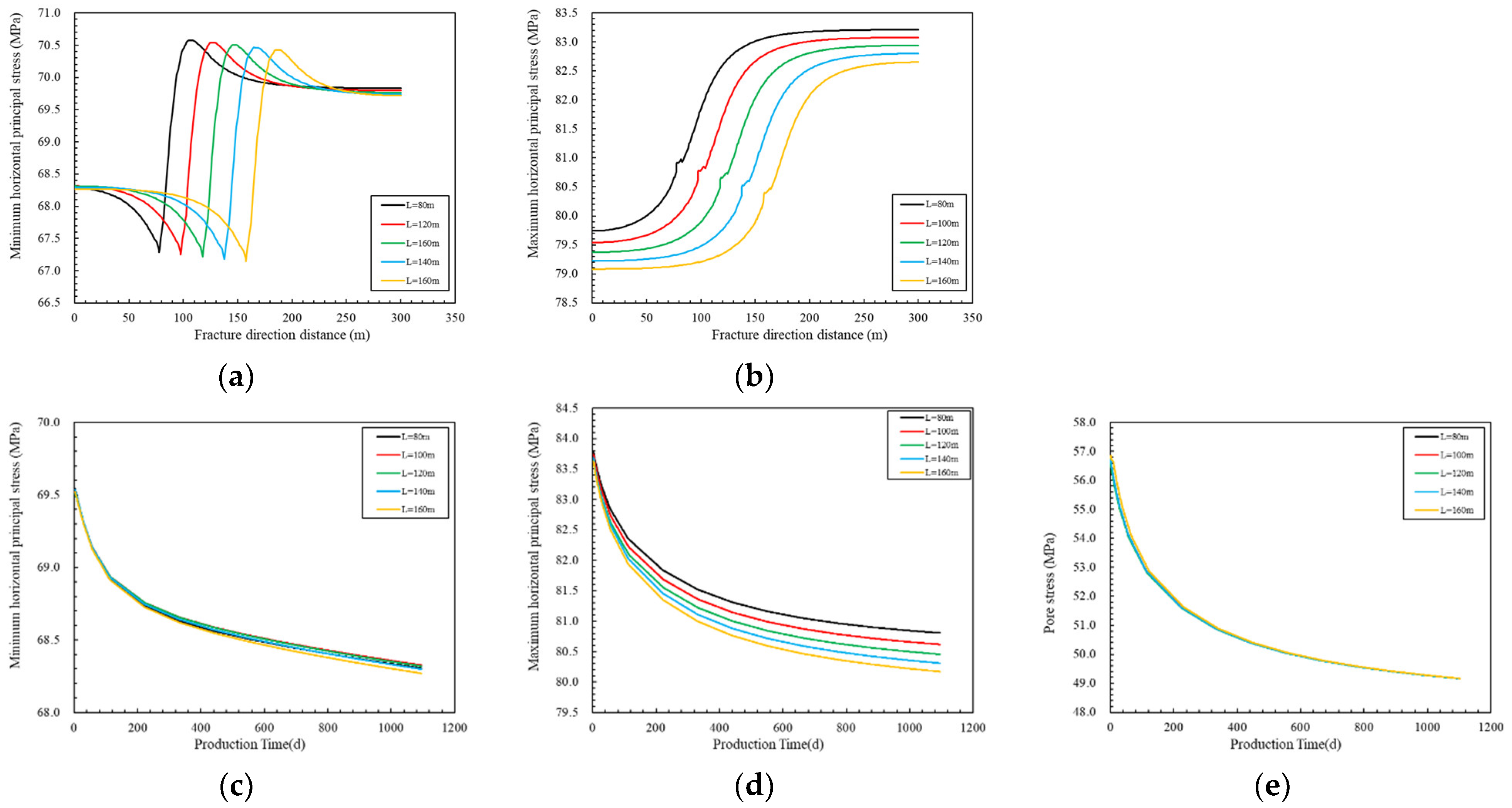
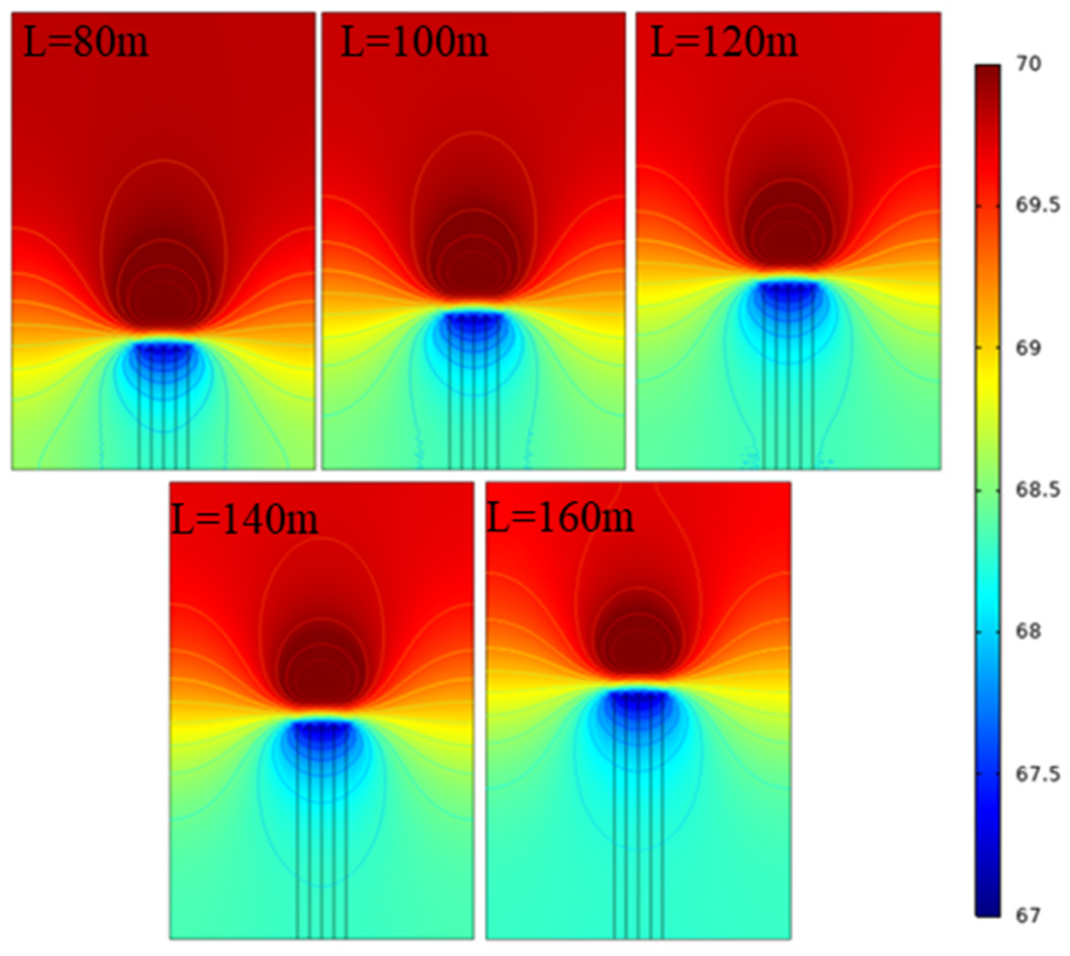
4.6. Main Fracture Length

From Figure 15, it can be observed that as the fracture length increases from 80 m to 160 m, the maximum horizontal principal stress at the fracture opening increases by 0.66 MPa, while the minimum horizontal principal stress decreases by 0.13 MPa. The stress variation is within the range of 0.83%. And as production progresses, the change in the length of the main fracture has a relatively small impact on the principal stress and pore pressure. From Figure 16, it can be observed that as the length of the main fracture increases, the stress distribution shape remains unchanged and the range changes. The minimum horizontal principal stress decreases in the high stress area and increases in the low stress area.

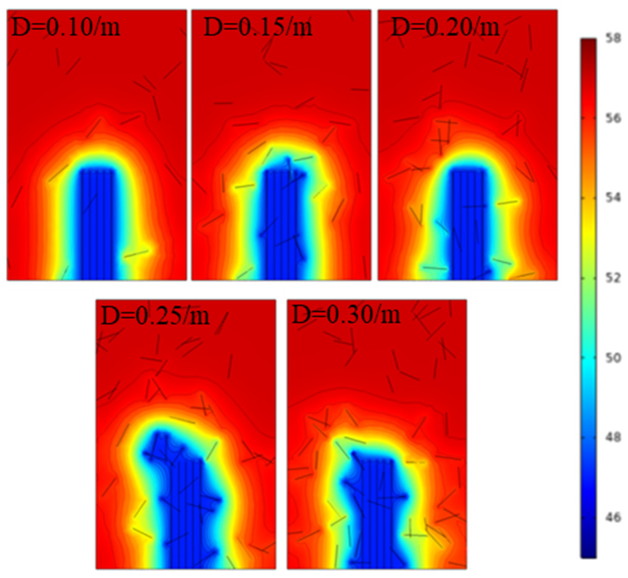
4.7. Natural Fracture Density

In order to investigate the influence of natural fracture density on pressure channeling, the distribution of pore pressure cloud maps under different natural fracture densities was plotted, as shown in Figure 17. From Figure 17 and Figure 18, it can be seen that as the density of natural fractures increases from 0.1 to 0.3, the pore pressure decreases by 1.59 MPa (3.32%), the gradient significantly increases, and the diffusion range of pore pressure significantly expands. In most cases, the higher the density of natural fractures, the larger the reservoir area where the fractures communicate. However, when the density of natural fractures increased from 0.25 to 0.3, the results of the quantitative analysis of the blue area by software show that the difference of the diffusion range between the two is only 0.5%, and there is no obvious change. It can be seen that most natural fractures did not successfully open or their permeability was too low. Therefore, when fracturing multiple clusters of horizontal wells, it is necessary to avoid communicating with natural fracture zones or consider reducing the flow conductivity of natural fractures.

4.8. Natural Fracture Angle

In order to investigate the influence of the natural fracture angle on pressure channeling, the distribution of pore pressure cloud maps under different angles between natural fractures and main fractures was plotted, as shown in Figure 19. From Figure 19 and Figure 20, it can be seen that as the inclination angle increases from 0° to 80°, the pore pressure decreases by 0.39 MPa (0.82%) after 3 years of production. When the angle between the natural fracture and the main fracture is 0°, the artificial fracture can only communicate with the natural fracture on its extension path. As the angle between the natural fracture and the main fracture increases, the artificial fracture is more likely to communicate with the natural fractures on both sides, ultimately leading to the expansion of the pore pressure diffusion area. In the process of horizontal well fracturing, in order to avoid interference between wells, more attention should be paid to the direction of natural fracture development. When fracturing subwells, the appropriate angle with the natural fracture should be selected based on the location of the parent well.

5. Conclusions and Recommendations

Based on the theory of porous media elasticity and the mechanism of fluid solid coupling interaction, a dynamic transformation model for the stress field of fixed pressure production in horizontal wells considering multi-stage stress sensitivity was established. The research conclusion is as follows:

• For low-permeability reservoirs, multi-stage stress sensitivity has a relatively low impact on reservoir stress. As the stress sensitivity coefficients of matrix porosity and matrix permeability increase, the minimum horizontal principal stress value in the entire fracture length direction decreases within the range of 0.27%, the low stress area increases, and the high stress area decreases. With the change of the fracture compression coefficient, the principal stress changes within 0.001 MPa, and the stress distribution pattern does not significantly change.
• The main fracture parameters have a significant impact on the stress field. As the number, spacing, and length of the main fractures change, the main stress varies within the range of 2.85%, 1.36%, and 0.83%, respectively. The number, spacing, and size of the main fractures show a negative correlation, while the length of the main fractures shows a negative correlation.
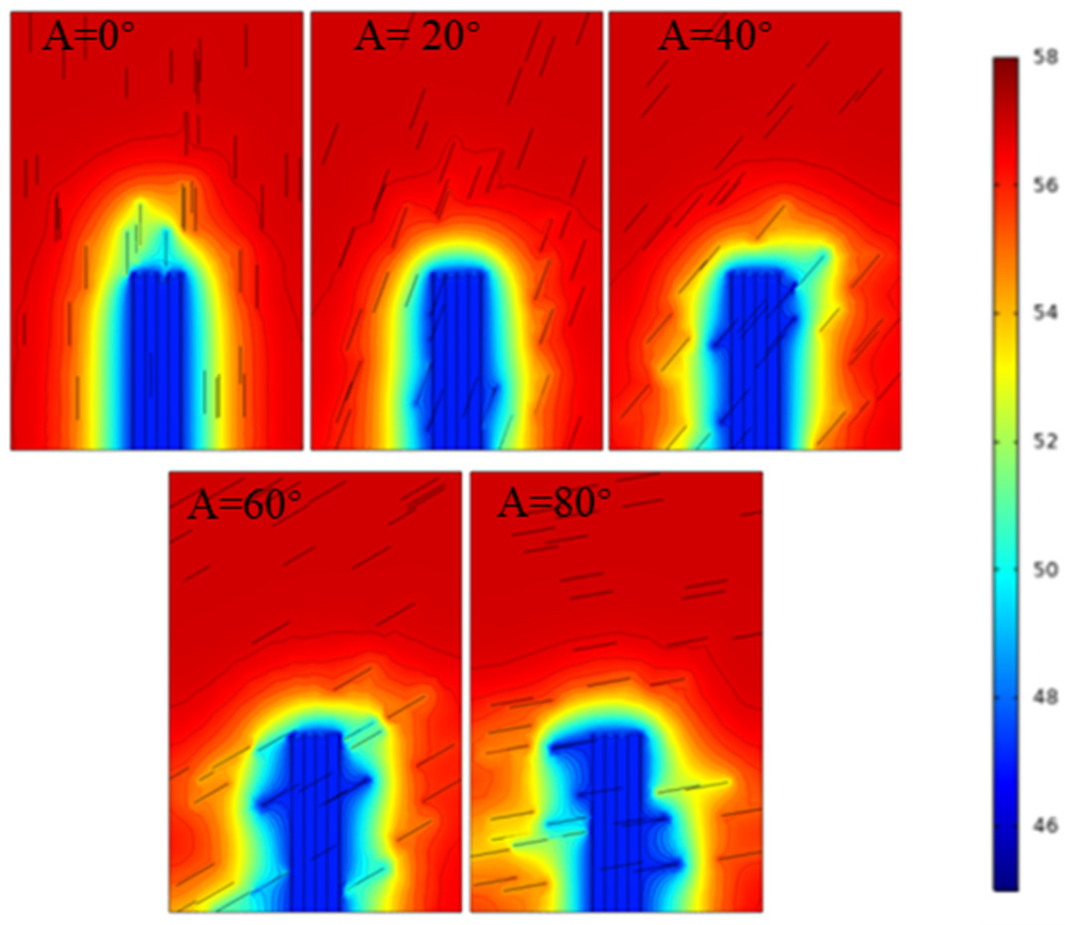
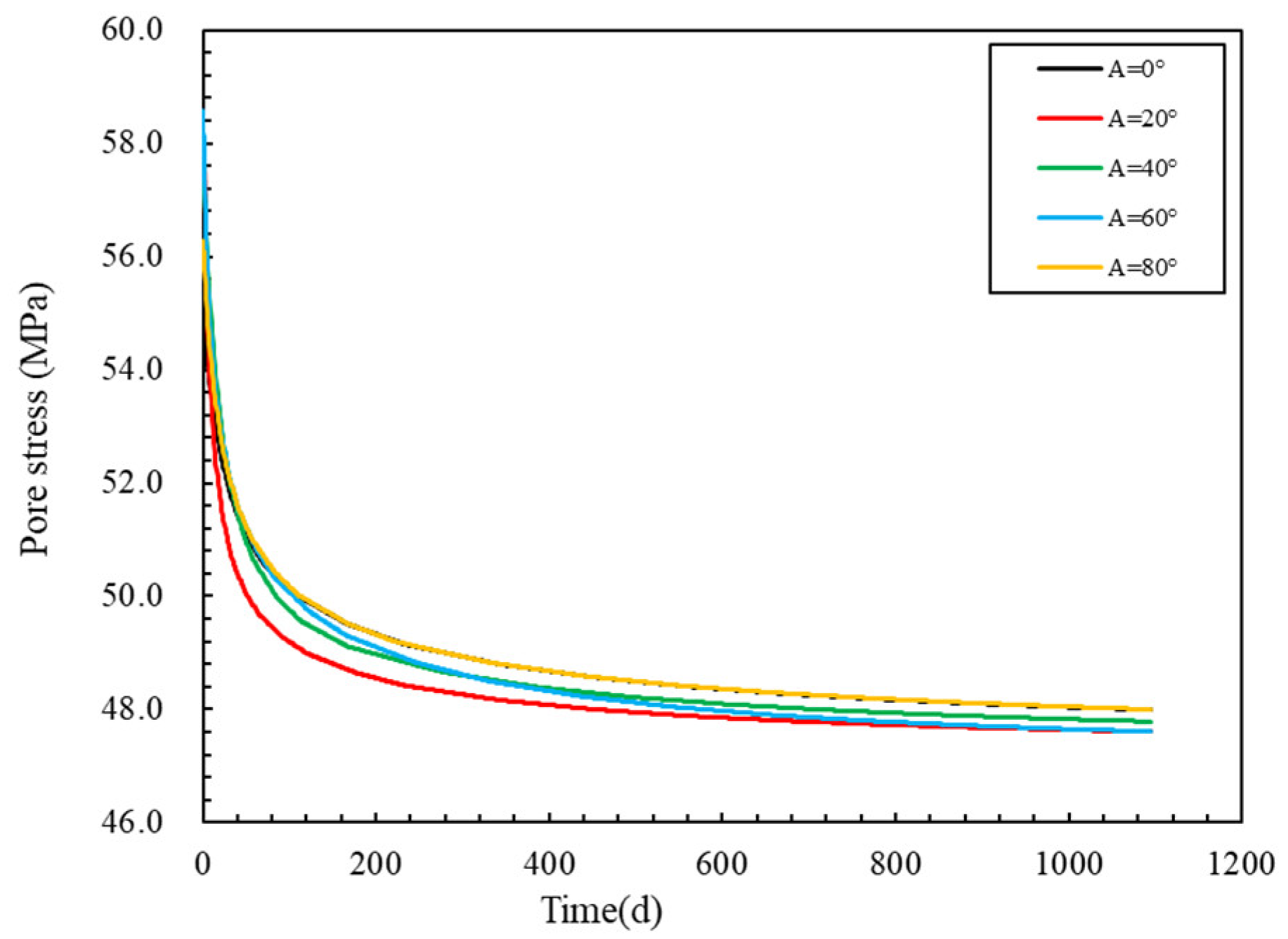
• Random natural fractures have a significant impact on pore pressure, with the density of natural fractures increasing from 0.1 to 0.3, resulting in a decrease of 3.32% in pore pressure and a significant increase in the diffusion area of pore pressure. As the angle between natural fractures increases, it is easier to communicate with the reservoir on both sides of the fracture.
• This type of reservoir should pay more attention to the impact of perforation spacing, perforation cluster number, construction displacement, and natural fracture conditions on the stress field.

References

1. Jia, A.; Wei, Y.; Guo, Z.; Wang, G.; Meng, D.; Huang, S. Development status and prospect of tight sandstone gas in China. Nat. Gas Ind. B 2022, 9, 467–476. [Google Scholar] [CrossRef]
2. Gakhar, K.; Shan, D.; Rodionov, Y.; Malpani, R.; Ejofodomi, E.A.; Xu, J.; Fisher, K.; Fischer, K.; Morales, A.; Pope, T.L. Engineered Approach for Multi-Well Pad Development in Eagle Ford Shale. In Proceedings of the Unconventional Resources Technology Conference, San Antonio, TX, USA, 1–3 August 2016. [Google Scholar]
3. Niu, G.; Sun, J.; Parsegov, S.; Schechter, D. Integration of Core Analysis, Pumping Schedule and Microseismicity to Reduce Uncertainties of Production Performance of Complex Fracture Networks for Multi-Stage Hydraulically Fractured Reservoirs. In Proceedings of the SPE Eastern Regional Meeting, Lexington, KY, USA, 4–6 October 2017. [Google Scholar]
4. Miller, G.; Lindsay, G.; Baihly, J.; Xu, T. Parent Well Refracturing: Economic Safety Nets in an Uneconomic Market. In Proceedings of the SPE Low Perm Symposium, Denver, CO, USA, 5–6 May 2016. [Google Scholar]
5. He, Y.; Guo, J.; Tang, Y.; Xu, J.; Li, Y.; Wang, Y.; Lu, Q.; Patil, S.; Rui, Z.; Sepehrnoori, K. Interwell Fracturing Interference Evaluation of Multi-Well Pads in Shale Gas Reservoirs: A Case Study in WY Basin. In Proceedings of the SPE Annual Technical Conference and Exhibition, Virtual, 26–29 October 2020. [Google Scholar]
6. Liu, H.; Lan, Z.; Zhang, G. Evaluation of Refracure Reorientation in Both Laboratory and Field Scales. In Proceedings of the 2008 SPE International Symposium and Exhibition on Formation Damage Control, Lafayette, LA, USA, 13–15 February 2008. [Google Scholar]
7. Zhang, G.Z.G.; Chen, M.C.M. Dynamic fracture propagation in hydraulic re-fracturing. J. Petrol. Sci. Eng. 2010, 70, 266–272. [Google Scholar] [CrossRef]
8. Mortazavi, A.; Atapour, H. An experimental study of stress changes induced by reservoir depletion under true triaxial stress loading conditions. J. Petrol. Sci. Eng. 2018, 171, 1366–1377. [Google Scholar] [CrossRef]
9. Elliott, I.N.S.A. The opening of a Griffith Crack under internal pressure. Quart. Appl. Math. 1946, 262–267. [Google Scholar]
10. Sneddon, I.N. The Distribution of Stress in the Neighbourhood of a Crack in an Elastic Solid. Proc. R. Soc. A Math. Phys. Eng. Sci. 1946, 229–260. [Google Scholar]
11. Palmer, I.D. Induced Stresses Due to Propped Hydraulic Fracture in Coalbed Methane Wells. In Proceedings of the Low Permeability Reservoirs Symposium, Denver, CO, USA, 26–28 April 1993. [Google Scholar]
12. Zhai, Z.; Sharma, M.M. Estimatina Fracture Reorientation due to Fluid Injection/Production. In Proceedings of the SPE Production and Operations Symposium 2007, Oklahoma City, OK, USA, 31 March–3 April 2007. [Google Scholar]
13. Guan, B.A.S.C.; Li, S.A.; Liu, J.A.; Zhang, L.A.; Chen, S.A. Analysis and optimization of multiple factors influencing fracturing induced stress field. J. Pet. Explor. Prod. Technol. 2020, 10, 171–181. [Google Scholar] [CrossRef]
14. Jia, L.; Peng, S.; Wu, B.; Xu, J.; Yan, F.; Li, Q.; Chen, Y. Research on Quantitative Characterization of 3D Fractures Induced by Hydraulic Fracturing: Insights from Experimental Analysis and Mathematical Models. Rock Mech. Rock Eng. 2023, 57, 1997–2016. [Google Scholar] [CrossRef]
15. Liu, E.; Yao, T.; Qiao, L.; Li, J.; Wang, H.; Gao, Q. Research on the propagation mechanism of hydraulic fractures in infill horizontal wells. Front. Earth Sci. 2022, 10, 1026551. [Google Scholar] [CrossRef]
16. Bajestani, B.M.; Osouli, A. Effect of Hydraulic Fracture and Natural Fractures Interaction in Fracture Propagation. In Proceedings of the 13th ISRM International Congress of Rock Mechanics, Montreal, QC, Canada, 10–13 May 2015. [Google Scholar]
17. Hu, Y.; Gan, Q.; Hurst, A.; Elsworth, D. Hydraulic fracture propagation and interaction with natural fractures by coupled hydro-mechanical modeling. Geomech. Geophys. Geo-Energy Geo-Resour. 2022, 8, 1–26. [Google Scholar] [CrossRef]
18. Shakib, J.T. RETRACTED: Numerical modeling of hydraulic fracture propagation: Accounting for the effect of stresses on the interaction between hydraulic and parallel natural fractures. Egypt. J. Pet. 2015, 231, 557–563. [Google Scholar] [CrossRef]
19. Li, X.L.X.; Wang, J.W.J.; Elsworth, D.E.D. Stress redistribution and fracture propagation during restimulation of gas shale reservoirs. J. Petrol. Sci. Eng. 2017, 154, 150–160. [Google Scholar] [CrossRef]
20. Saberhosseini, S.E.E.S. Optimization of the horizontal-well multiple hydraulic fracturing operation in a low-permeability carbonate reservoir using fully coupled XFEM model. Int. J. Rock Mech. Min. Sci. 2019, 114, 33–45. [Google Scholar] [CrossRef]
21. Mu, S.; Liu, Y.; Lu, Q.; Guo, J.; Yu, H. Numerical simulation of fracture propagation in child wells considering dual-stress field. Eur. J. Environ. Civ. Eng. 2024, 28, 1–17. [Google Scholar] [CrossRef]
22. Mu, S.; Liu, Y.; Wen, Z.; Liu, H.; Guo, J.; Yu, H. Analysis on refracturing of deep fractured sandstone gas well with set production in Tarim Basin. Pet. Sci. Technol. 2023, 42, 1–27. [Google Scholar] [CrossRef]
Figure 1. Schematic diagram of dynamic evolution of stress field.
Processes 12 01652 g001
Figure 2. Geological Model Diagram.
Processes 12 01652 g002
Figure 3. Comparison of formation pore pressure. (a) Validation model. (b) This article’s model.
Processes 12 01652 g003
Figure 4. Comparison of stress in the direction of maximum horizontal principal stress. (a)Validation model. (b)This article’s model.
Processes 12 01652 g004
Figure 5. Comparison of stress in the direction of minimum horizontal principal stress. (a)Validation model. (b)This article’s model.
Processes 12 01652 g005
Figure 6. Changes in the influence of stress sensitivity coefficients of different matrix porosity on horizontal principal stress in A–A′ direction and monitoring point stress. (a) Minimum horizontal principal stress change. (b) Maximum horizontal principal stress change. (c) Monitoring point minimum horizontal principal stress over time curve. (d) Monitoring point maximum horizontal principal stress over time curve. (e) Monitoring point pore pressure over time curve. Where Cp is the stress sensitivity coefficient of matrix porosity.
Processes 12 01652 g006
Figure 7. Cloud map of minimum horizontal principal stress variation under stress sensitivity coefficient conditions of different matrix porosities.
Processes 12 01652 g007
Figure 8. Changes in the influence of stress sensitivity coefficients of different matrix permeability on horizontal principal stress in the A–A′ direction and monitoring point stress. (a) Minimum horizontal principal stress change. (b) Maximum horizontal principal stress change. (c) Monitoring point minimum horizontal principal stress over time curve. (d) Monitoring point maximum horizontal principal stress over time curve. (e) Monitoring point pore pressure over time curve. Where Ca is the matrix permeability stress sensitivity coefficient.
Processes 12 01652 g008
Figure 9. Changes in the influence of different main fracture compression coefficients on the horizontal principal stress in the A–A′ direction and the stress at monitoring points. (a) Minimum horizontal principal stress change. (b) Maximum horizontal principal stress change; (c) Monitoring point minimum horizontal principal stress over time curve. (d) Monitoring point maximum horizontal principal stress over time curve. (e) Monitoring point pore pressure over time curve. Where Cf is the compression coefficient of main fracture.
Processes 12 01652 g009
Figure 10. Changes in the influence of different secondary fracture compression coefficients on the horizontal principal stress in the A–A′ direction and the stress at monitoring points. (a) Minimum horizontal principal stress change. (b)Maximum horizontal principal stress change. (c) Monitoring point minimum horizontal principal stress over time curve. (d) Monitoring point maximum horizontal principal stress over time curve. (e) Monitoring point pore pressure over time curve. Where C’f is the compression coefficient of secondary fracture.
Processes 12 01652 g010
Figure 11. Changes in the influence of different numbers of main fractures on the horizontal principal stress in the A–A′ direction and the stress at monitoring points. (a) Minimum horizontal principal stress change. (b) Maximum horizontal principal stress change. (c) Monitoring point minimum horizontal principal stress over time curve. (d) Monitoring point maximum horizontal principal stress over time curve. (e) Monitoring point pore pressure over time curve. Where N is the number of main fractures.
Processes 12 01652 g011
Figure 12. Cloud map of minimum horizontal principal stress variation under different numbers of main fractures.
Processes 12 01652 g012
Figure 13. The variation curve of the influence of different main fracture spacing on the horizontal principal stress in the A–A′ direction and the stress at the monitoring point. (a) Minimum horizontal principal stress change. (b) Maximum horizontal principal stress change. (c) Monitoring point minimum horizontal principal stress over time curve. (d) Monitoring point maximum horizontal principal stress over time curve. (e) Monitoring point pore pressure over time curve. Where S is the main fracture spacing.
Processes 12 01652 g013
Figure 14. Cloud map of minimum horizontal principal stress variation under different main fracture spacing.
Processes 12 01652 g014
Figure 15. Changes in the influence of different main fracture lengths on the horizontal principal stress in the A–A′ direction and the stress at monitoring points. (a) Minimum horizontal principal stress change. (b) Maximum horizontal principal stress change. (c) Monitoring point minimum horizontal principal stress over time curve. (d) Monitoring point maximum horizontal principal stress over time curve. (e) Monitoring point pore pressure over time curve. Where L is the main fracture length.
Processes 12 01652 g015
Figure 16. Cloud map of minimum horizontal principal stress variation under different main fracture lengths.
Processes 12 01652 g016
Figure 17. Cloud map of pore pressure changes under different natural fracture densities.
Processes 12 01652 g017
Figure 18. Time-varying curves of pore pressure at different natural fracture density monitoring points. Where D is the natural fracture density.
Processes 12 01652 g018
Figure 19. Cloud map of pore pressure changes under different natural fracture angles.
Processes 12 01652 g019
Figure 20. Time-varying curves of pore pressure at monitoring points with different natural fracture angles. Where A is the natural fracture angle.
Processes 12 01652 g020