Abstract
For manufacturing systems such as hot rolling, where there is no wait in the production process, breaks between adjacent production batches provide “opportunities” for predictive maintenance. With the extensive application of industrial robots, a production machine–robot collaboration mode should be considered in system-level predictive maintenance. The hybrid failure mode of machines and dependencies among machines further elevate the difficulty of developing predictive maintenance schedules. Therefore, a novel system-level predictive maintenance method for the no-wait production machine–robot collaborative maintenance problem (NWPMRCMP) is proposed. The machine-level predictive maintenance optimization model under hybrid failure mode, which consists of degradation and sudden failure, is constructed. Based on this, the system-level maintenance optimization model is developed, which takes into account the economic dependency among machines. The maintenance model with the objective of minimizing the total cost is transformed into a Markov decision process (MDP), and a tailored proximal policy optimization algorithm is developed to solve the resulting MDP. Finally, a case study of a manufacturing system consisting of multiple hot-rolling machines and labeling robots is constructed to demonstrate the effectiveness of the proposed method. The results show that the designed algorithm has good performance and stability. Moreover, the developed strategy maximizes the performance of the machine and thus reduces the total maintenance cost.
1. Introduction
Predictive maintenance (PdM) is essential in Industry 4.0, improving production efficiency by predicting and preventing equipment failures [1]. PdM is vital for boosting manufacturing efficiency, prolonging equipment life, and sustaining operations through proactive failure management and reduced downtime [2]. In no-wait production systems, where jobs are processed in sequence without any operational pauses [3]. No-wait production streamlines manufacturing by ensuring a continuous process flow and reducing production times, thus eliminating idle periods [4]. The no-wait production model complicates PdM decision-making, requiring strategic machinery maintenance selection and downtime scheduling.
Intelligent manufacturing progressively integrates advanced technologies into production, showcasing the synergy between smart and intelligent systems [5]. This evolution catalyzes a profound integration of production machinery and robots within Industry 4.0’s collaborative ecosystems, enhancing production efficiency and flexibility [6]. However, this integration introduces complexities to PdM, necessitating an expansion beyond traditional system-level strategies to include the intricacies of robotic systems [7]. Advanced predictive maintenance, powered by analytics and simulations, is crucial for sustaining industrial robots, ensuring uninterrupted operations, and optimizing efficiency with digital twin tech [8].
The research on PdM for multi-machine systems is pivotal, focusing on the Knowledge-Enhanced Reinforcement Learning (KERL) method’s enhanced coordination and optimization in complex environments, which is essential for streamlining maintenance processes as Hu et al. [9] have discussed. Karlsson et al. [10] introduced a robust PdM framework utilizing a hierarchical Gaussian process temporal model (GTM), which was adept at recognizing degradation patterns to ensure more efficient and reliable systems. The value of accurate PdM, grounded in historical manufacturing data, was further explored by Wang et al. [11], who highlighted its importance for informed decision-making. A data-driven hybrid deep learning framework is proposed by Shoorkand et al. [12], integrating PdM with production planning to optimize costs while ensuring demand satisfaction, demonstrating high predictive accuracy and solution quality.
The economic dependency of PdM in multi-machine maintenance is emphasized by Wang et al. [13], influencing cost-efficiency and financial sustainability. Zhou et al. [14] proposed a two-level optimization approach that addresses both system and equipment levels. However, the study identifies a research gap in the economic aspects of predictive maintenance for multi-machine systems, indicating the need for further exploration to exploit the financial benefits of interconnected machinery maintenance fully.
Imperfect maintenance, which does not fully restore system functionality and may perpetuate degradation, poses unique challenges for system-level maintenance. Deep et al. [15] advocated for a multivariate imperfect maintenance model tailored for multi-machine systems, highlighted for its scalability and suitability for large-scale industrial applications through a two-stage estimation method. Mai et al. [16] advanced an optimization model that prioritizes imperfect maintenance to bolster long-term profitability and efficiency within multi-component systems. Zhu et al. [17] constructed a multi-component system maintenance model within a system of systems framework, adept at handling complex failure modes and imperfect prediction signals. Chen et al. [18] introduced an opportunistic maintenance model for multi-machine systems, utilizing a stochastic fuzzy approach and an adaptive immune algorithm to optimize imperfect maintenance and augment production efficiency. Zhang et al. [19] refined multi-state system maintenance by enhancing imperfect strategies to maximize lifecycle benefits.
The maintenance decision-making process becomes intricate in systems that exhibit mixed-failure modes. Jianhui et al. [20] introduced an optimization strategy for multi-indicator systems, applying division models to decipher the intricacies of mixed failure modes and employing a cost-rate approach to guide maintenance decisions. Mullor et al. [21] expanded this strategy to multi-component systems, conducting individualized modeling and selecting the most effective maintenance strategies to balance cost and reliability. Sharifi and Taghipour [22] considered the integration of production and maintenance for a degrading single-machine system, utilizing a probabilistic model and algorithms such as genetic algorithms (GA) to minimize system costs. Zheng and Makis [23] applied a semi-Markov decision process to identify the optimal maintenance actions for systems with dependent failure modes, thereby reducing long-term costs. Qiu et al. [24] developed optimal maintenance policies for systems with competing failure modes, designed with a focus on improving system availability and reducing costs through imperfect repairs and periodic inspections. Liu and Wang [25] delved into the optimal maintenance strategy for warranty products that have multiple failure modes, concentrating on a geometric warranty policy and periodic preventive maintenance, aiming to minimize the life cycle cost rate. The optimal policy is determined through a recursive algorithm. Through this structured and progressive research, the domain of maintenance decision-making under mixed failure modes is thoroughly investigated, contributing significantly to the optimization of maintenance strategies in complex, multi-component systems.
In the realm of Industry 4.0, PdM is recognized as a cornerstone for enhancing operational efficiency and ensuring seamless production flows by preemptively identifying and addressing equipment malfunctions. The intricacies of PdM in no-wait production systems, where continuous process flow is paramount, underscore the necessity for sophisticated, intelligent maintenance strategies that are both proactive and data-driven. This review of the current state of PdM strategies reveals a set of challenges and opportunities that form the basis of our research. The main contributions of this article are as follows:
- (1)
- We present a novel predictive maintenance strategy that specifically addresses economic dependency within a no-wait production system, where machines and robots operate in a collaborative yet financially interlinked environment. This approach provides a more nuanced understanding of maintenance costs and benefits, leading to more informed decision-making.
- (2)
- The study introduces a sophisticated method for modeling equipment failure behavior that encompasses hybrid fault modes. This method enhances the predictive maintenance process by offering a more detailed and realistic representation of potential equipment failures, thereby improving the preemptive actions taken.
- (3)
- By employing a proximal policy optimization (PPO) algorithm, the research navigates the complexities of system-level maintenance optimization in a machine–robot collaborative setting. The PPO algorithm’s application allows for the development of adaptive maintenance policies that respond to the dynamic and interconnected nature of the production environment.
- (4)
- The findings establish a new benchmark for predictive maintenance in industrial applications, particularly in steel production, where the integration of economic factors and predictive analytics results in a strategy that is both scientifically sound and operationally efficient, setting a precedent for future research and industry practices.
The remainder of this paper unfolds as follows. Section 2 formulates the predictive Maintenance strategy for the no-wait production machine-robot collaborative maintenance problem (NWPMRCMP). Section 3 develops the system-level collaborative predictive maintenance optimization model. Section 4 describes the designed decision algorithm based on deep reinforcement learning (DRL). Section 5 verifies and analyzes the model through a comprehensive case study. Section 6 concludes the paper with key findings.
2. Predictive Maintenance Strategy Formulation for NWPMRCMP
2.1. Problem Statement
In the steel industry, the production machinery and robots on the hot rolling production line play a crucial role as automated equipment. The hot rolling production line machinery is responsible for the core processes such as heating, rolling, and cooling of steel materials, while the robots are tasked with the precise printing and attachment of product identification, exerting a significant influence on product traceability and brand reputation. These devices must operate continuously and stably under harsh conditions, like high temperatures and humidity, and meet the “no-wait” requirement of production continuity, which aims to minimize downtime to ensure production efficiency. Therefore, ensuring the stable operation of these devices, reducing the incidence of faults, and improving maintenance efficiency is decisive for the overall efficiency and cost control in steel production, becoming a significant issue faced by steel enterprises.
In the context of “no-wait” production characteristics, the issue of synergistic maintenance between production machinery and robots is exceptionally prominent. The continuous nature of production demands that any equipment failure be met with a swift and efficacious response to prevent the stagnation of the production process and to mitigate significant economic losses. Thus, the central question of this research is how to ensure the continuity of production while achieving effective collaborative maintenance between production machinery and robots. This involves not only the physical linkage and functional alignment of the equipment but also a deep optimization of the inter-machine collaborative maintenance strategies.
Moreover, the hybrid failure modes of equipment and economic dependency among equipment (including production and robot) add further intricacy to this investigation. The term “hybrid failure mode” denotes that equipment may experience both sudden and gradual degradation failures simultaneously. Sudden failures are characterized by abrupt onset and unpredictability, leading to production stoppages. On the other hand, gradual degradation failures manifest as a progressive decline in equipment performance, resulting in increasing costs over time that correlate with the cumulative failure rate of the equipment. This economic dependency emphasizes that collectively maintaining multiple devices may result in lower costs compared to individual maintenance efforts combined. Take the hot-rolling manufacturing systems, for example—the economic dependency is mainly reflected in the downtime loss. Since the production process cannot be stopped, maintenance can cause the entire system to shut down [18]. Therefore, downtime loss is considered in the cost of maintenance actions. When multiple pieces of equipment are maintained simultaneously, the downtime depends on the maximum value of the time required for each maintenance action. As a result, the downtime loss is reduced compared to maintaining each equipment individually. Therefore, optimizing maintenance strategies under hybrid failure modes and reducing overall maintenance expenses through an analysis of economic dependency is another crucial aspect addressed by this research.
2.2. Overall Framework of the Proposed Method
In a no-wait production environment, the construction of a predictive maintenance model for individual equipment begins with an in-depth understanding of equipment failure behavior. This study employs a Weibull-distribution-based approach to characterize the failure probability of motors and fans, determining the shape and scale parameters through historical maintenance data analysis and simulated failure experiments. These parameters provide a mathematical foundation for assessing equipment health and predicting potential failures. Subsequently, by defining maintenance decision variables, including the timing and type of maintenance operations, an optimization model is established to minimize maintenance costs and production losses due to failures. The model dynamically adjusts maintenance strategies through continuous equipment state monitoring, aiming for cost–benefit maximization.
For production machinery and robots, the construction of a system-level maintenance optimization model considers the interdependencies and constraints among equipment to achieve collaborative optimization. This model expands upon the single equipment model by incorporating additional dimensions for equipment sequence and updating decision variables for multiple devices within the production system. By analyzing structural, resource, and economic interdependencies among equipment, this study formulates an integrated maintenance strategy that optimizes maintenance plans under limited resources, considering dependencies and collaborative relationships. Moreover, the model accounts for the impact of maintenance operations on equipment status, such as the adjustments to service life and cumulative failure rate due to perfect and imperfect maintenance, thus accurately reflecting the contribution of maintenance activities to system reliability.
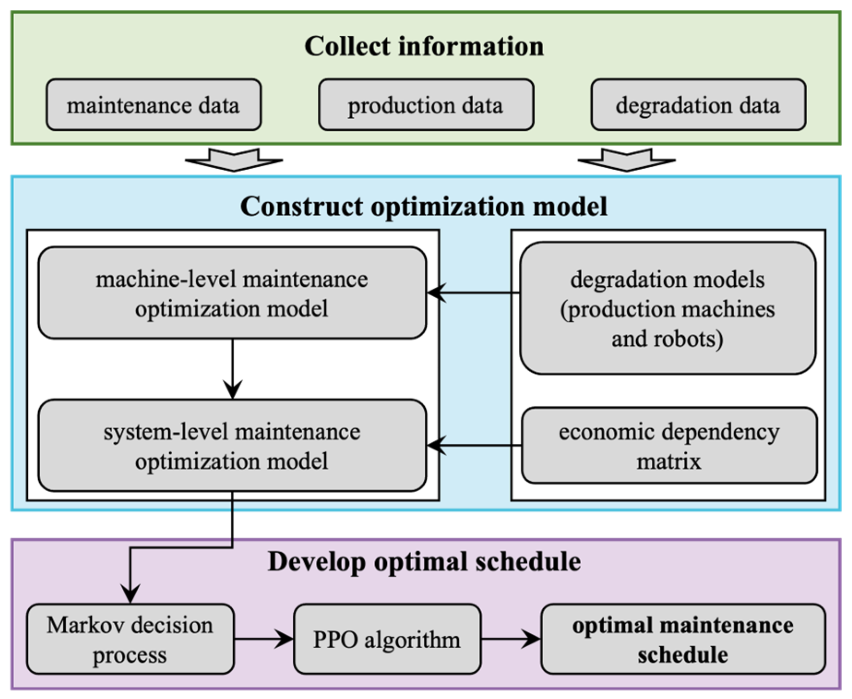
Given that the system optimization model can be transformed into a Markov decision process (MDP) and that the optimization problem is characterized by an infinite horizon MDP with a continuous state space, this study employs a PPO-algorithm-based intelligent decision-making approach. As a policy gradient method, PPO directly learns the optimal policy by parameterizing and optimizing the policy function, effectively handling large-scale state and action spaces. In this research, the PPO algorithm is utilized to solve the system-level maintenance optimization problem. Through interactions with the environment, the agent continually updates its policy to maximize long-term cumulative rewards. Utilizing this method, this study successfully develops an intelligent maintenance decision support system that provides scientific and efficient decision-making for the predictive maintenance of steel production equipment. The specific framework of the article is shown in Figure 1 below.
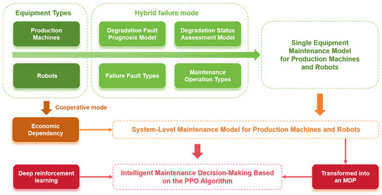
Figure 1.
The research framework of the proposed method.
3. System-Level Collaborative Predictive Maintenance Optimization Model
Based on the developed system-level maintenance strategy, the process of developing optimization model and formulating the optimal maintenance schedule for no-wait production machine-robot collaborative maintenance problem is shown in Figure 2. Each step is briefly described below.
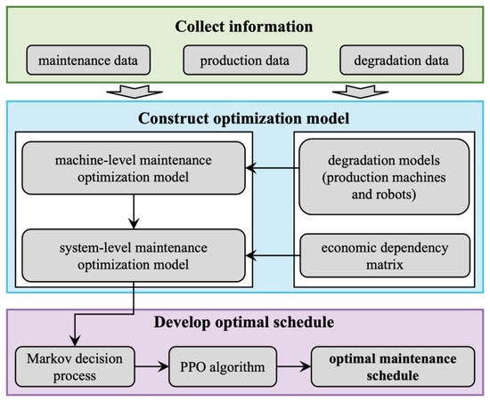
Figure 2.
Flowchart of the decision-making process for NWPMRCMP.
Step 1. Collect information. The purpose of this step is to provide a basis for developing maintenance optimization model. The information collected includes maintenance data, degradation data, and production data.
Step 2. Construct optimization model. The degradation models of production machines and robots are constructed using the collected data. Furthermore, machine-level maintenance optimization model is constructed. The economic dependency matrix is built by analyzing the production and maintenance data. On this basis, a system-level maintenance optimization model is obtained.
Step 3. Develop optimal schedule. The constructed system-level maintenance optimization model is transformed into a Markov decision process, and a PPO algorithm is developed to formulate the optimal maintenance schedule. The details of the PPO algorithm are introduced in Section 4.
3.1. Machine-Level Maintenance Model under Hybrid Fault Mode
In this section, we explore the complexities of a machine-level maintenance model that addresses the hybrid fault modes encountered by production machinery and robots, integral components of the hot-rolling production line. These critical assets are susceptible to a variety of failure causes, such as gear abrasion in production machinery and actuator malfunctions in robots, as well as software aging that affects both types of equipment. The model must contend with both sudden failures, which necessitate immediate intervention, and degradation faults, which unfold over time and require vigilant monitoring and predictive maintenance strategies. Based on the monitoring results of the equipment’s current state at each checkpoint, the most appropriate maintenance operation is selected. Maintenance is not conducted when the equipment is in a satisfactory condition. Conversely, maintenance actions are taken when the probability of sudden failures is excessively high or when there is a significant accumulation of degradation-type failures. In this context, imperfect maintenance is denoted by , while perfect maintenance corresponds to . The maintenance strategy is generally shown in Figure 3.

Figure 3.
Maintenance strategy for a single equipment operation process.
The Weibull distribution is chosen to describe the failure behavior of production machinery and robots due to its ability to model both sudden and gradual degradation failures, reflecting the varying rates of failure occurrence over time and the different failure modes observed in historical maintenance data [26,27]. We employ the Weibull distribution to characterize the failure behavior of machinery, leveraging its versatility to model both sudden and degradation failures through shape and scale parameters. The specific expressions are shown in Equation (1):
where is the random variable representing the service duration of the equipment. The scale parameter is denoted by , and the shape parameter is represented by . Based on the above model, reliability, cumulative failure probability and risk rate can be easily obtained. The parameters of the Weibull distribution are estimated through an extensive analysis of historical maintenance data, enabling a probabilistic framework for the prediction of future failure instances in both production machinery and robots. With this framework, we can seamlessly integrate various maintenance strategies that cater to the distinct needs of machinery and robots at different stages of their operational lifecycles.
Incorporating the dimensions of maintenance time and type, the decision variables are defined as binary variables, denoted as , representing whether the th type of maintenance is performed within the th interval. The values of correspond to no maintenance, imperfect maintenance, and perfect maintenance, respectively. represents the sequence numbers of the intervals.
Perfect maintenance resets equipment condition to its original state, implemented by nullifying the service duration and cumulative failure rate. Imperfect maintenance partially restores equipment performance, introducing an attenuation factor to the service duration and accumulated failure rate. Emergency repairs are undertaken post-sudden failures to restore equipment functionality, encapsulated within the sudden failure cost category, without affecting the equipment’s existing state evolution. With no maintenance, the equipment’s service time and cumulative failure rate adhere to the Weibull distribution. To facilitate expression, the state update equation can be formally unified as shown in Equations (2) and (3):
where the state update equations for the three maintenance operations exhibit a shared characteristic, with an attenuation factor introduced for each operation—denoted by for no maintenance, imperfect maintenance, and perfect maintenance, respectively—with values of . Additionally, it is noted that at a given inspection point, only one maintenance operation can be selected.
The predictive maintenance model at the machine level is constructed with decision variables that encapsulate the timing and type of maintenance actions. The objective function is designed to minimize the sum of maintenance costs and downtime losses, subject to constraints that reflect the operational and health status of the equipment. A critical aspect of this model is the dynamic updating of maintenance strategies based on real-time monitoring of equipment performance and accumulated failure rates. The objective function and constraint equations of the model are summarized as shown in Equations (4)–(8):
where the cost of degradation-type failures is denoted by . For sudden failures, the probability of occurrence is and the cost per incident is . Each maintenance decision directly incurs corresponding maintenance costs, including additional expenditures such as production line downtime and operational fees. These costs are denoted by ; corresponds to no maintenance, imperfect maintenance, and perfect maintenance, respectively.
3.2. System-Level Maintenance Optimization Model Considering Economic Dependency
In constructing a system-level predictive maintenance model, it is imperative to extend beyond the scope of individual equipment predictive maintenance models and consider the interplay among multiple devices within a production line. Beyond the mere increase in the number of devices under scrutiny, a critical factor that necessitates attention is the interdependence that exists between the devices, which precludes independent decision-making for each device. This chapter takes into account two types of relationships, including structural interdependencies and resource interdependencies, to establish a system-level predictive maintenance model for an actual hot rolling production line.
In terms of structural dependency, the production line system studied in this paper is a hybrid system composed of multiple production machines and robots arranged in a series-parallel configuration. For ease of exposition, the system-level model incorporates an additional dimension, denoted by , which represents the sequence numbers of the devices within the system. The system’s reliability , cumulative failure , and failure rate can also be readily derived through the series-parallel combinatorial relationships.
Subsequently, the resource interdependencies within the production line are considered. Resource interdependency refers to the maintenance of multiple devices being contingent upon the same shared resource, such as a finite number of maintenance tools, spare parts, or personnel.
Lastly, the economic interdependencies within the production line are considered. This pertains to the situation where the collective cost of joint maintenance for multiple devices is less than the aggregate cost of independent maintenance for each device. The economic interdependencies of the equipment will be reflected in the cost calculations. For ease of expression, new variables and a matrix of order are introduced as shown in Equations (9) and (10):
where is introduced to represent whether the th device undergoes maintenance during the th interval.
Consequently, the objective function and constraint equations of the system-level predictive maintenance model are summarized as shown in Equations (11)–(15):
In contrast to the predictive maintenance decision model for individual equipment, the total cost representation in the system-level model now incorporates the calculation of cost savings due to economic interdependencies between devices. The constraints have been augmented with the computational method for the new variable , and the subscripts for the remaining variables in the constraints have been updated.
4. Optimization Algorithm Based on DRL
Furthermore, the system-level model is transformed into an MDP to harness the power of DRL algorithms for solution optimization. The overall Markov decision process is shown in Figure 4.

Figure 4.
Schematic diagram of Markov decision process.
This transformation involves defining the state space, action space, transition probabilities, and reward functions within the MDP framework, ensuring that the model adheres to the Markov property for effective decision-making. The process of demonstrating that the predictive maintenance model constructed in Section 3 uses, adhering to the Markov property, is as follows:
It is known that , satisfies different state transition equations based on the values taken by the random variable . Moreover, these transitions exhibit the property of being memoryless. The process of proof is as shown in Equations (16)–(23):
① :
② :
③ :
It was discovered that:
In the final analysis, it was determined that the transition to the next state is solely dependent on the current state and the action taken at the present moment. The reward obtained at the current moment is also exclusively contingent upon the state and action at that instant. Both exhibit the property of being memoryless, fulfilling the fundamental assumptions of a MDP. This framework allows for subsequent optimization through DRL.
Reinforcement learning tasks are typically characterized using the framework of the Markov decision processes (MDPs). The specific interaction process is as follows:
State Space : , given the total duration , is divided into intervals, and the set of all possible states at each inspection point includes all relevant features used to guide maintenance decisions. Specifically, it can be represented as , which includes the service duration and cumulative failure rate of the equipment. The distribution of states over time is discrete, while the specific feature values have a continuous range, being uncountable and non-enumerable.
Action Space : , given the total duration , is divided into intervals, representing the collection of all possible maintenance actions at each inspection point. The distribution of actions over time is discrete, and the specific values of actions are also finite and discrete.
State Transition Function : Describes the probability of transitioning to another state after taking a certain maintenance action in a certain state.
Reward Function : describes the reward obtained after performing a certain action in a certain state. Since the goal in reinforcement learning is often to maximize the total reward, the reward is defined as the opposite of the failure cost [as shown in Equation (24)].
In reinforcement learning, the objective of the agent is to maximize the total reward obtained—that is, to maximize the long-term cumulative return. Consequently, the concept of the subsequent expected return is introduced, and the optimization target of the problem is to maximize , as shown in Equaton (25):
where the discount factor, denoted by , , plays a pivotal role in determining the trade-off between the value of immediate rewards and those that are anticipated in the future. In the present study, the significance of rewards at various time points is considered to be equal. Thus, .
Following the definition of the expected future return , it is possible to further assess the desirability of the agent being in a given state and the efficacy of performing a given action within that state. Integrating the explanation of the agent’s policy , the value function for state . Under the specific policy can be defined, denoted as , as shown in Equation (26):
where represents the expectation of a random variable under a policy , and . denotes the domain space of states having the same dimensionality as the states themselves. Subsequently, this function is referred to as the state-value function of the policy, denoted as .
Similarly, we can define the action–value function for a policy, denoted as shown in Equation (27):
Both of the aforementioned value functions can be formulated using recursive relations, specifically in the following forms (see Equations (28) and (29)):
Equations are referred to as the Bellman equations for and , respectively. These equations express the relationship between the value function of a state (or a state–action pair) and the value functions of its subsequent states (or state–action pairs).
The PPO algorithm, the full name of which is proximal policy optimization, is a policy gradient method. The PPO algorithm makes several modifications based on the aforementioned policy gradient methods, including updating the gradient estimate, using the GAE method to estimate the advantage function, importance sampling, and proximal policy optimization clipping. The specific steps of the PPO algorithm are based on improvements to policy gradients and the detailed implementation approach is outlined in Algorithm 1 as follows:
| Algorithm 1. Pseudocode of the PPO Algorithm |
| Input Parameters: State Space , Reward Space , Action Space , Learning rate, Number of network update steps , etc. |
| Initialization: policy network , value network , Advantage function estimation parameters, optimization parameters. |
| For each training epoch |
| Randomly initialize the state , create a new dataset |
| For each time step |
| Perform the current action given by the policy network |
| Execute the action , obtain the current reward and the next system state |
| Store the sample in the dataset |
| End |
| For each sample |
| Calculate the predicted value of the next state: |
| Calculate the target value: |
| Calculate the temporal difference error: |
| End |
| Calculate the advantage function in reverse order: |
| Calculate the ratio of the new to old policy: |
| Calculate the policy network loss function: |
| Calculate the value network loss function: |
| Back propagate to update the parameters of the policy network and the value network . |
| Update the parameters of the old policy network: . |
| End |
| Output Results: |
Next, the key parts of Algorithm 1, including the GAE approach to estimating the dominance function, importance sampling, and approximate policy optimization clipping, are described in detail.
In this problem, the rewards are all negative and a baseline is introduced to make the rewards both positive and negative. Additionally, a discount factor is incorporated to correctly estimate the expected reward at a given moment. Based on these considerations, the concept of the advantage function is introduced, denoted as . The advantage function refers to the expected reward for taking a certain action in a certain state compared to the value function of that state (see Equation (30)).
The gradient estimation using the advantage function is shown in Equation (31):
In actual training, the PPO algorithm employs the GAE (generalized advantage estimation) method to estimate the advantage function as shown in Equation (32):
where , is the smoothing factor, and is the discount factor. This formula effectively performs a weighted average of the temporal difference errors with weights that exponentially decay as the step size increases. The use of the GAE method efficiently reduces the variance in gradient estimation, thereby lowering the number of samples required for training.
The PPO algorithm indirectly expands the amount of training data through importance sampling, which saves computational costs and enhances training efficiency. The mathematical expression of importance sampling is shown in Equations (33) and (34):
Furthermore, the likelihood objective function to be optimized can be derived, as shown in Equation (35):
Additionally, the PPO algorithm aims to ensure that the difference between the new and old policies is within a certain range during each policy update step. To achieve this, the clipping function . is designed to limit the ratio of the new to old policy within a specific interval, . The update of the likelihood objective function is shown in (36):
The PPO algorithm does not utilize an experience replay mechanism; it only uses experiences generated by the current policy to update the network rather than experiences generated by historical policies. This ensures a high degree of consistency between the policy and the value function, meaning that the value function can always accurately estimate the performance of the current policy. After each episode of interaction with the environment to sample continuous data, the algorithm uses stochastic gradient ascent to optimize a likelihood objective function, thereby improving the policy. Its characteristic is that it allows for multiple small-batch updates rather than performing a single gradient update per data sample as in standard policy gradient methods.
5. Case Study
5.1. Optimal Maintenance Policy
In this paper, the 1580 hot rolling manufacturing system is used as a research object to demonstrate the sophistication of the developed method. This study has been authorized by Shanghai Baosight Software Co. Ltd. (Shanghai, China) for reasonable use of scenarios, data, and field knowledge. As a typical no-wait production process, the slab from the heating furnace is transferred to the roughing mill for rolling after dephosphorization. After two rounds of roughing, the WIP is sent to the finishing mill after heat preservation in the side heating furnace. The strip from the finishing mill is coiled into the final product, which is labeled by robots and stored in the warehouse. In this case study, a manufacturing system consisting of heating furnace (Machine 1), descaling box (Machine 2), two roughing mills (Machines 3 and 4), side heating furnace (Machine 5), finishing mill (Machine 6), coiler (Machine 7), and two labeling robots (Machines 8 and 9) is studied. The schematic diagram of the studied hot rolling manufacturing system is shown in Figure 5.

Figure 5.
Schematic diagram of the studied hot rolling manufacturing system.
Next, the application of the proposed method is presented. Considering the enterprise’s business competition and confidentiality needs, partial processing is performed according to the actual data to generate simulation data, but this does not affect the method’s validation and comparison. The data collected include degradation data, maintenance data, and production data. The raw degradation data contain multidimensional features of the sensor signals. Based on methods such as metric learning [28], these features are fused into one-dimensional health indicators. Combined with the maintenance data, the parameters of the degradation model, namely Weibull distribution, are estimated by the maximum likelihood estimation method. The degradation of each production machine obeys a Weibull distribution with a scale parameter of 15 and a shape parameter of 0.33. The degradation of the two labeling robots is modeled as a Weibull distribution with a scale parameter of 80 and a shape parameter of 15. The length of the operation horizon is 1000 days, and the time interval between each maintenance opportunity is 1 day. In addition, based on production data and maintenance data, the degradation failure cost and the sudden failure cost are = 10 (unit: USD 100) and = 50 (unit: USD 100), respectively. The imperfect maintenance cost and the perfect maintenance cost are the same for each machine. The imperfect maintenance cost is 12 (unit: USD 100), and the perfect maintenance cost is 20 (unit: USD 100). The attenuation factor for imperfect maintenance is 0.25. The economic dependency matrix among machines is as follows:
Since the resulting NWPMRCM problem is converted into an MDP, the tailored PPO algorithm is applied to determine the optimal maintenance schedule. The designed PPO algorithm is written based on PyTorch, in which the maximum number of iterations is 1000. In addition to the input and output layers, both the policy network and the value network have a hidden layer that contains 16 neurons. The Adam optimizer and rectified linear unit (ReLu) activation function are chosen for the agent training. The initial learning rate is set to 0.001 and 0.01 for the policy network and the value network, respectively. The smoothing factor of the advantage function is 0.95. The truncation parameter of the clip function is 0.2. The parameters of PPO algorithm are tabulated in Table 1.

Table 1.
Parameters of PPO algorithm.
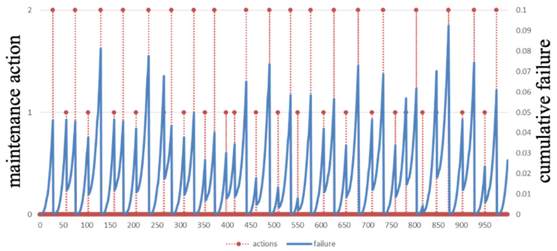
With the prepared-degradation- and maintenance-related information and the designed PPO algorithm, the optimal predictive maintenance schedule’s total maintenance cost is 900.8815. For example, the maintenance schedule for Machine 3 is shown in Figure 6. The type of maintenance action is denoted by the red line, and the change in cumulative failure of the machine during operation is marked by the blue line.
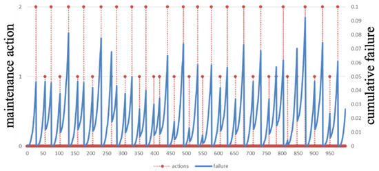
Figure 6.
The optimal maintenance schedule for Machine 3.
The results in Figure 6 show that imperfect maintenance will be performed first to enable regular operation when the cumulative failure reaches a certain level. Then, perfect maintenance will be performed to restore the system to its optimal state and to diminish the hidden problems left by imperfect maintenance. In addition, it can be noticed from Figure 6 that the periodicity of maintenance and the choice of maintenance action are not regular. This phenomenon is due to the fact that the economic dependency of the equipment is taken into account at the same time when developing the maintenance schedule. The off-cycle maintenance schedule further proves that the developed maintenance strategy is flexible.
5.2. Discussion
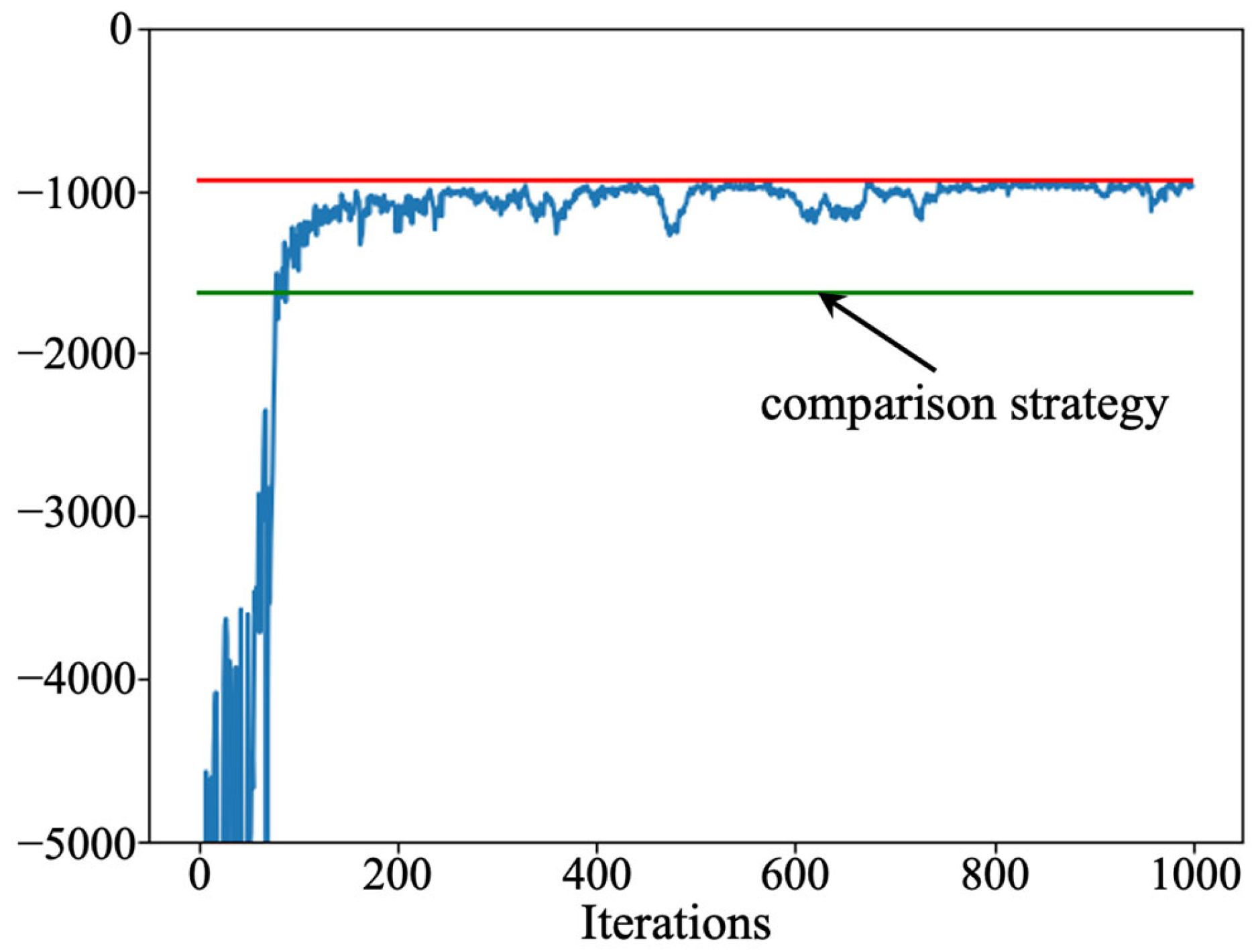
Firstly, to verify the effectiveness of the developed strategy, we compare it to the control-limit-based maintenance strategy [29]. In the comparison strategy, whether a maintenance action is executed or not depends on the failure risk. When the failure risk exceeds the control limit, appropriate maintenance actions—including do nothing, imperfect maintenance, and perfect maintenance—are selected. To facilitate the comparison, the relevant parameters in both methods are the same. The cumulative failure control limit of the comparison strategy is 0.2. Moreover, the optimization objective of the comparison strategy is also to minimize the total cost. The maintenance costs of the two strategies are illustrated in Figure 7.
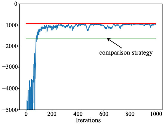
Figure 7.
Results comparison under proposed strategy and control limit strategy.
In Figure 7, the blue line indicates the training process of the designed PPO algorithm, the red line indicates the minimum maintenance cost of the developed strategy, and the green line indicates the maintenance cost of the compared strategy. The results show that the designed PPO algorithm stabilizes after 300 rounds of iterations, and the obtained maintenance cost is better than the compared strategy. This phenomenon implies that the developed strategy is able to improve the machine performance utilization to a greater extent. Meanwhile, from Figure 7, it can be found that the maintenance cost of the developed maintenance strategy is less than that of the comparison strategy. This phenomenon is because the developed strategy does not have fixed control limits. The risk preferences should be different at different operation stages. For example, for the same performance level of equipment, there is a greater preference for doing nothing or imperfect maintenance near the end of the operation horizon, resulting in cost savings. Since the comparison strategy uses a fixed control limit, the equipment performance utilization is not maximized. The above analysis shows that the proposed maintenance strategy not only raises the pertinence and efficiency of the maintenance actions but also increases the performance utilization of equipment to a certain extent.
Next, to analyze the impact of economic dependency, the maintenance costs with and without considering economic dependency are shown in Table 2. The matrix in Equation (10) is set to a 0 matrix to characterize the absence of economic dependency among machines. Table 2 shows that the maintenance cost of the optimal maintenance schedule increases when economic dependency is not considered. This is because downtime losses are taken into account in maintenance costs. When economic dependency is not taken into account, downtime losses due to maintenance of different equipment are double-counted, which leads to an overestimation of the total maintenance cost. On the other hand, when economic dependency is not considered, it guides the wrong choice of maintenance opportunities and maintenance actions. This result demonstrates the importance of economic dependency for maintenance decisions, which affects the rationality of management and sales programs developed by manufacturers.

Table 2.
Results with and without considering economic correlation.
Finally, the performance of the designed PPO algorithm is verified by comparing it to the dueling double deep Q-network (D3QN) algorithm and the actor–critic algorithm. The D3QN [30] and actor–critic [31] algorithms are two popular DRL algorithms in the field of system maintenance. The D3QN algorithm is based on the deep Q-network algorithm, with the introduction of the dueling network and double network to improve the algorithm’s performance further. In addition to the neural network used to estimate the action–value function, the double network is used to compute the target value used to train the neural network. The dueling network is used to define the advantage function by utilizing the difference between the action–value function and the state–value function, and the actor–critic algorithm is a deep reinforcement learning method that combines value function estimation (critic) and policy improvement (actor). Its core idea is to approximate the representation of the value function and the policy function by a neural network and continuously optimize these two functions to find the optimal policy. The maintenance costs obtained by the three algorithms are shown in Table 3.

Table 3.
Results comparison under PPO, D3QN, and actor–critic.
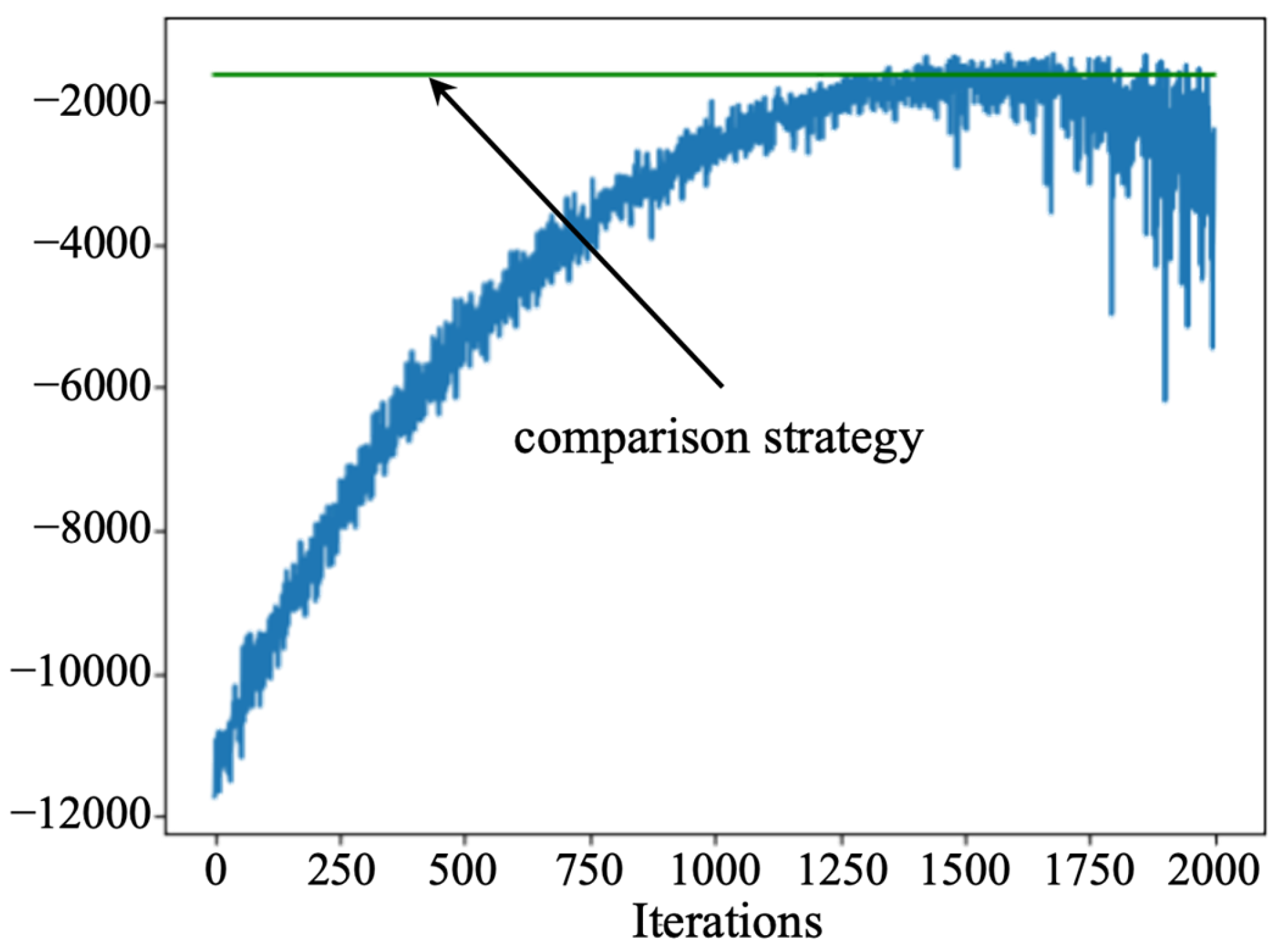
As shown in Table 3, the optimal maintenance schedule solved by the designed PPO algorithm has the lowest maintenance cost. The maintenance cost obtained by utilizing D3QN algorithm is the largest. To further analyze the reasons for this phenomenon, the training processes of the D3QN algorithm and the actor–critic algorithm are studied separately.
Figure 8 shows the training process of D3QN algorithm. As shown in Figure 8, the D3QN algorithm cannot obtain stable results within 1000 iterations, which is the maximum iterations of the designed PPO algorithm, and the performance shows a significant decline after 1500 rounds of iterations. Additionally, the maintenance cost obtained is slightly better than the comparison strategy, namely the control limit strategy, mentioned above.
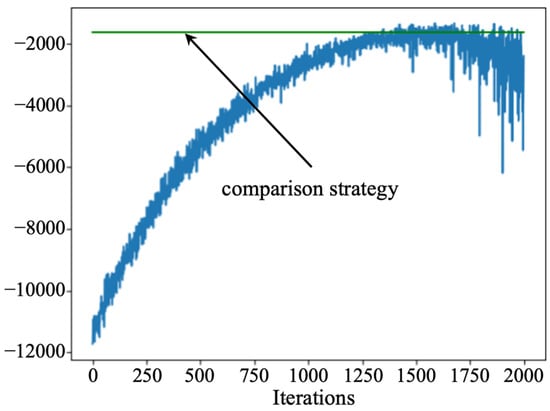
Figure 8.
Training process of the D3QN algorithm.
The training process of the actor–critic algorithm is shown in Figure 9. It can be found through Figure 9 that the maintenance cost obtained using the actor–critic algorithm is less than that of the comparison strategy. However, the performance of the actor–critic algorithm is unstable and tends to become trapped in local optimal solutions that cannot be jumped out of.
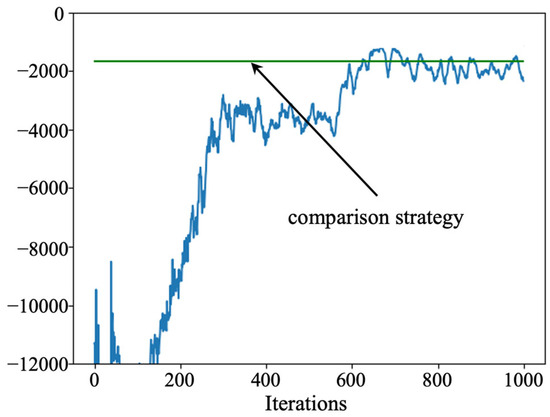
Figure 9.
Training process of the actor–critic algorithm.
In summary, the designed PPO algorithm can formulate maintenance schedule with the lowest cost, and it has the best stability compared to A and B. There may be several reasons for the better performance of the designed PPO algorithm:
- Sampling efficiency and sample utilization: The designed PPO algorithm uses the importance sampling technique in the optimization process, which can utilize the sampled data more efficiently and improve the efficiency of sample utilization. In contrast, the D3QN and actor–critic algorithms use the empirical playback mechanism, which usually requires more samples for training. Therefore, the PPO algorithm explores the solution space more fully under limited samples.
- Optimization strategy: the designed PPO is trained to update the parameters based on the policy gradient, and the final policy network gives the probability that an action takes a value. In contrast, the D3QN and actor–critic algorithms rely on estimating the value function and returning a determined action based on the value function. The probability of error is greater when estimating the value network, which is circumvented by the PPO algorithm.
- Algorithm stability: The tailored PPO algorithm is designed with a clip function, which can be the difference between the old and new policies within a certain range can effectively control the magnitude of the policy update, thus improving the stability of the algorithm. In contrast, D3QN and actor–critic algorithms may face overfitting or underfitting when dealing with complex environments and have lower training stability.
5.3. Implications for Practitioners
The proposed predictive maintenance strategy and optimization model for the no-wait production machine–robot collaborative environment have several important implications for practitioners in the manufacturing industry, particularly in the steel production sector.
- Enhanced Maintenance Planning and Scheduling: Practitioners can leverage the proposed system-level predictive maintenance model to optimize their maintenance planning and scheduling processes. By accounting for both degradation and sudden failure modes, the model enables a more precise prediction of equipment failures, thereby facilitating proactive maintenance actions. This not only reduces unplanned downtime but also minimizes production losses.
- Improved Cost Control and Financial Sustainability: The economic dependency among machines and robots within the production system is a key aspect of the proposed model. By optimizing maintenance schedules considering the interdependencies, practitioners can realize cost savings by scheduling joint maintenance activities. This approach is financially sustainable in the long run, reducing overall maintenance expenses and improving operational efficiency.
- Increased Flexibility and Responsiveness: The use of the PPO algorithm enables the development of adaptive maintenance policies that respond dynamically to the evolving production environment. Practitioners can incorporate this technology into their decision-making processes to quickly adapt to changes in production demands and equipment health status, ensuring continuous and stable operations.
- Enhanced System Reliability and Efficiency: The comprehensive model considers both structural and resource interdependencies within the production line, enabling a holistic approach to predictive maintenance. This in turn leads to improved system reliability and efficiency, reducing the likelihood of failures and minimizing the impact of equipment downtime.
- Data-Driven Decision-Making: The proposed strategy relies heavily on historical maintenance data and real-time equipment monitoring. Practitioners are encouraged to invest in data collection and analysis capabilities to continuously improve the predictive accuracy of the model. This data-driven approach ensures that maintenance decisions are informed and well-founded, leading to better outcomes.
In conclusion, the proposed predictive maintenance strategy and optimization model offer significant benefits for practitioners in the manufacturing industry. By addressing the complexities of no-wait production systems and incorporating the intricacies of machine–robot collaboration, the model provides a practical and effective approach to im-proving system reliability, efficiency, and cost control.
6. Conclusions
In this paper, a novel predictive maintenance method was developed for the manufacturing system of production machines-robots collaborative with the no-wait production process, which utilized downtime opportunities between production batches. To develop a more rational maintenance schedule, hybrid failure modes and economic dependency were considered in the developed maintenance framework. On this basis, a system-level maintenance optimization model was constructed to minimize the total cost in the finite horizon. Moreover, a tailored PPO algorithm with the clip function was designed to obtain the optimal maintenance schedule. A comprehensive case study was constructed to validate the effectiveness of the developed method. The results show that if economic dependency was ignored, total maintenance costs could be misestimated to mislead manufacturers. In addition, the comparative results showed that the developed method maximized the utilization of the machine’s performance and thus reduced the total maintenance cost.
It is worth noting that there are several challenges that will be addressed in future work. (1) In this paper, the parameter of imperfect maintenance is assumed to be deterministic. A robust predictive maintenance model considering stochastic imperfect maintenance is realistic and interesting. (2) In practice, the number of repairpersons is limited; therefore, joint optimization of predictive maintenance and repairperson allocation will be investigated. (3) The constructed degradation models may not reflect the actual performance of production machines and robots. Therefore, the development of maintenance decision-making method based on the partially observable Markov decision process (POMDP) is an effective way to address this challenge.
Author Contributions
Methodology, validation, writing, B.H.; software, formal analysis, Z.C. (Zhaoxiang Chen) and M.Z.; supervision, conceptualization, methodology, validation, Z.C. (Zhen Chen) supervision, investigation, visualization, E.P. All authors have read and agreed to the published version of the manuscript.
Funding
This work is supported by Natural Science Foundation of Shanghai under Grant 23ZR1428100.
Data Availability Statement
The data presented in this study are available on request from the corresponding author. The data are not publicly available due to privacy or ethical restrictions.
Acknowledgments
The authors would like to thank the editor and anonymous referees for their careful work and remarkable comments, which helped to improve this manuscript substantially.
Conflicts of Interest
Author Bing Hu is employed by the Shanghai Baosight Software Co., Ltd.; the remaining authors declare that the research was conducted in the absence of any commercial or financial relationships that could be construed as a potential conflict of interest.
References
- Zonta, T.; Da Costa, C.A.; da Rosa Righi, R.; de Lima, M.J.; da Trindade, E.S.; Li, G.P. Predictive maintenance in the Industry 4.0: A systematic literature review. Comput. Ind. Eng. 2020, 150, 106889. [Google Scholar] [CrossRef]
- Carvalho, T.P.; Soares, F.A.; Vita, R.; Francisco, R.D.P.; Basto, J.P.; Alcalá, S.G.A. Systematic literature review of machine learning methods applied to predictive maintenance. Comput. Ind. Eng. 2019, 137, 106024. [Google Scholar] [CrossRef]
- Chauvet, F.; Proth, J.M.; Wardi, Y. Scheduling no-wait production with time windows and flexible processing times. IEEE Trans. Robot. 2001, 17, 60–69. [Google Scholar] [CrossRef]
- Yamada, T.; Nagano, M.; Miyata, H. Minimization of total tardiness in no-wait flowshop production systems with preventive maintenance. Int. J. Ind. Eng. Comput. 2021, 12, 415–426. [Google Scholar] [CrossRef]
- Wang, B.; Tao, F.; Fang, X.; Liu, C.; Liu, Y.; Freiheit, T. Smart manufacturing and intelligent manufacturing: A comparative review. Engineering 2021, 7, 738–757. [Google Scholar] [CrossRef]
- Zhong, R.Y.; Xu, X.; Klotz, E.; Newman, S.T. Intelligent manufacturing in the context of industry 4.0: A review. Engineering 2017, 3, 616–630. [Google Scholar] [CrossRef]
- Zhang, W.; Yang, D.; Wang, H. Data-driven methods for predictive maintenance of industrial equipment: A survey. IEEE Syst. J. 2019, 13, 2213–2227. [Google Scholar] [CrossRef]
- Aivaliotis, P.; Arkouli, Z.; Georgoulias, K.; Makris, S. Degradation curves integration in physics-based models: Towards the predictive maintenance of industrial robots. Rob. Comput. Integr. Manuf. 2021, 71, 102177. [Google Scholar] [CrossRef]
- Hu, J.; Wang, H.; Tang, H.K.; Kanazawa, T.; Gupta, C.; Farahat, A. Knowledge-enhanced reinforcement learning for multi-machine integrated production and maintenance scheduling. Comput. Ind. Eng. 2023, 185, 109631. [Google Scholar] [CrossRef]
- Karlsson, A.; Bekar, E.T.; Skoogh, A. Multi-Machine Gaussian Topic Modeling for Predictive Maintenance. IEEE Access 2021, 9, 100063–100080. [Google Scholar] [CrossRef]
- Wang, H.; Yan, Q.; Zhang, S. Integrated scheduling and flexible maintenance in deteriorating multi-state single machine system using a reinforcement learning approach. Adv. Eng. Inf. 2021, 49, 101339. [Google Scholar] [CrossRef]
- Shoorkand, H.D.; Nourelfath, M.; Hajji, A. A hybrid deep learning approach to integrate predictive maintenance and production planning for multi-state systems. J. Manuf. Syst. 2024, 74, 397–410. [Google Scholar] [CrossRef]
- Wang, Y.; Li, X.; Chen, J.; Liu, Y. A condition-based maintenance policy for multi-component systems subject to stochastic and economic dependencies. Reliab. Eng. Syst. Saf. 2022, 219, 108174. [Google Scholar] [CrossRef]
- Zhou, Y.; Lin, T.R.; Sun, Y.; Ma, L. Maintenance optimisation of a parallel-series system with stochastic and economic dependence under limited maintenance capacity. Reliab. Eng. Syst. Saf. 2016, 155, 137–146. [Google Scholar] [CrossRef]
- Deep, A.; Zhou, S.; Veeramani, D. A data-driven recurrent event model for system degradation with imperfect maintenance actions. IISE Trans. 2021, 54, 271–285. [Google Scholar] [CrossRef]
- Mai, Y.; Xue, J.; Wu, B. Optimal maintenance policy for systems with environment-modulated degradation and random shocks considering imperfect maintenance. Reliab. Eng. Syst. Saf. 2023, 240, 109597. [Google Scholar] [CrossRef]
- Zhu, W.; Fouladirad, M.; Bérenguer, C. A multi-level maintenance policy for a multi-component and multifailure mode system with two independent failure modes. Reliab. Eng. Syst. Saf. 2016, 153, 50–63. [Google Scholar] [CrossRef]
- Chen, Z.; Chen, Z.; Zhou, D.; Xia, T.; Pan, E. Opportunistic maintenance optimization of continuous process manufacturing systems considering imperfect maintenance with epistemic uncertainty. J. Manuf. Syst. 2023, 71, 406–420. [Google Scholar] [CrossRef]
- Zhang, L.; Chen, X.; Khatab, A.; An, Y. Optimizing imperfect preventive maintenance in multi-component repairable systems under s-dependent competing risks. Reliab. Eng. Syst. Saf. 2022, 219, 108177. [Google Scholar] [CrossRef]
- Jianhui, D.; Yanyan, L.; Jine, H.; Jia, H. Maintenance Decision Optimization of Multi-State System Considering Imperfect Maintenance. Ind. Eng. Innov. Manag. 2022, 5, 16–24. [Google Scholar]
- Mullor, R.; Mulero, J.; Trottini, M. A modelling approach to optimal imperfect maintenance of repairable equipment with multiple failure modes. Comput. Ind. Eng. 2019, 128, 24–31. [Google Scholar] [CrossRef]
- Sharifi, M.; Taghipour, S. Optimal production and maintenance scheduling for a degrading multi-failure modes single-machine production environment. Appl. Soft Comput. 2021, 106, 107312. [Google Scholar] [CrossRef]
- Zheng, R.; Makis, V. Optimal condition-based maintenance with general repair and two dependent failure modes. Comput. Ind. Eng. 2020, 141, 106322. [Google Scholar] [CrossRef]
- Qiu, Q.; Cui, L.; Gao, H. Availability and maintenance modelling for systems subject to multiple failure modes. Comput. Ind. Eng. 2017, 108, 192–198. [Google Scholar] [CrossRef]
- Liu, P.; Wang, G. Optimal preventive maintenance policies for products with multiple failure modes after geometric warranty expiry. Commun. Stat.-Theory Methods 2023, 52, 8794–8813. [Google Scholar] [CrossRef]
- Qi, F.Q.; Yang, H.Q.; Wei, L.; Shu, X.T. Preventive maintenance policy optimization for a weighted k-out-of-n: G system using the survival signature. Reliab. Eng. Syst. Saf. 2024, 249, 110247. [Google Scholar] [CrossRef]
- Patra, P.; Kumar, U.K.D. Opportunistic and delayed maintenance as strategies for sustainable maintenance practices. Int. J. Qual. Reliab. Manag. 2024. ahead-of-print. [Google Scholar] [CrossRef]
- Chen, Z.; Zhou, D.; Xia, T.B.; Pan, E.S. Online unsupervised optimization framework for machine performance assessment based on distance metric learning. Mech. Syst. Signal Process. 2024, 206, 110883. [Google Scholar] [CrossRef]
- He, Y.H.; Gu, C.C.; Chen, Z.X.; Han, X. Integrated predictive maintenance strategy for manufacturing systems by combining quality control and mission reliability analysis. Int. J. Prod. Res. 2017, 55, 5841–5862. [Google Scholar] [CrossRef]
- Yuan, H.; Ni, J.; Hu, J.B. A centralised training algorithm with D3QN for scalable regular unmanned ground vehicle formation maintenance. IET Intell. Transp. Syst. 2021, 15, 562–572. [Google Scholar] [CrossRef]
- Liu, Y.; Chen, Y.M.; Jiang, T. Dynamic selective maintenance optimization for multi-state systems over a finite horizon: A deep reinforcement learning approach. Eur. J. Oper. Res. 2020, 283, 166–181. [Google Scholar] [CrossRef]
Disclaimer/Publisher’s Note: The statements, opinions and data contained in all publications are solely those of the individual author(s) and contributor(s) and not of MDPI and/or the editor(s). MDPI and/or the editor(s) disclaim responsibility for any injury to people or property resulting from any ideas, methods, instructions or products referred to in the content. |
© 2024 by the authors. Licensee MDPI, Basel, Switzerland. This article is an open access article distributed under the terms and conditions of the Creative Commons Attribution (CC BY) license (https://creativecommons.org/licenses/by/4.0/).


