
System-Level Predictive Maintenance Optimization for No-Wait Production Machine–Robot Collaborative Environment under Economic Dependency and Hybrid Fault Mode


Abstract
:1. Introduction
- (1)
- We present a novel predictive maintenance strategy that specifically addresses economic dependency within a no-wait production system, where machines and robots operate in a collaborative yet financially interlinked environment. This approach provides a more nuanced understanding of maintenance costs and benefits, leading to more informed decision-making.
- (2)
- The study introduces a sophisticated method for modeling equipment failure behavior that encompasses hybrid fault modes. This method enhances the predictive maintenance process by offering a more detailed and realistic representation of potential equipment failures, thereby improving the preemptive actions taken.
- (3)
- By employing a proximal policy optimization (PPO) algorithm, the research navigates the complexities of system-level maintenance optimization in a machine–robot collaborative setting. The PPO algorithm’s application allows for the development of adaptive maintenance policies that respond to the dynamic and interconnected nature of the production environment.
- (4)
- The findings establish a new benchmark for predictive maintenance in industrial applications, particularly in steel production, where the integration of economic factors and predictive analytics results in a strategy that is both scientifically sound and operationally efficient, setting a precedent for future research and industry practices.
2. Predictive Maintenance Strategy Formulation for NWPMRCMP
2.1. Problem Statement
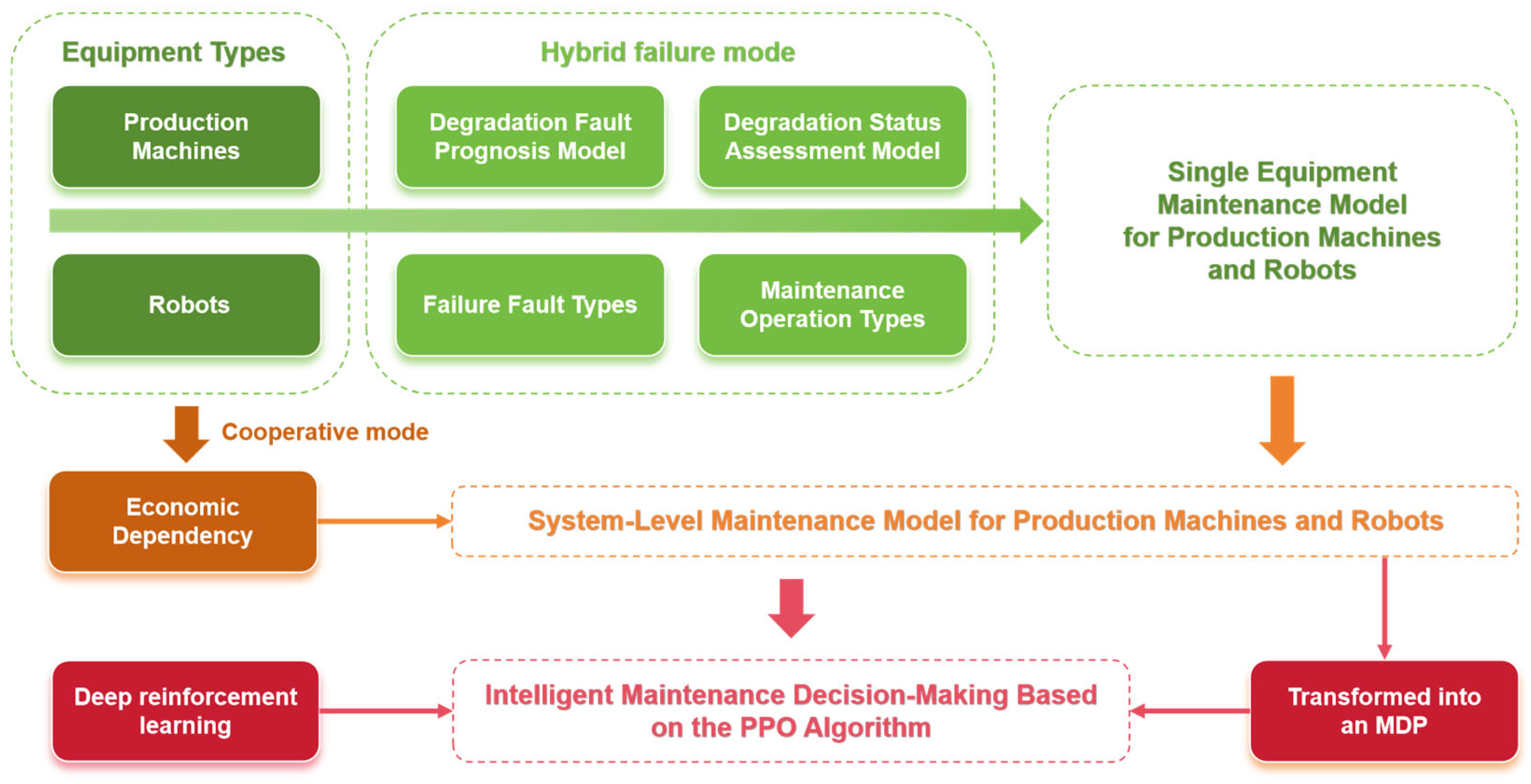
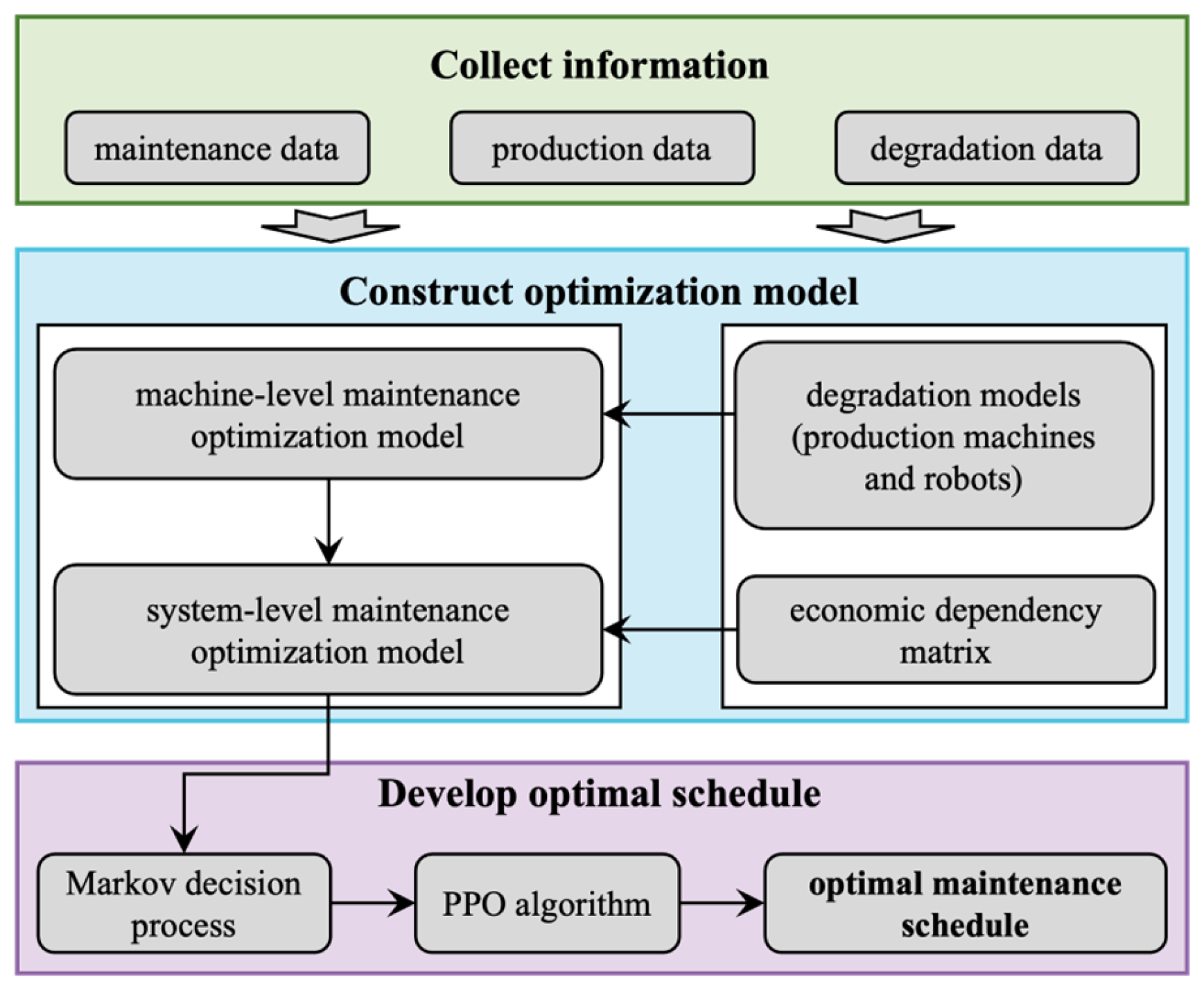
2.2. Overall Framework of the Proposed Method
3. System-Level Collaborative Predictive Maintenance Optimization Model
3.1. Machine-Level Maintenance Model under Hybrid Fault Mode
3.2. System-Level Maintenance Optimization Model Considering Economic Dependency
4. Optimization Algorithm Based on DRL
| Algorithm 1. Pseudocode of the PPO Algorithm |
| Input Parameters: State Space , Reward Space , Action Space , Learning rate, Number of network update steps , etc. |
| Initialization: policy network , value network , Advantage function estimation parameters, optimization parameters. |
| For each training epoch |
| Randomly initialize the state , create a new dataset |
| For each time step |
| Perform the current action given by the policy network |
| Execute the action , obtain the current reward and the next system state |
| Store the sample in the dataset |
| End |
| For each sample |
| Calculate the predicted value of the next state: |
| Calculate the target value: |
| Calculate the temporal difference error: |
| End |
| Calculate the advantage function in reverse order: |
| Calculate the ratio of the new to old policy: |
| Calculate the policy network loss function: |
| Calculate the value network loss function: |
| Back propagate to update the parameters of the policy network and the value network . |
| Update the parameters of the old policy network: . |
| End |
| Output Results: |
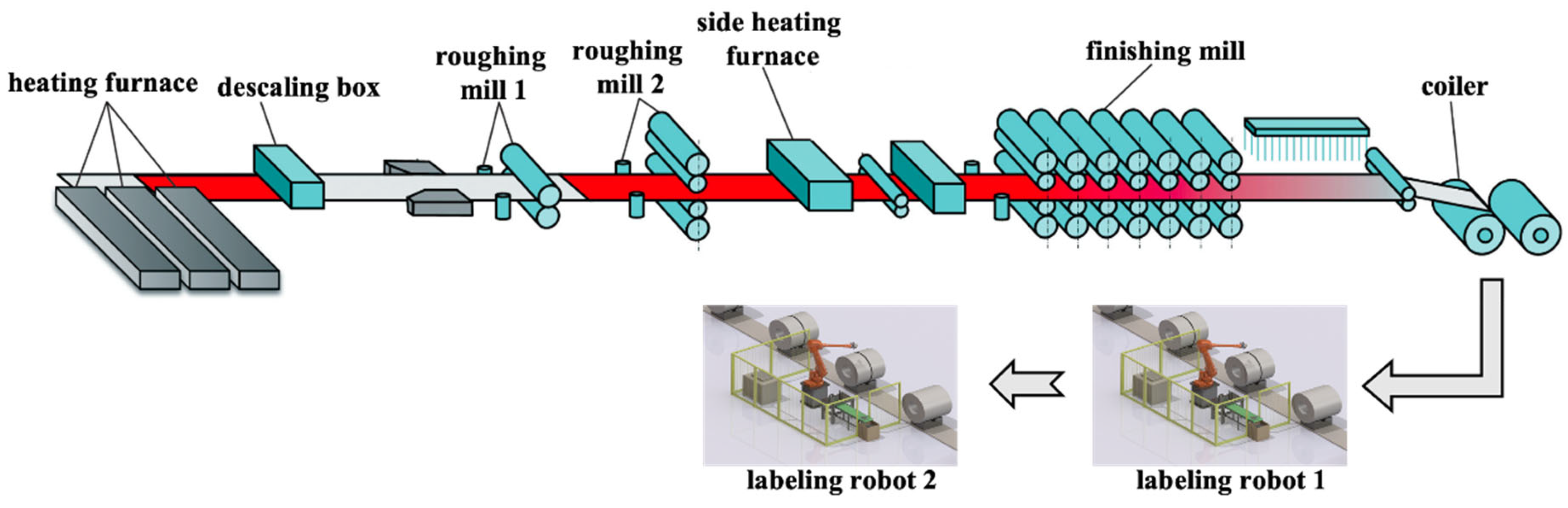
5. Case Study
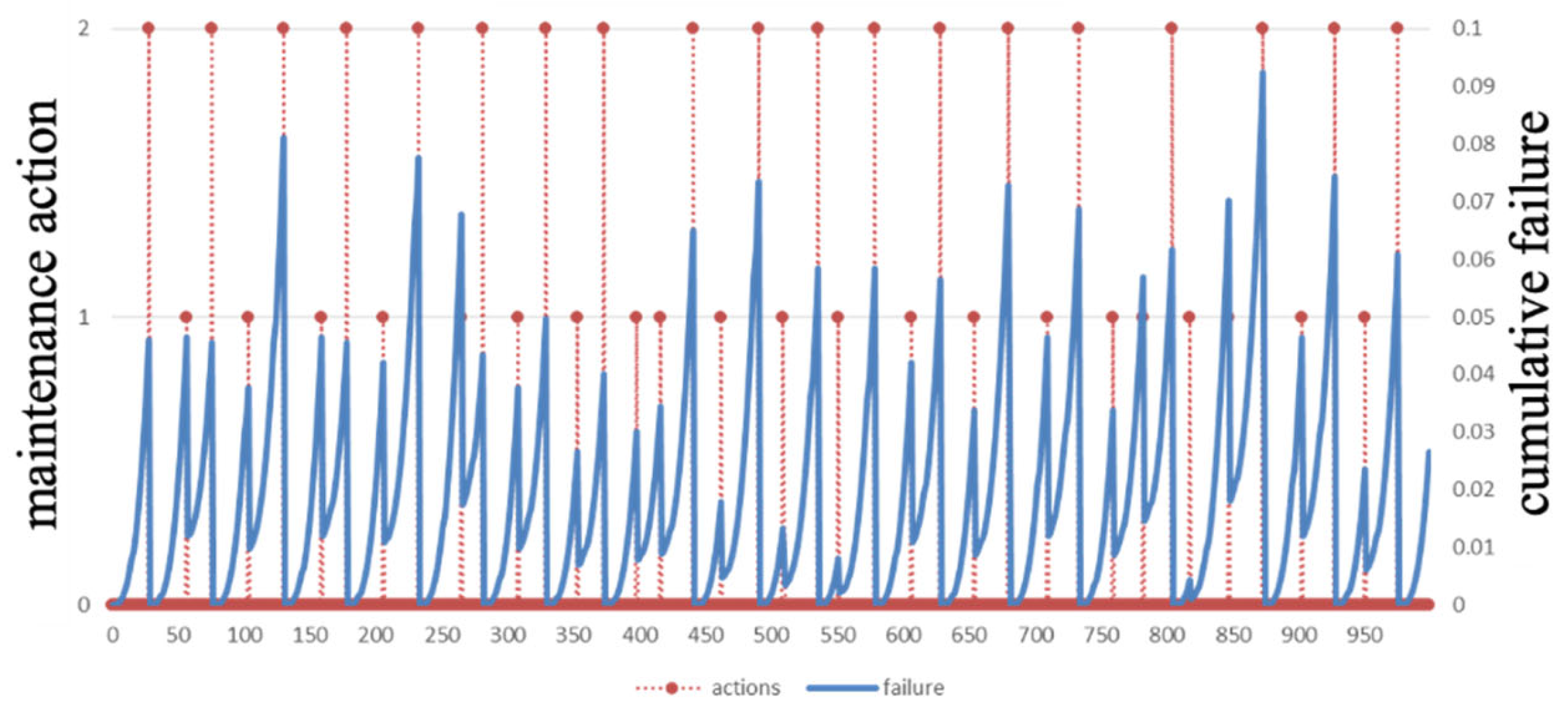
5.1. Optimal Maintenance Policy
5.2. Discussion
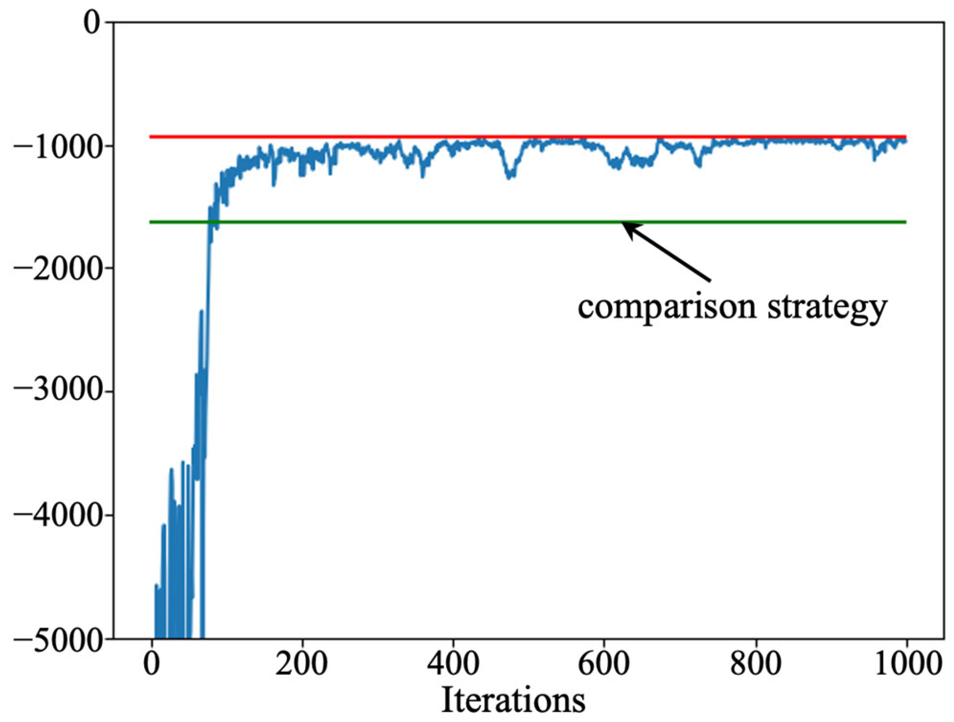
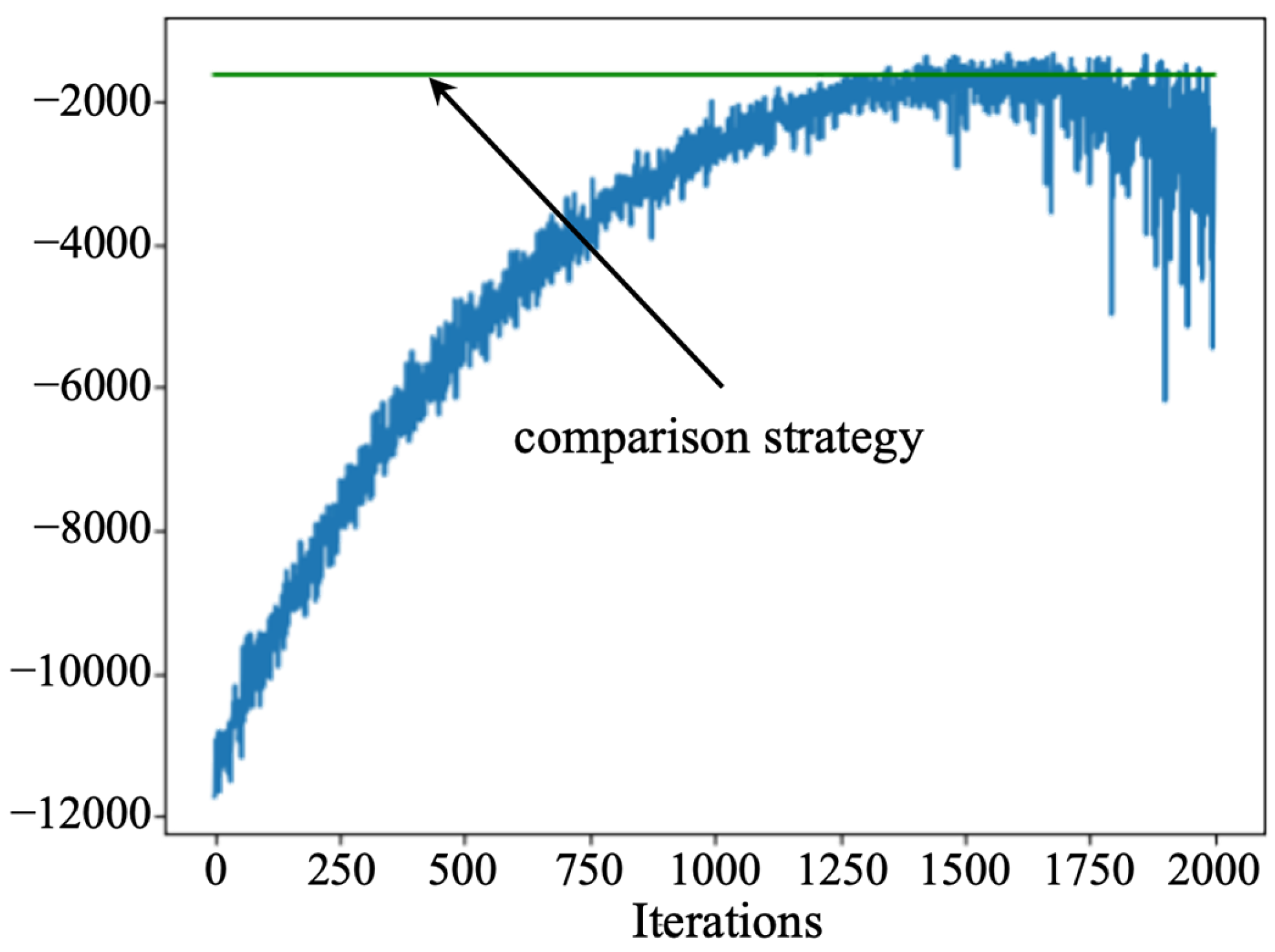
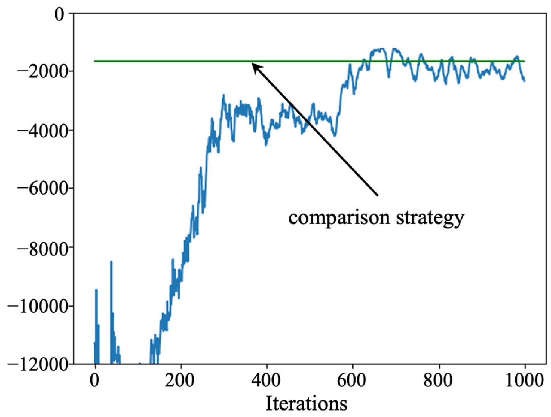
- Sampling efficiency and sample utilization: The designed PPO algorithm uses the importance sampling technique in the optimization process, which can utilize the sampled data more efficiently and improve the efficiency of sample utilization. In contrast, the D3QN and actor–critic algorithms use the empirical playback mechanism, which usually requires more samples for training. Therefore, the PPO algorithm explores the solution space more fully under limited samples.
- Optimization strategy: the designed PPO is trained to update the parameters based on the policy gradient, and the final policy network gives the probability that an action takes a value. In contrast, the D3QN and actor–critic algorithms rely on estimating the value function and returning a determined action based on the value function. The probability of error is greater when estimating the value network, which is circumvented by the PPO algorithm.
- Algorithm stability: The tailored PPO algorithm is designed with a clip function, which can be the difference between the old and new policies within a certain range can effectively control the magnitude of the policy update, thus improving the stability of the algorithm. In contrast, D3QN and actor–critic algorithms may face overfitting or underfitting when dealing with complex environments and have lower training stability.
5.3. Implications for Practitioners
- Enhanced Maintenance Planning and Scheduling: Practitioners can leverage the proposed system-level predictive maintenance model to optimize their maintenance planning and scheduling processes. By accounting for both degradation and sudden failure modes, the model enables a more precise prediction of equipment failures, thereby facilitating proactive maintenance actions. This not only reduces unplanned downtime but also minimizes production losses.
- Improved Cost Control and Financial Sustainability: The economic dependency among machines and robots within the production system is a key aspect of the proposed model. By optimizing maintenance schedules considering the interdependencies, practitioners can realize cost savings by scheduling joint maintenance activities. This approach is financially sustainable in the long run, reducing overall maintenance expenses and improving operational efficiency.
- Increased Flexibility and Responsiveness: The use of the PPO algorithm enables the development of adaptive maintenance policies that respond dynamically to the evolving production environment. Practitioners can incorporate this technology into their decision-making processes to quickly adapt to changes in production demands and equipment health status, ensuring continuous and stable operations.
- Enhanced System Reliability and Efficiency: The comprehensive model considers both structural and resource interdependencies within the production line, enabling a holistic approach to predictive maintenance. This in turn leads to improved system reliability and efficiency, reducing the likelihood of failures and minimizing the impact of equipment downtime.
- Data-Driven Decision-Making: The proposed strategy relies heavily on historical maintenance data and real-time equipment monitoring. Practitioners are encouraged to invest in data collection and analysis capabilities to continuously improve the predictive accuracy of the model. This data-driven approach ensures that maintenance decisions are informed and well-founded, leading to better outcomes.
6. Conclusions
Author Contributions
Funding
Data Availability Statement
Acknowledgments
Conflicts of Interest
References
- Zonta, T.; Da Costa, C.A.; da Rosa Righi, R.; de Lima, M.J.; da Trindade, E.S.; Li, G.P. Predictive maintenance in the Industry 4.0: A systematic literature review. Comput. Ind. Eng. 2020, 150, 106889. [Google Scholar] [CrossRef]
- Carvalho, T.P.; Soares, F.A.; Vita, R.; Francisco, R.D.P.; Basto, J.P.; Alcalá, S.G.A. Systematic literature review of machine learning methods applied to predictive maintenance. Comput. Ind. Eng. 2019, 137, 106024. [Google Scholar] [CrossRef]
- Chauvet, F.; Proth, J.M.; Wardi, Y. Scheduling no-wait production with time windows and flexible processing times. IEEE Trans. Robot. 2001, 17, 60–69. [Google Scholar] [CrossRef]
- Yamada, T.; Nagano, M.; Miyata, H. Minimization of total tardiness in no-wait flowshop production systems with preventive maintenance. Int. J. Ind. Eng. Comput. 2021, 12, 415–426. [Google Scholar] [CrossRef]
- Wang, B.; Tao, F.; Fang, X.; Liu, C.; Liu, Y.; Freiheit, T. Smart manufacturing and intelligent manufacturing: A comparative review. Engineering 2021, 7, 738–757. [Google Scholar] [CrossRef]
- Zhong, R.Y.; Xu, X.; Klotz, E.; Newman, S.T. Intelligent manufacturing in the context of industry 4.0: A review. Engineering 2017, 3, 616–630. [Google Scholar] [CrossRef]
- Zhang, W.; Yang, D.; Wang, H. Data-driven methods for predictive maintenance of industrial equipment: A survey. IEEE Syst. J. 2019, 13, 2213–2227. [Google Scholar] [CrossRef]
- Aivaliotis, P.; Arkouli, Z.; Georgoulias, K.; Makris, S. Degradation curves integration in physics-based models: Towards the predictive maintenance of industrial robots. Rob. Comput. Integr. Manuf. 2021, 71, 102177. [Google Scholar] [CrossRef]
- Hu, J.; Wang, H.; Tang, H.K.; Kanazawa, T.; Gupta, C.; Farahat, A. Knowledge-enhanced reinforcement learning for multi-machine integrated production and maintenance scheduling. Comput. Ind. Eng. 2023, 185, 109631. [Google Scholar] [CrossRef]
- Karlsson, A.; Bekar, E.T.; Skoogh, A. Multi-Machine Gaussian Topic Modeling for Predictive Maintenance. IEEE Access 2021, 9, 100063–100080. [Google Scholar] [CrossRef]
- Wang, H.; Yan, Q.; Zhang, S. Integrated scheduling and flexible maintenance in deteriorating multi-state single machine system using a reinforcement learning approach. Adv. Eng. Inf. 2021, 49, 101339. [Google Scholar] [CrossRef]
- Shoorkand, H.D.; Nourelfath, M.; Hajji, A. A hybrid deep learning approach to integrate predictive maintenance and production planning for multi-state systems. J. Manuf. Syst. 2024, 74, 397–410. [Google Scholar] [CrossRef]
- Wang, Y.; Li, X.; Chen, J.; Liu, Y. A condition-based maintenance policy for multi-component systems subject to stochastic and economic dependencies. Reliab. Eng. Syst. Saf. 2022, 219, 108174. [Google Scholar] [CrossRef]
- Zhou, Y.; Lin, T.R.; Sun, Y.; Ma, L. Maintenance optimisation of a parallel-series system with stochastic and economic dependence under limited maintenance capacity. Reliab. Eng. Syst. Saf. 2016, 155, 137–146. [Google Scholar] [CrossRef]
- Deep, A.; Zhou, S.; Veeramani, D. A data-driven recurrent event model for system degradation with imperfect maintenance actions. IISE Trans. 2021, 54, 271–285. [Google Scholar] [CrossRef]
- Mai, Y.; Xue, J.; Wu, B. Optimal maintenance policy for systems with environment-modulated degradation and random shocks considering imperfect maintenance. Reliab. Eng. Syst. Saf. 2023, 240, 109597. [Google Scholar] [CrossRef]
- Zhu, W.; Fouladirad, M.; Bérenguer, C. A multi-level maintenance policy for a multi-component and multifailure mode system with two independent failure modes. Reliab. Eng. Syst. Saf. 2016, 153, 50–63. [Google Scholar] [CrossRef]
- Chen, Z.; Chen, Z.; Zhou, D.; Xia, T.; Pan, E. Opportunistic maintenance optimization of continuous process manufacturing systems considering imperfect maintenance with epistemic uncertainty. J. Manuf. Syst. 2023, 71, 406–420. [Google Scholar] [CrossRef]
- Zhang, L.; Chen, X.; Khatab, A.; An, Y. Optimizing imperfect preventive maintenance in multi-component repairable systems under s-dependent competing risks. Reliab. Eng. Syst. Saf. 2022, 219, 108177. [Google Scholar] [CrossRef]
- Jianhui, D.; Yanyan, L.; Jine, H.; Jia, H. Maintenance Decision Optimization of Multi-State System Considering Imperfect Maintenance. Ind. Eng. Innov. Manag. 2022, 5, 16–24. [Google Scholar]
- Mullor, R.; Mulero, J.; Trottini, M. A modelling approach to optimal imperfect maintenance of repairable equipment with multiple failure modes. Comput. Ind. Eng. 2019, 128, 24–31. [Google Scholar] [CrossRef]
- Sharifi, M.; Taghipour, S. Optimal production and maintenance scheduling for a degrading multi-failure modes single-machine production environment. Appl. Soft Comput. 2021, 106, 107312. [Google Scholar] [CrossRef]
- Zheng, R.; Makis, V. Optimal condition-based maintenance with general repair and two dependent failure modes. Comput. Ind. Eng. 2020, 141, 106322. [Google Scholar] [CrossRef]
- Qiu, Q.; Cui, L.; Gao, H. Availability and maintenance modelling for systems subject to multiple failure modes. Comput. Ind. Eng. 2017, 108, 192–198. [Google Scholar] [CrossRef]
- Liu, P.; Wang, G. Optimal preventive maintenance policies for products with multiple failure modes after geometric warranty expiry. Commun. Stat.-Theory Methods 2023, 52, 8794–8813. [Google Scholar] [CrossRef]
- Qi, F.Q.; Yang, H.Q.; Wei, L.; Shu, X.T. Preventive maintenance policy optimization for a weighted k-out-of-n: G system using the survival signature. Reliab. Eng. Syst. Saf. 2024, 249, 110247. [Google Scholar] [CrossRef]
- Patra, P.; Kumar, U.K.D. Opportunistic and delayed maintenance as strategies for sustainable maintenance practices. Int. J. Qual. Reliab. Manag. 2024. ahead-of-print. [Google Scholar] [CrossRef]
- Chen, Z.; Zhou, D.; Xia, T.B.; Pan, E.S. Online unsupervised optimization framework for machine performance assessment based on distance metric learning. Mech. Syst. Signal Process. 2024, 206, 110883. [Google Scholar] [CrossRef]
- He, Y.H.; Gu, C.C.; Chen, Z.X.; Han, X. Integrated predictive maintenance strategy for manufacturing systems by combining quality control and mission reliability analysis. Int. J. Prod. Res. 2017, 55, 5841–5862. [Google Scholar] [CrossRef]
- Yuan, H.; Ni, J.; Hu, J.B. A centralised training algorithm with D3QN for scalable regular unmanned ground vehicle formation maintenance. IET Intell. Transp. Syst. 2021, 15, 562–572. [Google Scholar] [CrossRef]
- Liu, Y.; Chen, Y.M.; Jiang, T. Dynamic selective maintenance optimization for multi-state systems over a finite horizon: A deep reinforcement learning approach. Eur. J. Oper. Res. 2020, 283, 166–181. [Google Scholar] [CrossRef]


| Parameters | Value |
|---|---|
| Number of iterations | 1000 |
| Optimizer | Adam |
| Activation function | ReLu |
| Number of hidden layers | 1 |
| Number of neurons in the hidden layer | 16 |
| Initial learning rate of policy network | 0.001 |
| Initial learning rate of value network | 0.01 |
| Smoothing factor of advantage function | 0.95 |
| Truncation parameter of clip function | 0.2 |
| Maintenance Cost | |
|---|---|
| Economic dependency | 900.8815 |
| Non-economic dependency | 1083.5468 |
| Algorithms | Maintenance Cost |
|---|---|
| PPO | 900.8815 |
| D3QN | 1336.3222 |
| Actor-Critic | 1154.8539 |
Disclaimer/Publisher’s Note: The statements, opinions and data contained in all publications are solely those of the individual author(s) and contributor(s) and not of MDPI and/or the editor(s). MDPI and/or the editor(s) disclaim responsibility for any injury to people or property resulting from any ideas, methods, instructions or products referred to in the content. |
© 2024 by the authors. Licensee MDPI, Basel, Switzerland. This article is an open access article distributed under the terms and conditions of the Creative Commons Attribution (CC BY) license (https://creativecommons.org/licenses/by/4.0/).
Share and Cite
Hu, B.; Chen, Z.; Zhen, M.; Chen, Z.; Pan, E. System-Level Predictive Maintenance Optimization for No-Wait Production Machine–Robot Collaborative Environment under Economic Dependency and Hybrid Fault Mode. Processes 2024, 12, 1690. https://doi.org/10.3390/pr12081690
Hu B, Chen Z, Zhen M, Chen Z, Pan E. System-Level Predictive Maintenance Optimization for No-Wait Production Machine–Robot Collaborative Environment under Economic Dependency and Hybrid Fault Mode. Processes. 2024; 12(8):1690. https://doi.org/10.3390/pr12081690
Chicago/Turabian StyleHu, Bing, Zhaoxiang Chen, Mengzi Zhen, Zhen Chen, and Ershun Pan. 2024. "System-Level Predictive Maintenance Optimization for No-Wait Production Machine–Robot Collaborative Environment under Economic Dependency and Hybrid Fault Mode" Processes 12, no. 8: 1690. https://doi.org/10.3390/pr12081690
APA StyleHu, B., Chen, Z., Zhen, M., Chen, Z., & Pan, E. (2024). System-Level Predictive Maintenance Optimization for No-Wait Production Machine–Robot Collaborative Environment under Economic Dependency and Hybrid Fault Mode. Processes, 12(8), 1690. https://doi.org/10.3390/pr12081690