Abstract
Construction projects require concurrent consideration of the three major objectives of construction period, cost, and quality. To address the multi-objective optimization issues of construction projects, mathematical models of construction period, quality, and cost are established, respectively, and multi-objective optimization models are constructed for different construction objectives. A hybrid optimization method combining an improved genetic algorithm (GA) with a time-varying mutation rate and a particle swarm algorithm (PSO) is proposed to optimize construction projects, which overcomes the shortcomings of the original GA and improves the global optimality and stability of results. Various construction projects were considered, and different construction objectives were analyzed individually. Finally, an uncertainty analysis is developed for the proposed GA-PSO algorithm and compared with GA and PSO. The results indicate that the proposed hybrid approach outperforms the PSO and GA algorithms in providing a better and more stable multi-objective optimized construction solution, with performance improvements of 4.3–8.5% and volatility reductions of 37.5–64.4%. This provides a reference for the optimal design of wind farms, buildings, and other construction projects.
1. Introduction
The construction process of subways, buildings, airports, and other projects not only has a long period and huge cost but also has plenty of risks; hence, it is necessary to consider the three major objectives of construction period, cost, and quality to realize the shortest construction period, the lowest construction cost, and the highest project quality [1]. For example, to put the subway into operation as soon as possible, some cities will accelerate the construction period, which will easily lead to an increase in costs and frequent accidents; while if excessive attention is paid to the quality of the subway construction process, it will increase the corresponding construction period and costs. Therefore, achieving multi-objective optimization of construction period, cost, and quality is crucial for construction project managers. As a result, numerous scholars have centered their research on multi-objective optimization of construction projects [2,3,4].
Multi-objective optimization algorithms can be classified into two broad classes: exact algorithms and heuristics [5]. By formulating multi-objective programs as linear programs, exact algorithms can solve optimization problems with exponential computational complexity [6]. As pointed out by Ameri et al. [7], France-Mensah et al. [8], and Sun et al. [9], scalarization methods can leverage existing techniques or platforms to solve multi-objective optimization problems, resulting in accurate solutions. However, larger optimization problems have more complicated solution spaces and many constraints, making exact algorithms slower and difficult to implement. Heuristic algorithms are inspired by the characteristics of problems and constructed based on specific mathematical rules, which usually produce only a fixed number of suboptimal solutions, e.g., greedy algorithm [10]. Their computational time is short, but optimality is not guaranteed. Metaheuristic algorithms do not rely on problem characteristics but rather obtain near-optimal solutions by successive iterations of randomized algorithms and local search. It explores and exploits the search space by combining different intelligent concepts and uses a learning strategy to organize the information to efficiently find near-optimal solutions, such as genetic algorithm (GA) [11], particle swarm optimization (PSO) [12], evolutionary algorithm, random search, etc.
GA is an evolutionary algorithm that mimics the natural law of survival of the fittest and has been widely used to solve optimization solutions for problems of varying complexity, including simple linear optimization and combinatorial optimization at the project level [13]. It uses binary coding to randomly generate an initial population and then mimics mating, mutation, and selection in nature by iterating to produce a more optimal population, which, in turn, generates a new feasible solution. Sindi et al. [14] solved a multi-objective optimization problem for pavement construction using GA by transforming it into a single objective function. Santos et al. [15] incorporated a local search-based algorithm into GA to enhance the overall efficiency. Some scholars adopted non-dominated sorting GAs (NSGA-II) to obtain Pareto optimal solutions [16,17,18]. However, the more objectives are considered, the more difficult it is to produce an overall solution. Even when a set of solutions is obtained, it is often difficult to interpret the optimization performance because each solution contains values associated with multiple objectives. Moreover, binary coding reduces the space of feasible solutions, and increasing the binary length makes the computation more intensive and time-consuming.
Compared to GA-based algorithms, PSO can break through the limitations of binary coding, thus finding more available solutions. PSO starts with a randomly generated set of particles, each representing a solution, and keeps updating these particles to get better solutions. Ahmed et al. [19] applied a binary multi-objective PSO with chaos methods for pavement maintenance management. Ji et al. [20] presented a hybrid method that combines the Markov chain and PSO to optimize pavement maintenance strategies. Nevertheless, PSO-based algorithms are prone to precociousness and falling into local optimality. Yang et al. [21] proposed an adaptive inertia-weighted PSO based on the optimized results of the GA stage for wind farm layout optimization. This approach can break through the low-resolution limitation of GA to quickly obtain the global optimum. However, the optimized results may be mainly determined by the GA.
This study aims to propose a hybrid approach for the optimization of construction projects based on improved GA and PSO (i.e., GA-PSO) to utilize the advantages of GA and PSO algorithms and to obtain solutions that are closer to the global optimum and more stable. The main contributions of this study are summarized as follows:
- (i)
- Mathematical models of the construction project period, cost, and quality were established, respectively, on the basis of which six optimization objectives were determined, forming six multi-objective optimization models of period–cost–quality.
- (ii)
- An improved GA with a time-varying mutation rate is proposed for the construction project for optimization, based on which PSO is used for further optimization to avoid falling into the local optimum and to improve the stability of performance.
- (iii)
- The performance of the proposed GA-PSO method has been thoroughly investigated using four different real construction projects with uncertainty analysis, and the results have been compared with other existing methods.
This paper is organized as follows: Section 2 introduces the methods for multi-objective optimization of construction projects. Section 3 presents case studies of construction project optimization, and Section 4 provides an in-depth discussion of the results. Finally, Section 5 summarizes the main conclusions of this study.
2. Methods for Multi-Objective Optimization of Construction Project
2.1. Flowchart
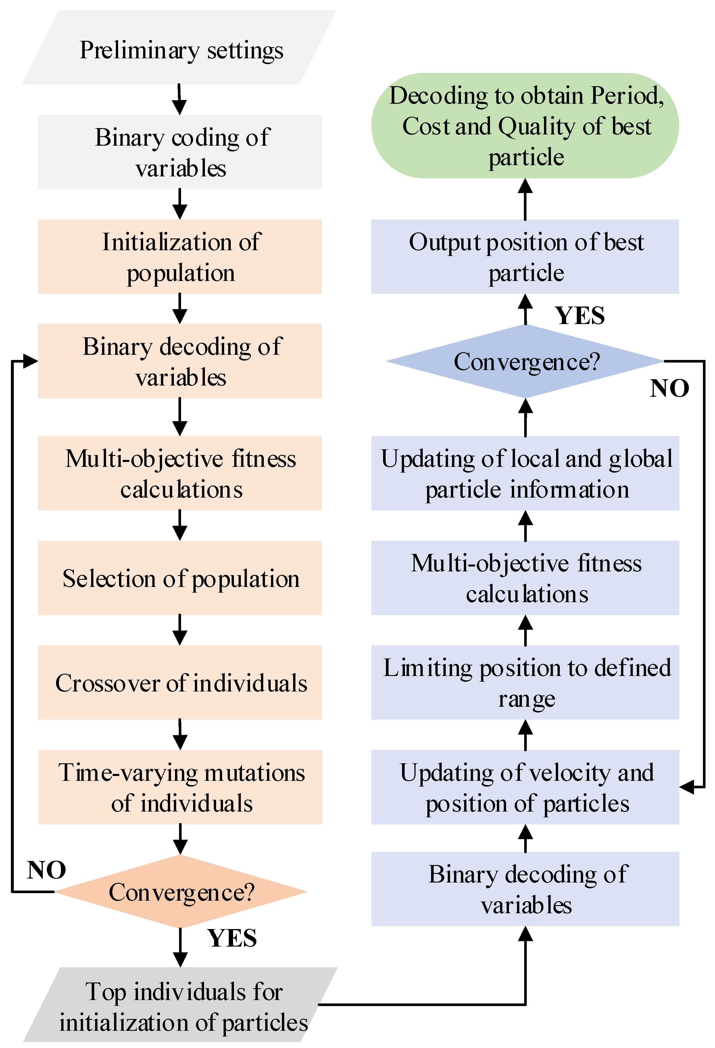
The proposed hybrid approach for multi-objective optimization of construction projects is shown in Figure 1.
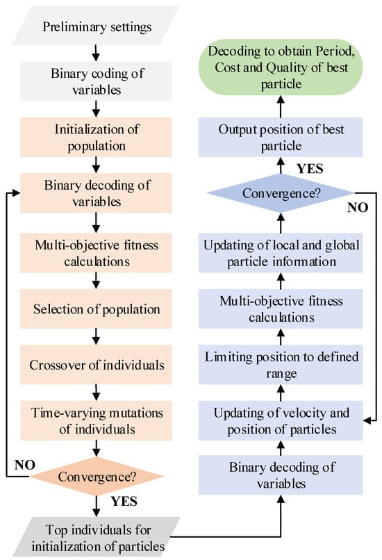
Figure 1.
Flowchart for multi-objective optimization of construction projects.
The improved GA can be utilized for multi-objective preliminary optimization through binary coding of construction variables, population initialization, binary decoding, multi-objective fitness calculation, population selection, individual crossover, individual mutation, etc. It is recommended to use the mutation rate over time to avoid falling into a local optimum. A few best-performing individuals are selected as initial particles for PSO with chaotic perturbations. Then, the PSO-based multi-objective optimization is completed sequentially by binary decoding, updating particle positions, constraining particles, multi-objective fitness calculation, and updating particle information. Finally, the best solution for a construction project can be obtained by decoding the optimal particle, as shown in the last two steps in Figure 1. The pseudo code for the proposed GA-PSO is shown in Algorithm 1, and the validation is performed by four different construction projects in Section 3.
| Algorithm 1: GA-PSO method |
| 1. Parameter setting. 2. Binary coding of variables. 3. Initialization of GA. 4. for i = 1:MaxIteration Decoding of binary variables. Multi-objective fitness calculation. Selection with roulette wheel selection method to obtain new individuals. Random crossover of individuals. Mutation of individuals with time-varying mutation rate. end 5. Obtain top individuals by GA. 6. Initialization of PSO by Binary decoding of variables. 7. for j = 1:MaxIteration Updating particles in terms of velocity and position. Limiting positions for particles. Multi-objective fitness calculation. Updating particles in terms of local and global information. end 8. Obtain the best particle. 9. Decoding of the best particle. |
2.2. Models
In multi-objective optimization of construction projects, three main parameters are considered, i.e., construction period, cost, and quality. Mathematical modeling of the three objectives is introduced in this section.
2.2.1. Construction Period Modeling
The total period of the construction project should be the sum of the periods of the processes on the “critical routes” in the network plan. Thus, the construction period can be calculated according to Equation (1).
where T denotes the construction period; n denotes the total number of construction processes; tj denotes the construction period of j th construction process; xi,j denotes the index variable, xi,j = 1 when j th process is contained in i th route in the network plan, otherwise xi,j = 0; and A denotes the set of feasible routes.
2.2.2. Cost Modeling
Construction costs for the project from the beginning of construction preparation to the end of the project throughout the construction process of all production costs, including direct costs and indirect costs. Direct costs are the costs incurred by the construction unit for the construction of the project, including labor, materials, machinery, etc., while indirect costs are the costs incurred by the construction unit for the management of the project, including salaries, depreciation of fixed assets, and repair costs, etc. Direct costs decrease over the construction period, while indirect costs increase over the construction period [22]. The function relationship between construction cost and construction period in Equation (2) can be obtained based on the parabolic hypothesis [23].
where C denotes the construction cost; and denotes the maximum and minimum construction period of j th construction process, respectively; and denotes the maximum and minimum direct construction cost of j th construction process, respectively; and and denotes the maximum and minimum direct construction cost of j th construction process, respectively.
2.2.3. Quality Modeling
The construction quality varies from one construction program to another due to the different construction methods, labor, and machinery used. Generally, the shorter the construction period required, the more difficult it is to ensure quality due to the need to rush; vice versa, the longer the construction period, the better the construction quality. The function relationship between construction quality and construction period in an equation can be obtained based on the parabolic hypothesis.
where Q denotes the construction quality; and denotes the maximum and minimum construction quality of j th construction process, respectively; and denotes the importance weighting factor of the j th process.
2.2.4. Multi-Objective Optimization Modeling
Multi-objective optimization aims to minimize the construction period, minimize the cost, and maximize the quality while the construction period, cost, and quality satisfy certain constraints, as described in Equations (4) and (5). Under such preconditions, a set of Pareto optimal solutions can be obtained using optimization algorithms such as NSGA-II, and the optimal solution can be decided by the decision-maker.
where Ttar and Ctar denote the maximum requirement of construction period and cost, respectively; and Qtar denotes the minimum requirement of construction quality.
For different construction projects, the decision-maker’s requirements for the three objectives vary. Thus, a set of Pareto optimal solutions may be difficult to interpret and select. To optimize the project comprehensively, the optimization objective functions of construction period, cost, and quality are weighted to establish a comprehensive optimization model of construction period–cost–quality, as shown in Equation (6).
where wT, wC and wQ denote the weights of the construction period, cost, and quality, respectively, and wT + wC + wQ = 1; T′, C′ and Q′ denote the dimensionless construction period, cost, and quality, respectively; Tmax and Tmin denote the maximum and minimum of the construction period, respectively; Cmax and Cmin denote the maximum and minimum of construction cost, respectively; and Qmax and Qmin denote the maximum and minimum of construction quality, respectively. Weights can be determined by the decision-maker based on different construction targets.
2.3. Optimization Methods
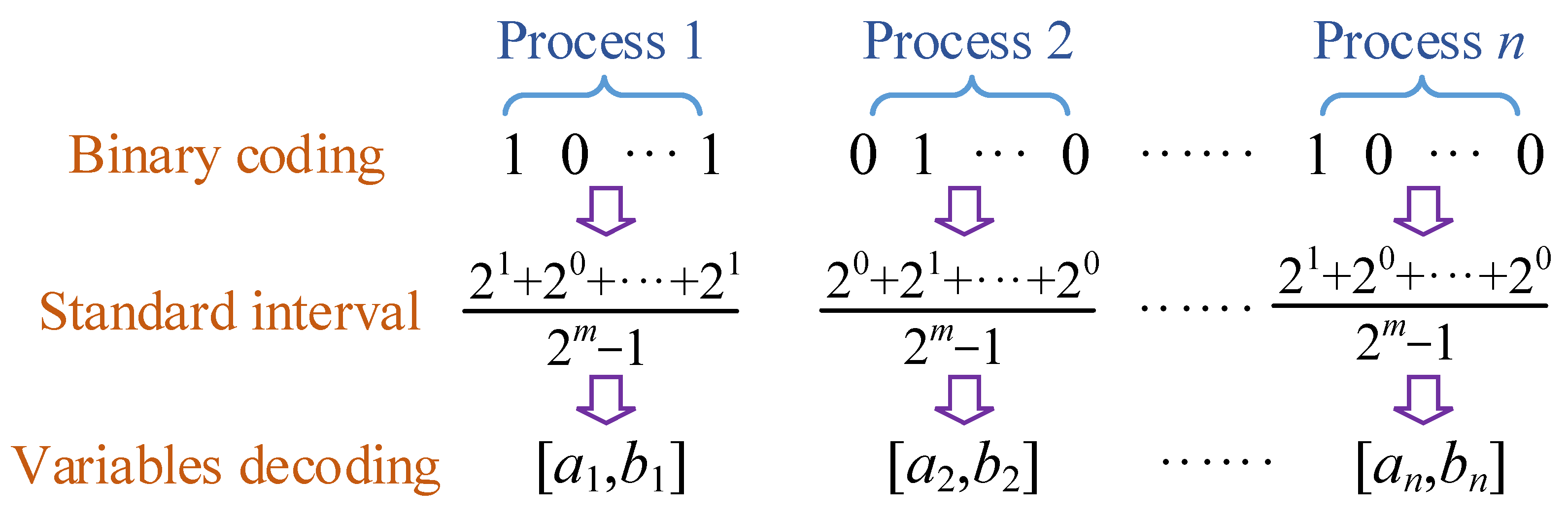
In this study, a hybrid GA-PSO method is proposed for multi-objective optimization of construction projects. GA solves optimization problems by mimicking nature’s eutrophication. Using binary coding to represent the construction duration of each process, cost and quality can be obtained according to Equations (2) and (3). Figure 2 displays the coding and decoding of the construction project, where m denotes the binary length, and a and b denote the lower and upper limits of the construction parameter, respectively. Each individual in the population is represented by a string of binary symbols. Optimal population is eventually obtained by repeated selection, crossover, and mutation of individuals.
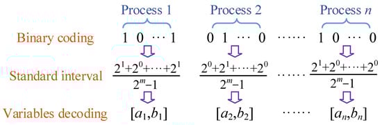
Figure 2.
Coding and decoding of a construction project based on genetic algorithm.
A variable mutation rate that varies linearly with the iteration steps is suggested to avoid it easily falling into local optimum within a few steps, as described in Equation (7).
where ri denotes the mutation rate at i th step; N1 denotes the maximum iteration step of GA; and rmax and rmin denote the maximum and minimum mutation rate, respectively.
The performance of GA optimization is affected by the binary length, and increasing the binary length will greatly enlarge the computation and be time-consuming. Here, the top 10 individuals in GA are chosen as the initial particles for PSO, where chaotic randomness is considered to find more feasible solutions. The principles of PSO are introduced in Equations (8)–(10).
where wj denotes the proposed time-varying inertial factor at j th step; w1 and w2 denote the initial and final inertial factor, respectively; N2 denotes the maximum iteration step of PSO; vi and xi denotes the velocity and position of i th particle, respectively; c1 and c2 denote the individual learning factor and social learning factor, respectively; r1 and r2 denote random number in the interval [0, 1]; denotes the local optimal position of i th particle; and xg denotes the global optimal position.
3. Case Study
In this section, four different construction projects are studied, including the construction of the subway, airport, and building. It should be noted that the data are from published papers, and the relevant papers are cited. Readers can check the details in the references. Construction parameters for each project are presented, and probability distribution analysis is performed using Monte Carlo simulation.
3.1. Case 1
3.1.1. Construction Parameters
Table 1 shows the construction process of a metro shield project in a city [24]. It contains a total of 12 processes, and the detailed construction network plan is shown in Figure 3. The tunnel construction adopts the shield method using a 6.4 m diameter mud–water balanced shield, with a shield tunnel overburden thickness of 9.5–30.06 m. Along the line is silty soft soil or a medium-coarse sand layer. The interval tunnel on both sides of the high-rise residential and villa areas has a shield through a large number of structures; thus, the construction is more difficult.

Table 1.
Content of construction process of Case 1.
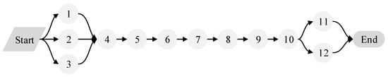
Figure 3.
Construction network plan of Case 1.
The quality weighting coefficients for each construction process and the quality scores for the different construction methods were scored by 10 experienced experts. The detailed construction parameters are shown in Table 2.
Table 2.
Construction parameters of Case 1.
3.1.2. Monte Carlo Simulation
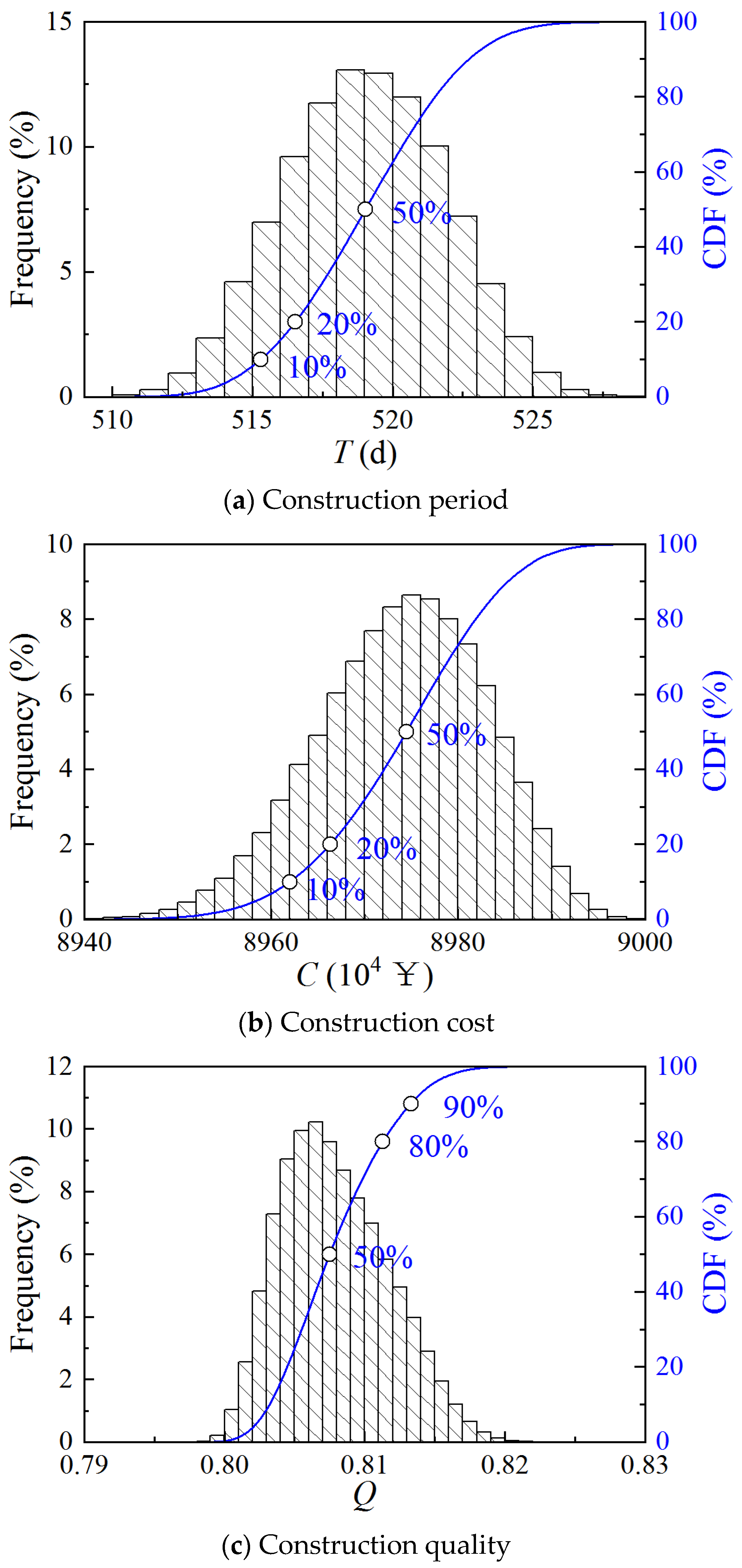
A Monte Carlo simulation was carried out 10,000 times for Case 1, and the cumulative distribution function (CDF) of the three objectives of the construction period, cost, and quality was plotted, as shown in Figure 4.
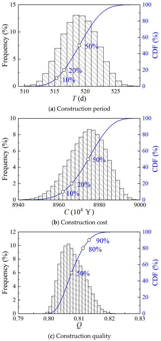
Figure 4.
CDF of construction period, cost, and quality of Case 1.
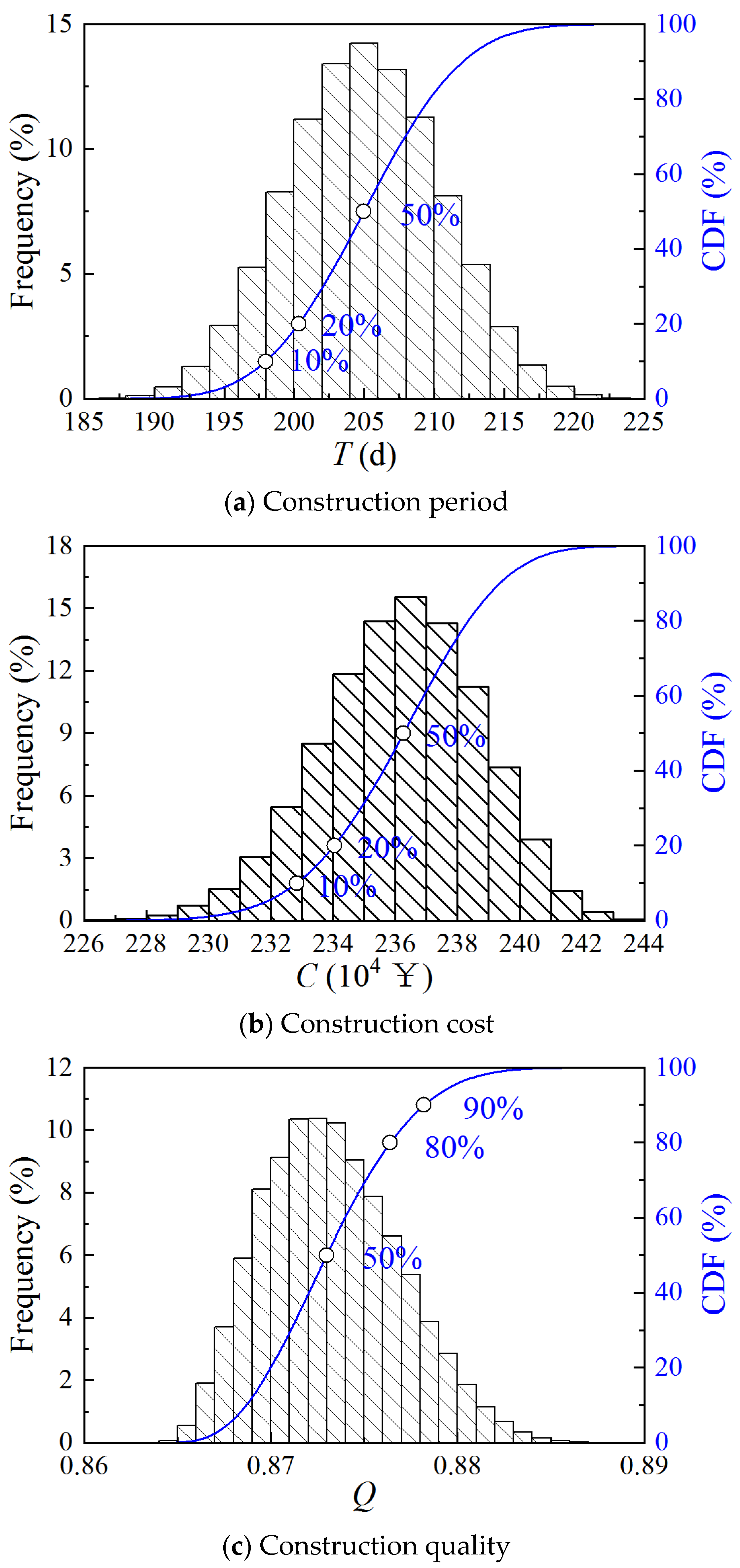
The construction period ranges from 510 to 525 days, the cost ranges from ¥8.94 × 10⁷ to ¥9 × 10⁷, and the quality ranges from 0.80 to 0.82. Approaching Gaussian distributions can be found for the three objectives. Construction period and cost should be as low as possible, and quality should be as high as possible. From a probabilistic point of view, the 50%, 20%, and 10% quartiles for construction period and cost, as well as the 50%, 80%, and 90% quartiles for quality, are informative and reflect the percentage of the current scheme’s objectives that is exceeded.
3.2. Case 2
3.2.1. Construction Parameters
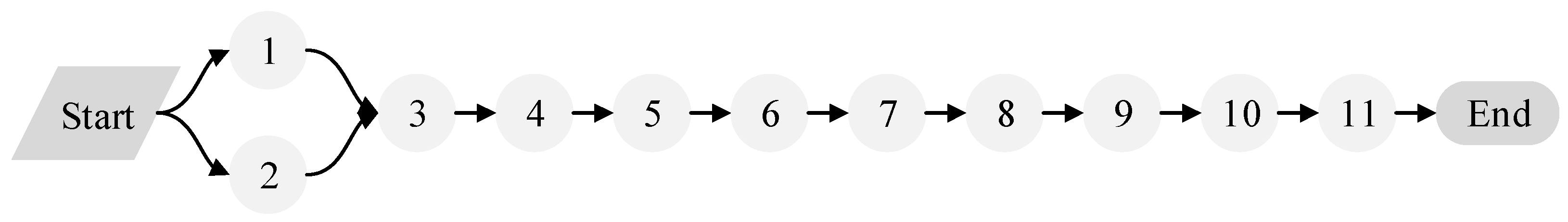
Table 3 displays the construction process of a subway project [25]. It contains a total of 11 processes, and the detailed construction network plan is shown in Figure 5. The subway tunnel project is located in the silty soil layer, coarse and medium sand layer, and pebble layer; the interval span is large; and the construction period is long. The tunnel is tunneled by a mud–water shield machine and is passed through by a two-lane operation. The construction of the tunnel’s left-lane cut-through is taken as a research object.
Table 3.
Content of construction process of Case 2.
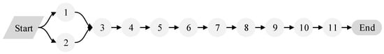
Figure 5.
Construction network plan of Case 2.
The quality scores and weighting coefficients for each construction process and scheme were scored by the project manager, project general engineer, construction technical leader, quality inspection unit leader, superintendent engineer, and five experts. Detailed construction parameters are illustrated in Table 4.
Table 4.
Construction parameters of Case 2.
3.2.2. Monte Carlo Simulation
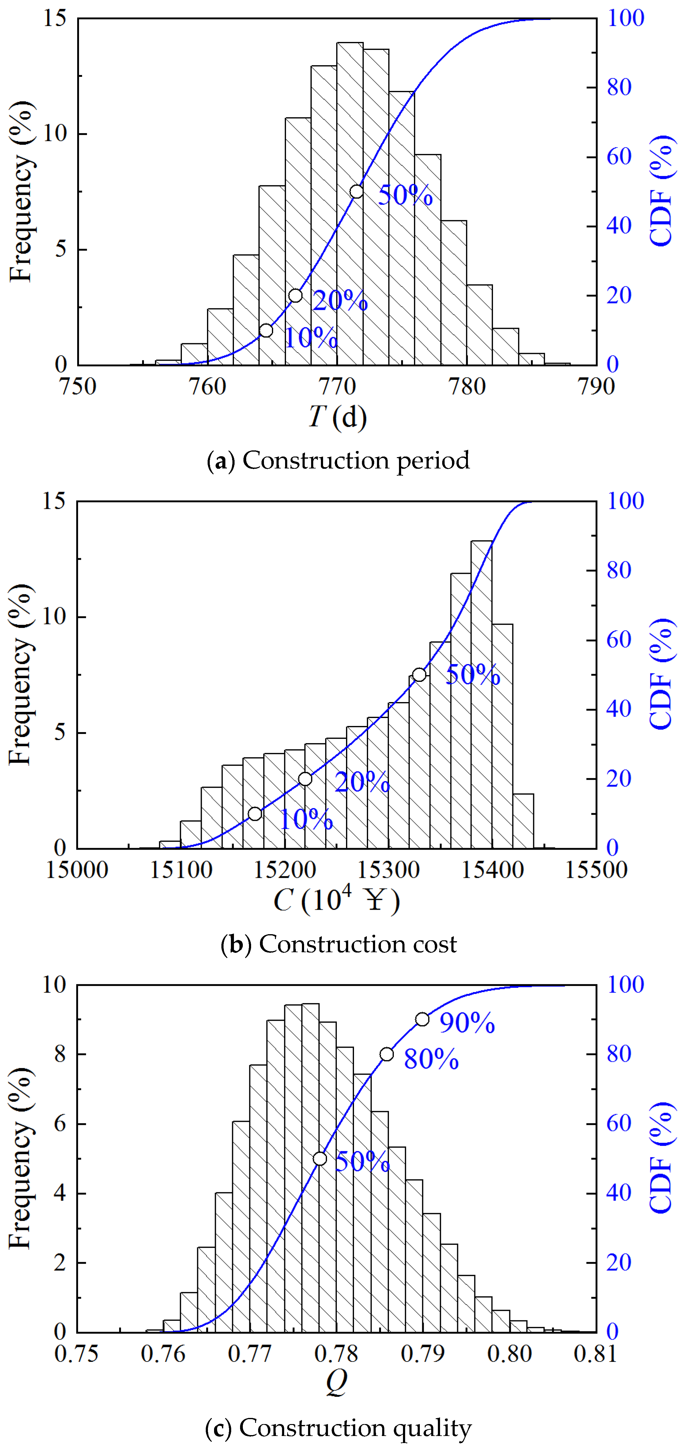
Figure 6 illustrates the CDF obtained from the Monte Carlo simulation for Case 2 for the three objectives of schedule, cost, and quality. The key quartile of the three objectives can be obtained.
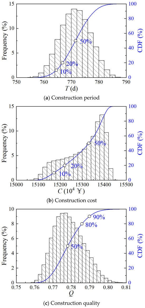
Figure 6.
CDF of construction period, cost, and quality of Case 2.
The construction period ranges from 755 to 790 days, the cost ranges from ¥1.51 × 10⁸ to ¥1.55 × 10⁸, and the quality ranges from 0.76 to 0.80. The overall lower quality scores for Case 2 compared to Case 1 indicate the variability in scoring by different experts, making the use of quartiles of quality scores more informative than absolute values.
3.3. Case 3
3.3.1. Construction Parameters
Table 5 displays the construction process of an airport field road [26]. The airport field road consists of six parts, including a runway, parallel taxiway, fast taxiway, anti-blowout apron, aircraft apron and paddock road, etc. The construction of the airport field road includes five major processes, including construction preparation, earthwork construction, subgrade construction, surface construction, and project completion. The construction network plan of Case 2 is displayed in Figure 7.
Table 5.
Content of construction process of Case 3.
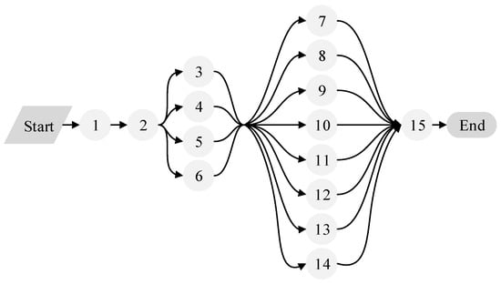
Figure 7.
Construction network plan of Case 3.
The quality scores and detailed construction parameters are shown in Table 6. In this case, it is assumed that each construction process has the same quality weighting factor.
Table 6.
Construction parameters of Case 3.
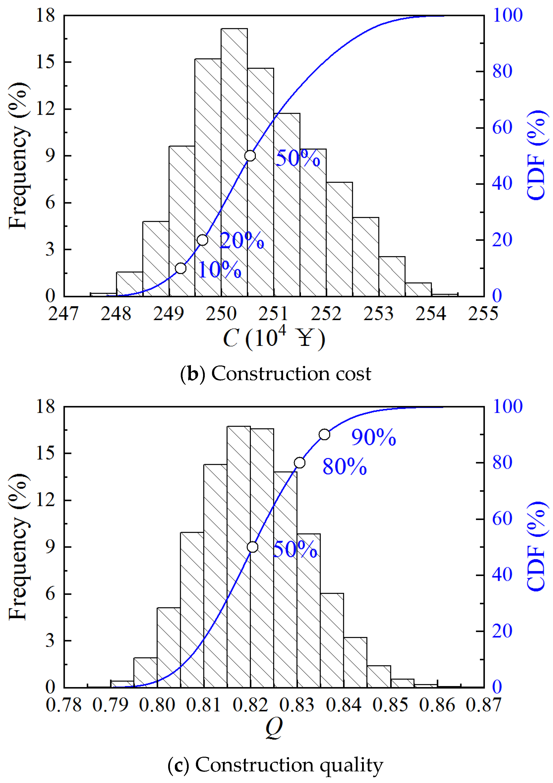
3.3.2. Monte Carlo Simulation
The CDF of the construction period, cost, and quality are obtained by Monte Carlo simulation, as shown in Figure 8. The construction period ranges from 260 to 285 days, the cost ranges from ¥2.47 × 10⁶ to ¥2.55 × 10⁶, and the quality ranges from 0.79 to 0.86. Compared to Case 1 and Case 2, Case 3 has a greater dispersion of quality scores.
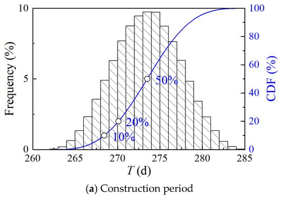
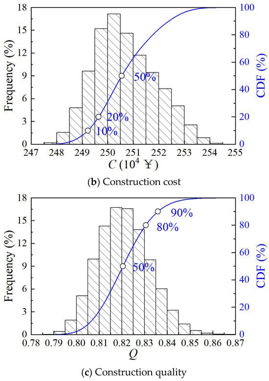
Figure 8.
CDF of construction period, cost, and quality of Case 3.
3.4. Case 4
3.4.1. Construction Parameters
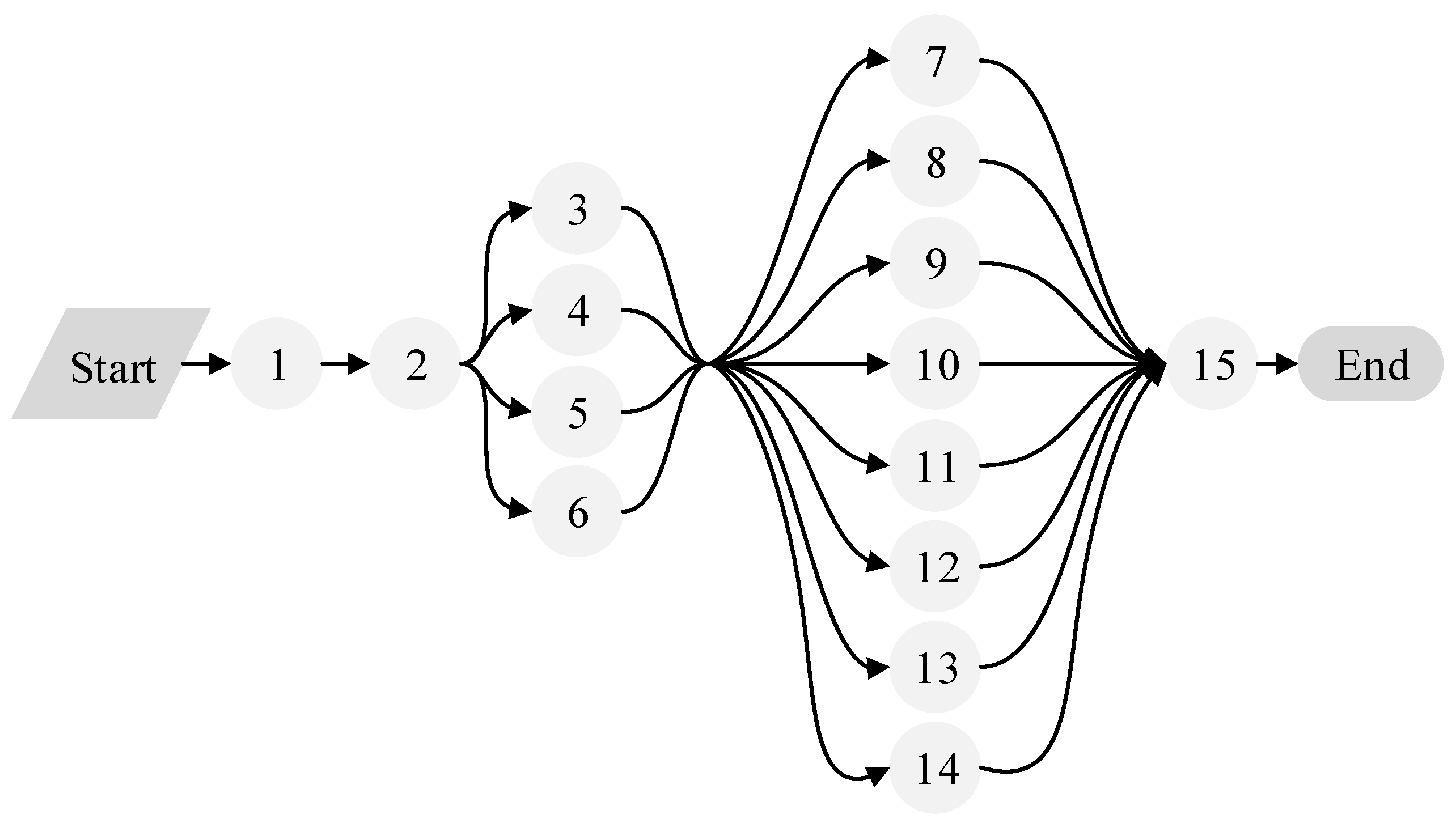
Table 7 displays the construction process of a company’s office building [27]. The building is a three-story brick structure, and the construction network plan is shown in Figure 9, consisting of 19 construction processes. The quality scores and weighting coefficients are offered by 10 experienced program managers. Detailed construction parameters are shown in Table 8.
Table 7.
Content of construction process of Case 4.
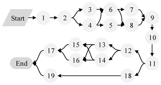
Figure 9.
Construction network plan of Case 4.
Table 8.
Construction parameters of Case 4.
3.4.2. Monte Carlo Simulation
Figure 10 shows the CDF of the construction period, cost, and quality provided by the Monte Carlo simulation. The construction period ranges from 190 to 220 days, the cost ranges from ¥2.27 × 10⁶ to ¥2.43 × 10⁶, and the quality ranges from 0.86 to 0.89. The quality score of Case 4 is much higher than the three cases mentioned above.
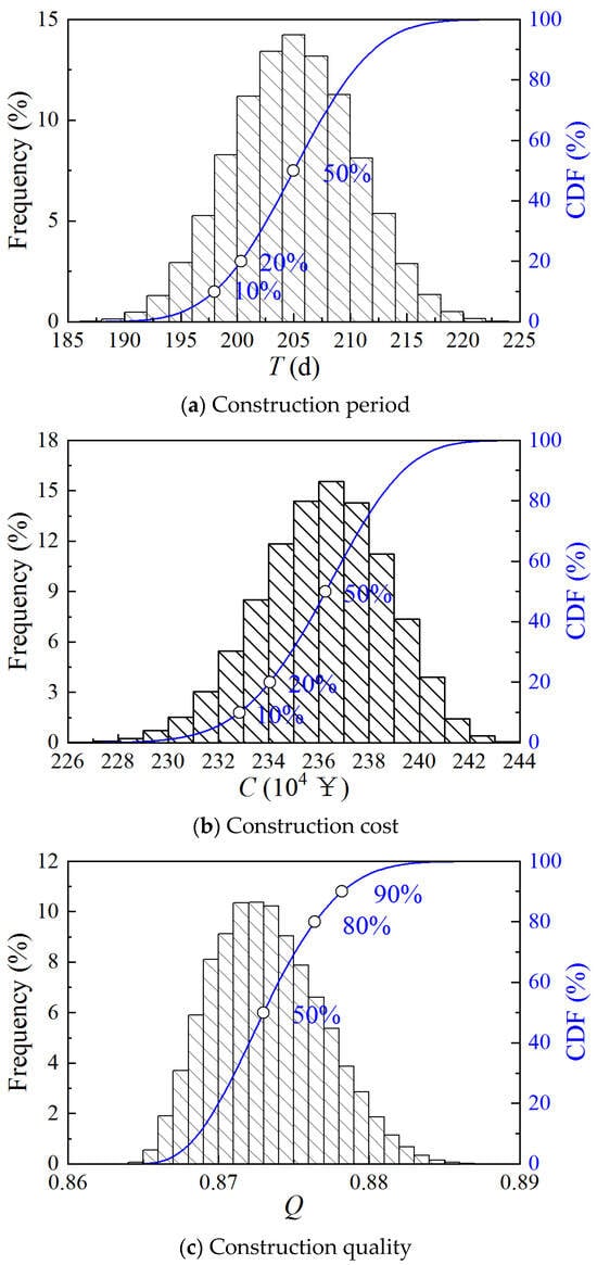
Figure 10.
CDF of construction period, cost, and quality of Case 4.
3.5. Scheme Settings
Through the investigation of the construction project planning phase for the construction period, cost, and quality requirements, six optimization targets were identified to adapt to the demands of various decision-makers, as shown in Table 9. The first three schemes aim to make the third objective as good as possible while constraining the two objectives. Constraints are determined based on Monte Carlo simulation results, e.g., the solution is required to be better than 90% of the feasible solutions in terms of cost and quality while ensuring that the construction period is as short as possible.
Table 9.
Optimization target of construction schemes.
The main parameters of the proposed hybrid approach are set as follows: population size of 200, binary length of 6, cross rate of 0.9, minimum and maximum rate of 0.05 and 0.2, respectively, iteration step of 200, particle size of 100, iteration of 50 for PSO, and initial and final inertial factor of 0.4 and 0.9, respectively. It is important to note that we assume that once the optimized construction plan is finalized, workers will strictly follow the plan, and there is no risk associated with ethics.
4. Results and Discussion
4.1. Case 1
4.1.1. Scheme 1
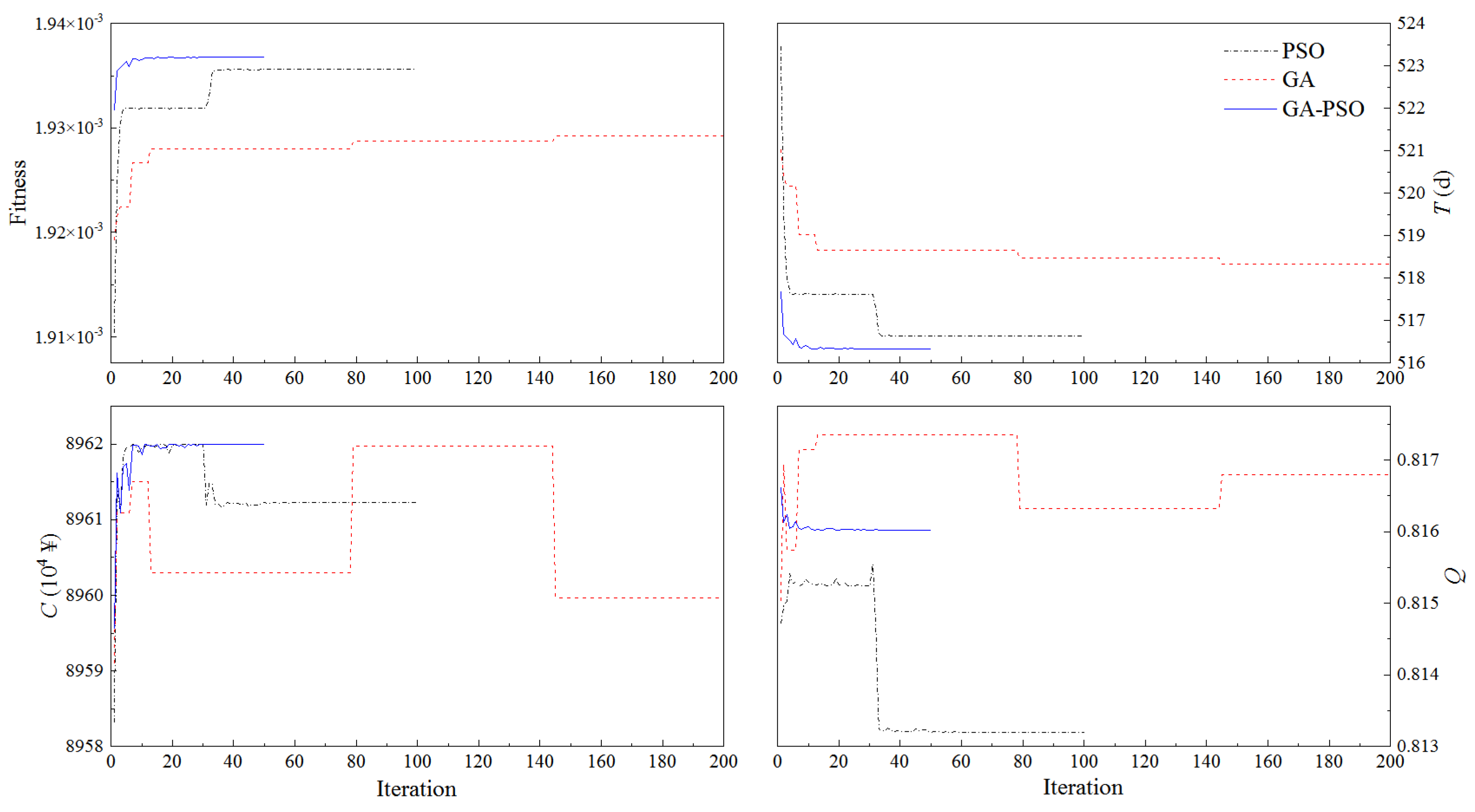
This scheme aims to minimize the construction period under the constraints of cost and quality. The upper limit of construction cost and lower limit of quality are ¥8.962 × 10⁷ and 0.8132, respectively. The iteration process for Scheme 1 of Case 1 can be found in Figure 11, where the fitness denotes the reciprocal of T. It can be found that GA convergence requires the most iterative steps, close to 150, and GA-PSO the shortest, about 20 steps. Furthermore, GA-PSO can provide a better solution than GA and PSO.
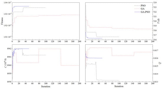
Figure 11.
Iteration process for Scheme 1 of Case 1.
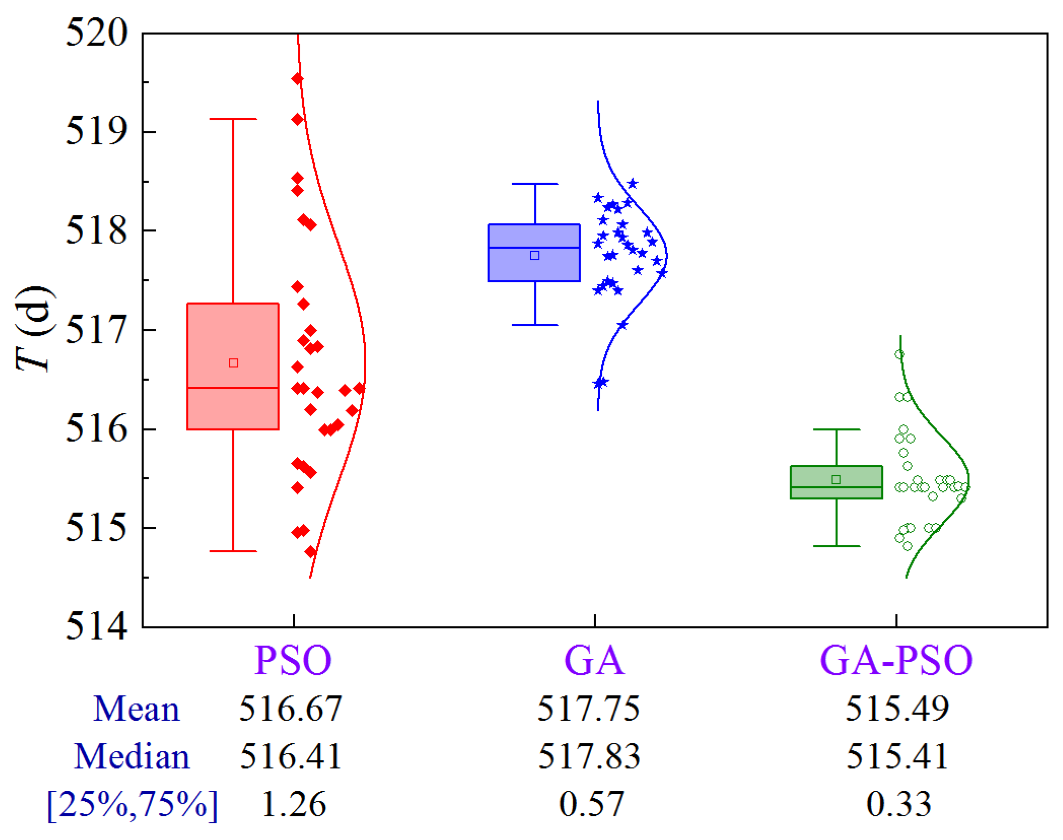
Due to the stochastic nature of the optimization results of GA-based or PSO-based algorithms, uncertainty analysis is required to compare them statistically. Figure 12 shows the uncertainty analysis for Scheme 1 of Case 1 based on 30 replications, where 25% and 75% denote the quartiles and [25%, 75%] denotes the interval between the 25% quartile and the 75% quartile.
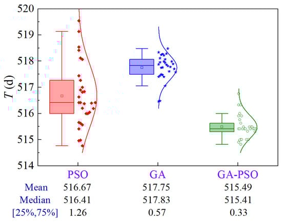
Figure 12.
Uncertainty analysis for Scheme 1 of Case 1.
The results show that PSO has the largest solution volatility, GA is second, and GA-PSO is the most stable. From the optimization performance, GA-PSO > PSO > GA. To quantitatively compare the optimization effects of the three algorithms, three metrics, the mean, median, and interval between 25% quartile and 75% quartile (denoted as volatility), are selected for comprehensive analysis. Compared to PSO and GA, the GA-PSO algorithm reduces the mean and median construction period by 1.18 and 2.26 days, and 1 and 2.42 days, respectively, while the volatility is reduced by 73.8% and 42.1%, respectively.
4.1.2. Scheme 2
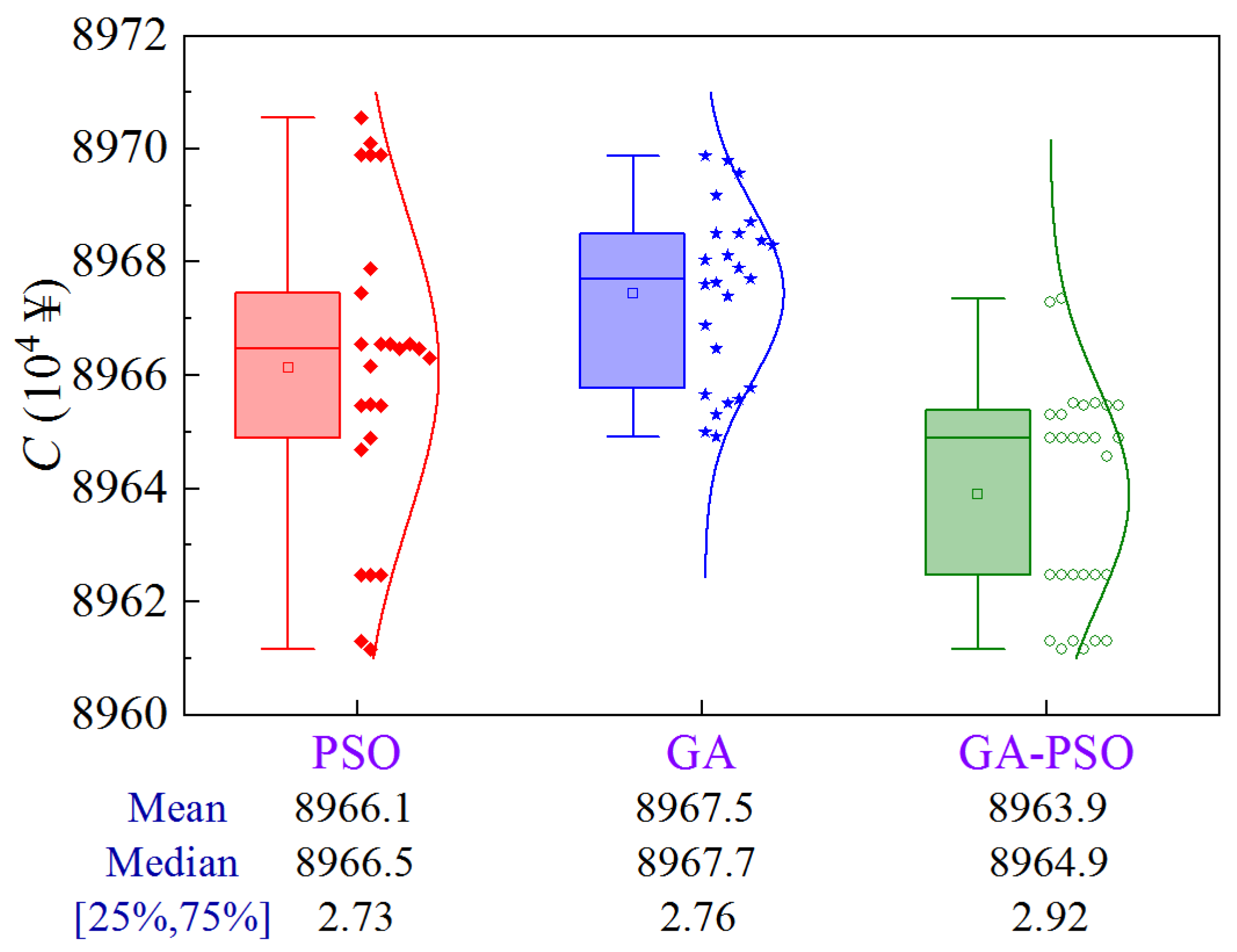
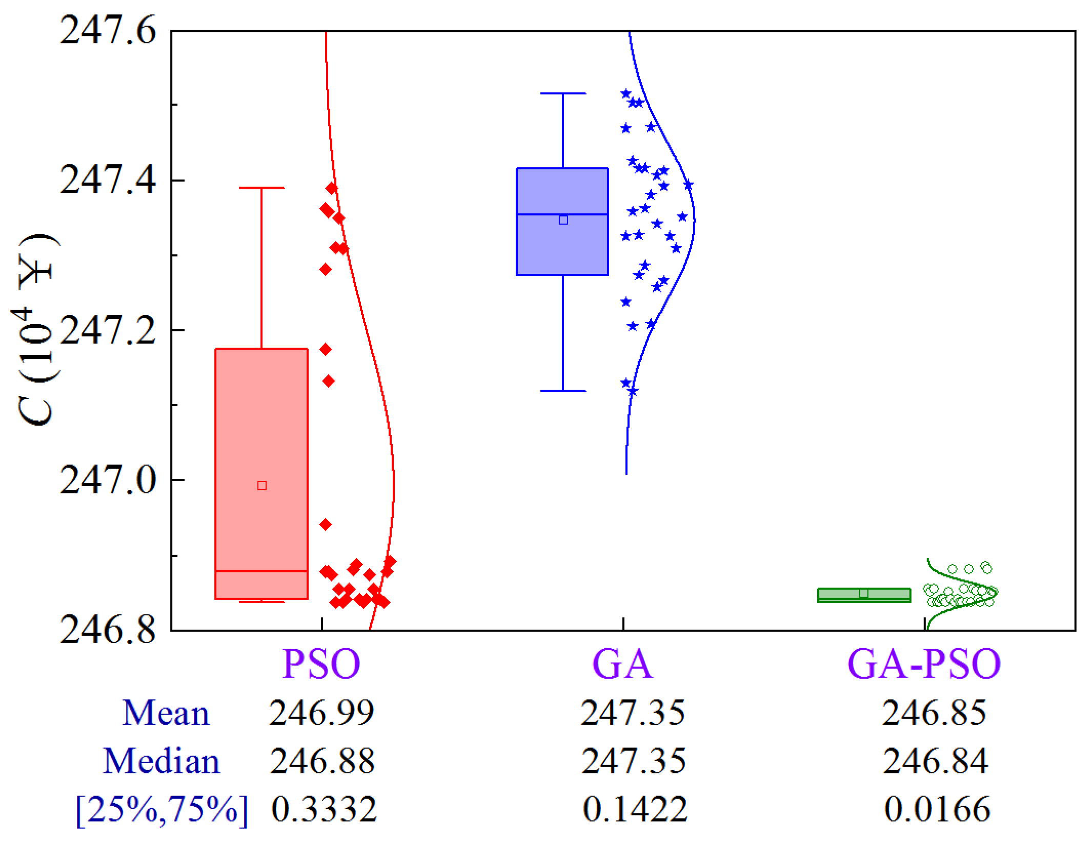
Figure 13 shows the uncertainty analysis for Scheme 2 of Case 1. The upper limit of the construction period and the lower limit of quality are 516.5 d and 0.8113, respectively. Compared to PSO and GA, the GA-PSO algorithm reduces the mean and median construction cost by ¥22,000 and ¥36,000, and ¥16,000 and ¥28,000, respectively, while the volatility is comparable.

Figure 13.
Uncertainty analysis for Scheme 2 of Case 1.
4.1.3. Scheme 3
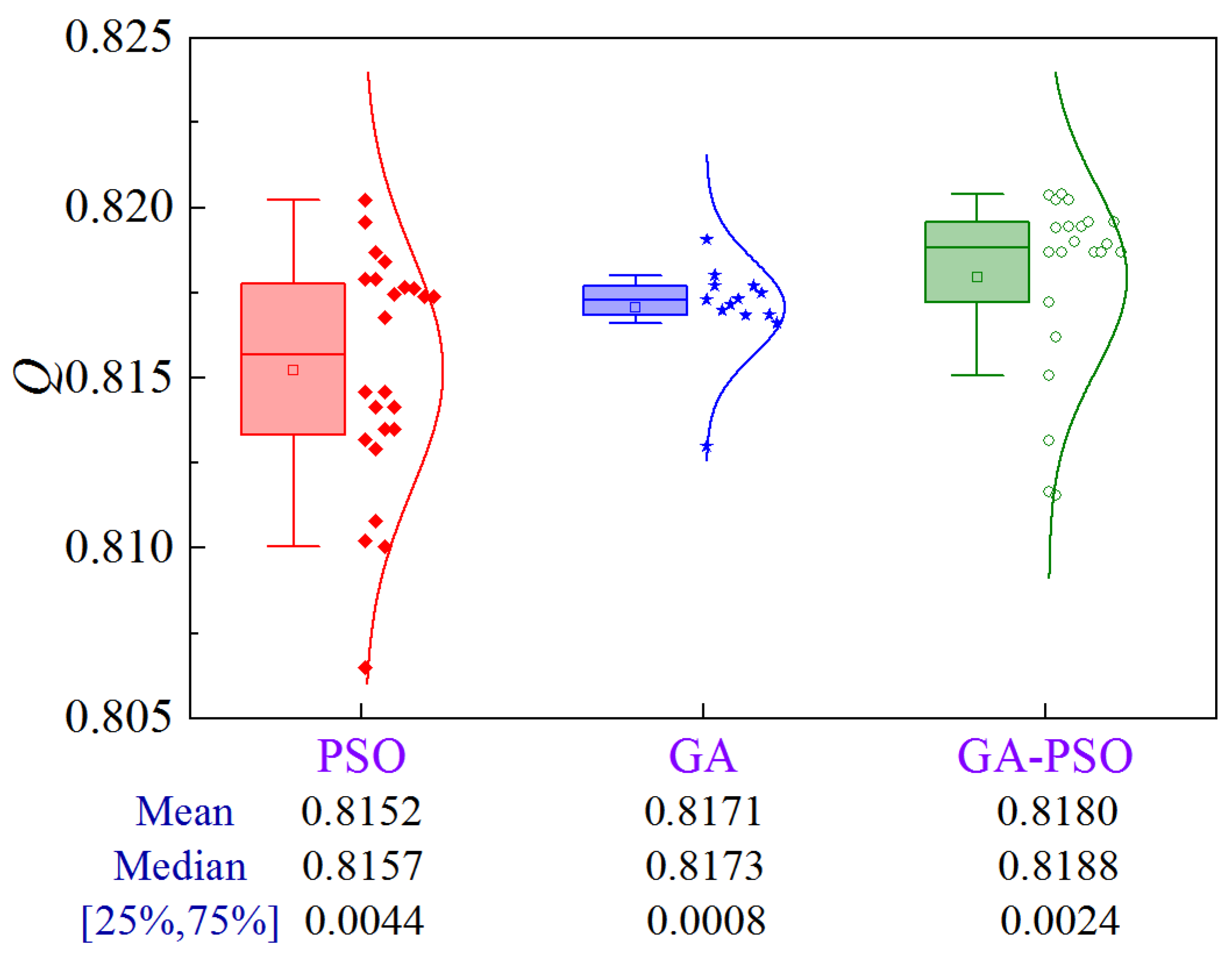
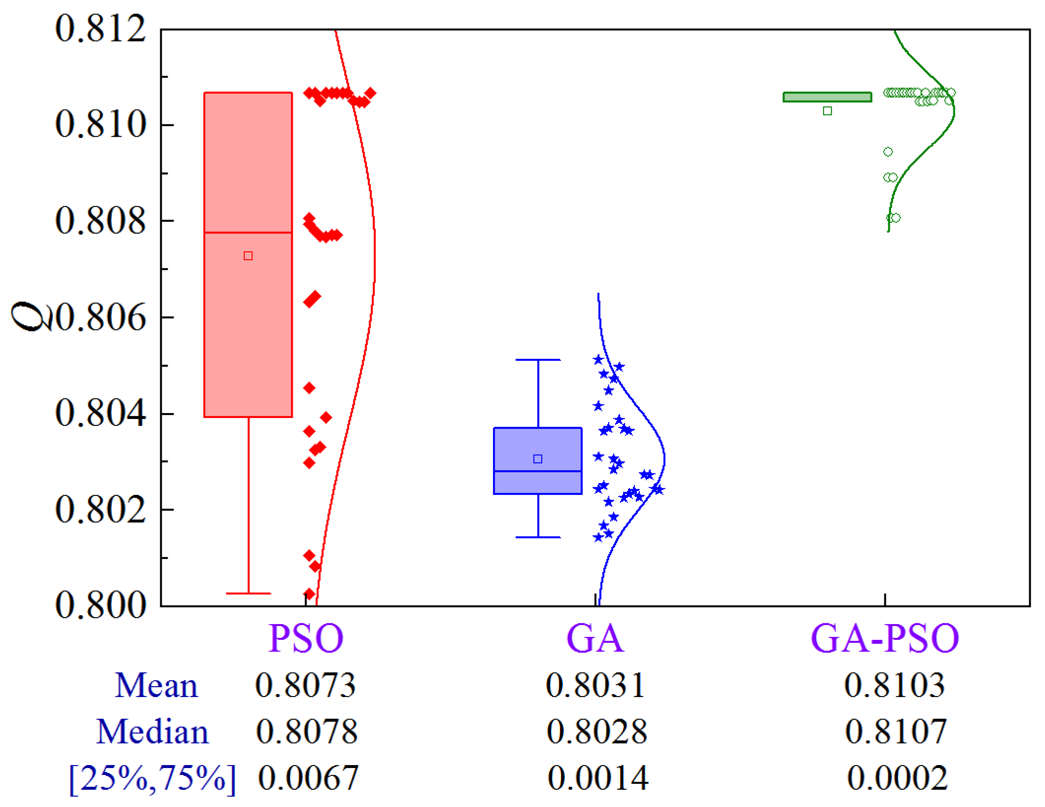
Figure 14 illustrates the uncertainty analysis for Scheme 3 of Case 1. The upper limit of construction period and cost are 516.5 d and ¥8.966 × 10⁷, respectively. The GA-PSO algorithm can provide the best quality in terms of mean and median values. Moreover, the volatility can be reduced by 45.4% compared to PSO.
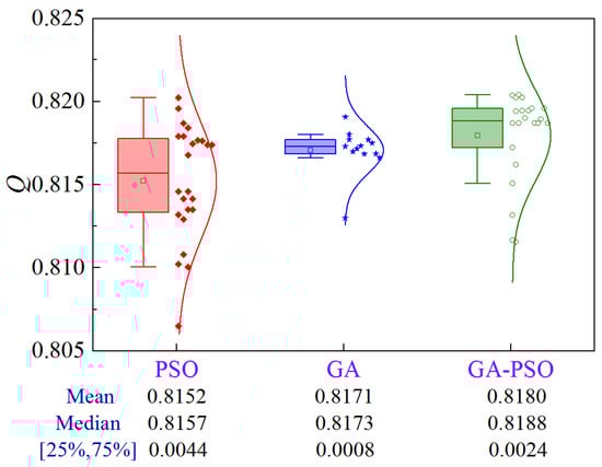
Figure 14.
Uncertainty analysis for Scheme 3 of Case 1.
4.1.4. Scheme 4
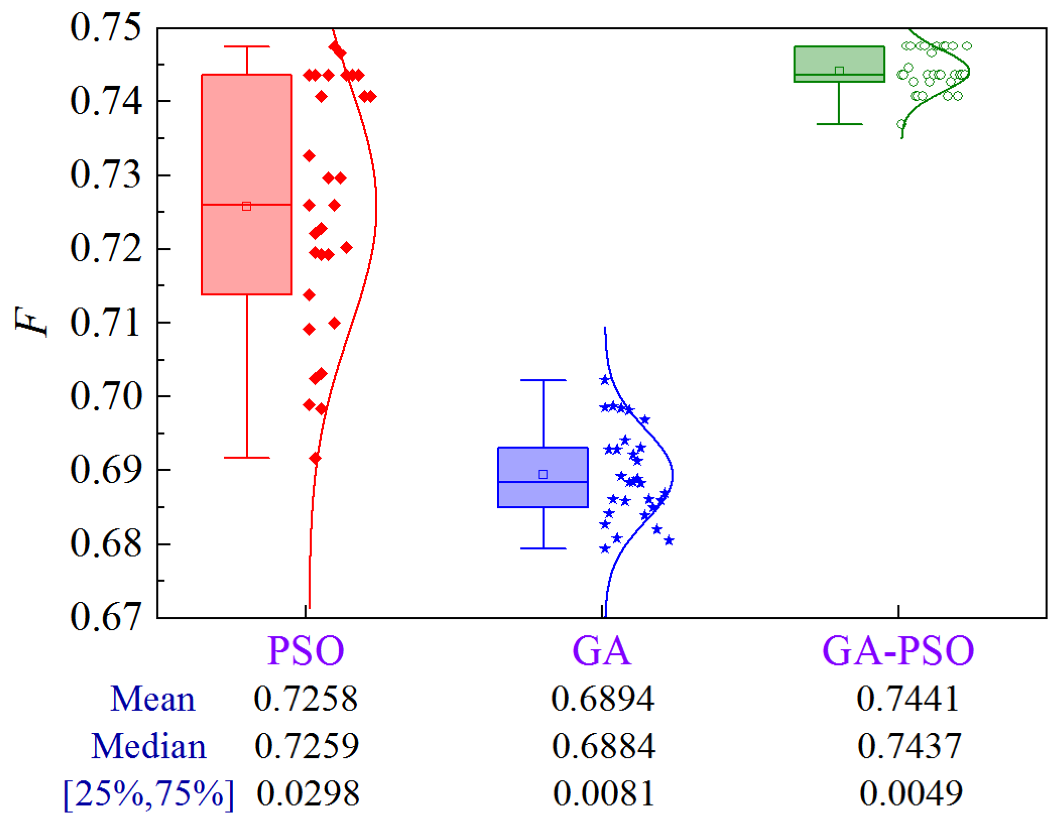
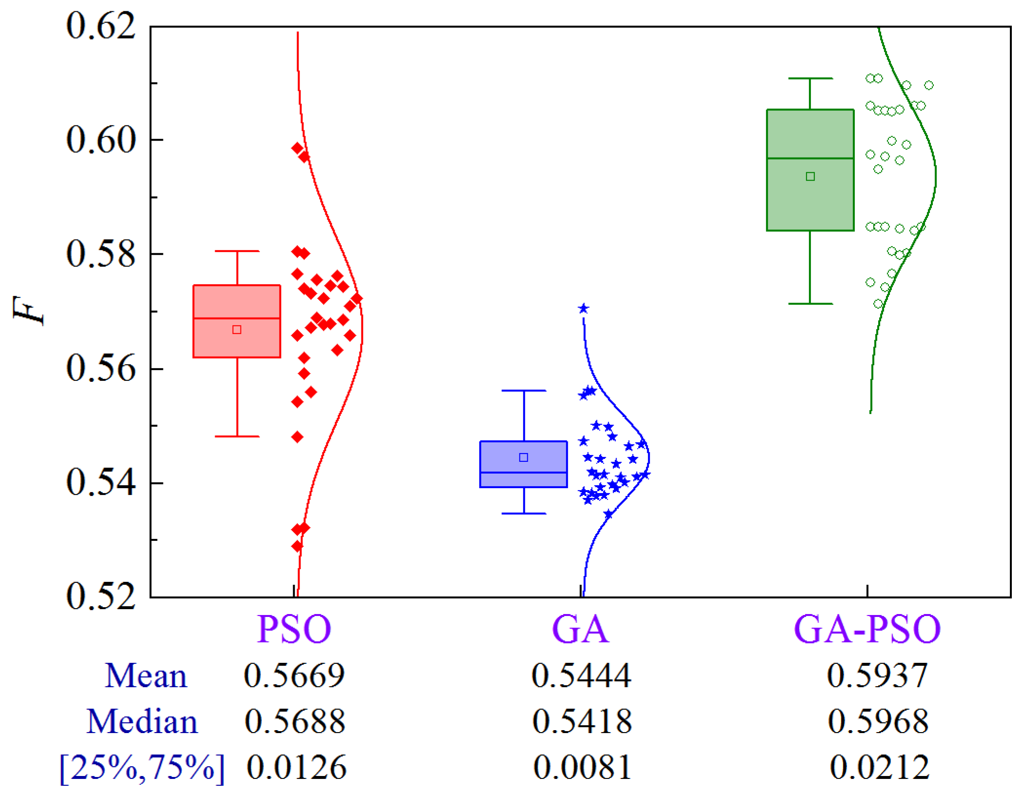
This scheme aims to find the optimal solution by combining normalized construction period, cost, and quality into a composite index through weighting. Figure 15 illustrates the uncertainty analysis for Scheme 4 of Case 1. Compared to PSO and GA, the GA-PSO algorithm enhances the mean and median by 3.4% and 5.3%, and 2.9% and 5.6%, respectively, while decreasing the volatility by approximately 100%.
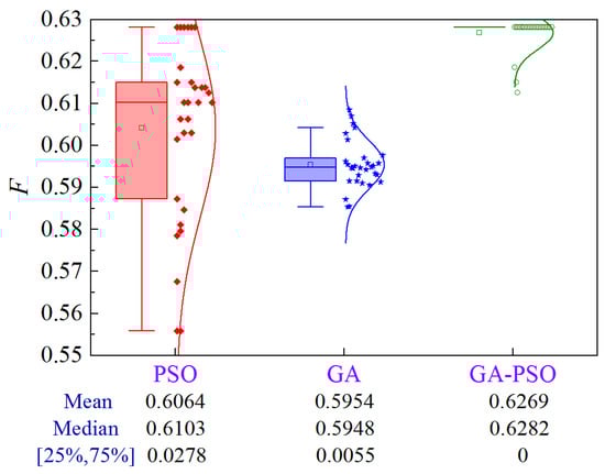
Figure 15.
Uncertainty analysis for Scheme 4 of Case 1.
4.1.5. Scheme 5
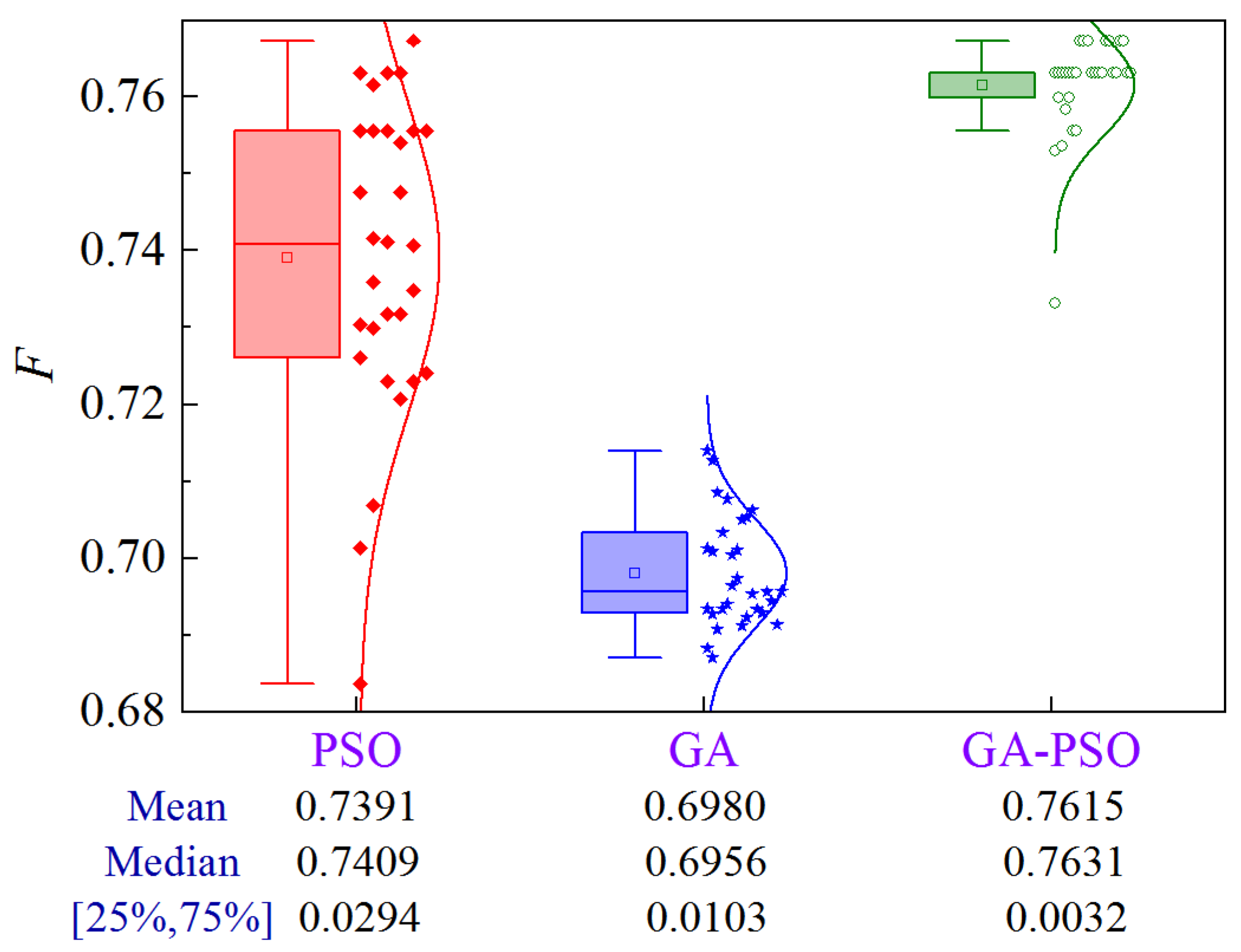
The uncertainty analysis for Scheme 5 of Case 1 is shown in Figure 16. Compared to PSO and GA, the GA-PSO algorithm enhances the mean and median by 4.1% and 5.7%, and 3.6% and 5.6%, respectively, while decreasing the volatility by approximately 100%.
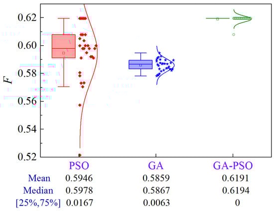
Figure 16.
Uncertainty analysis for Scheme 5 of Case 1.
4.1.6. Scheme 6
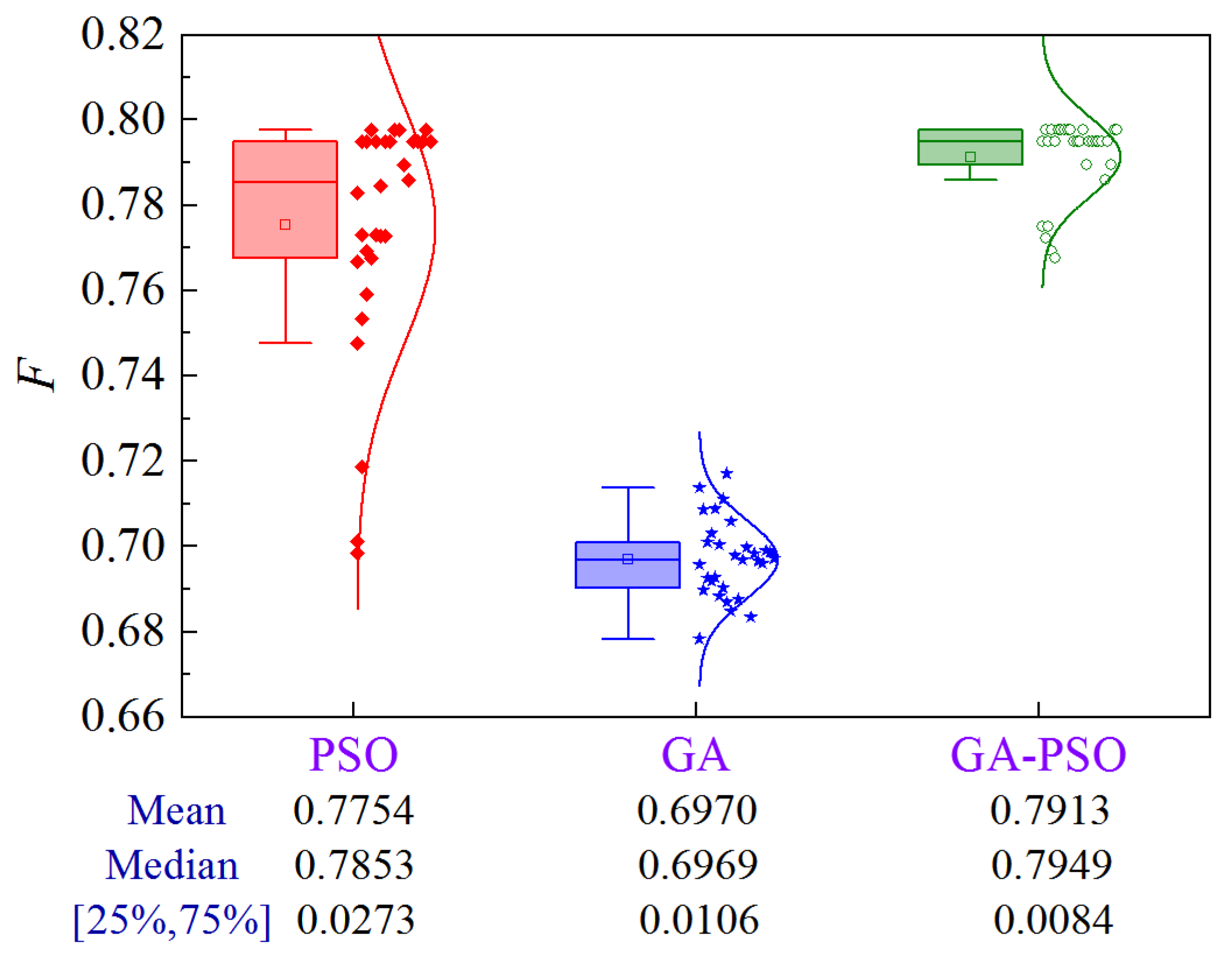
The uncertainty analysis for Scheme 6 of Case 1 is illustrated in Figure 17. Compared to PSO and GA, the GA-PSO algorithm improves the mean and median by 4.8% and 8.6%, and 4.7% and 8.2%, respectively, while eliminating the volatility.
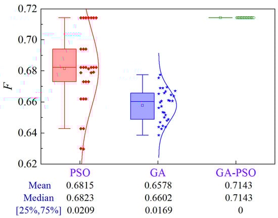
Figure 17.
Uncertainty analysis for Scheme 6 of Case 1.
4.2. Case 2
4.2.1. Scheme 1
Figure 18 shows the uncertainty analysis for Scheme 1 of Case 2. The upper limit of construction cost and lower limit of quality are ¥1.517 × 10⁸ and 0.7899, respectively. Compared to PSO and GA, the GA-PSO algorithm reduces the mean and median construction period by 1.71 and 3.69 days, and 1.71 and 4.03 days, respectively, while the volatility is reduced by 68.2% and 39.8%, respectively.
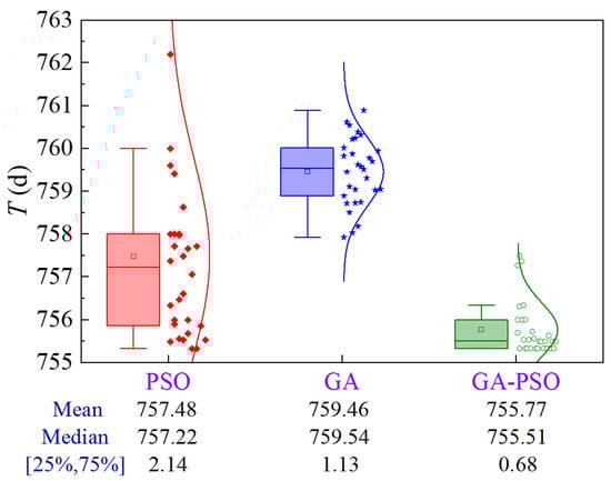
Figure 18.
Uncertainty analysis for Scheme 1 of Case 2.
4.2.2. Scheme 2
Figure 19 shows the uncertainty analysis for Scheme 2 of Case 2. The upper limit of the construction period and the lower limit of quality are 764.5 d and 0.7899, respectively. Compared to PSO and GA, the GA-PSO algorithm reduces the mean and median construction cost by ¥20,000 and ¥166,000, and ¥10,000 and ¥170,000, respectively, while the volatility decreases by 78.1% and 71.8%, respectively.
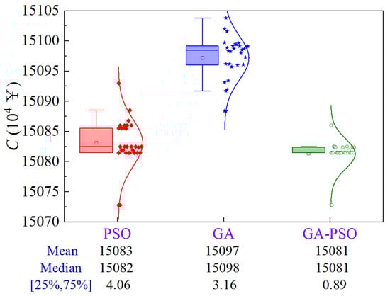
Figure 19.
Uncertainty analysis for Scheme 2 of Case 2.
4.2.3. Scheme 3
Figure 20 illustrates the uncertainty analysis for Scheme 3 of Case 2. The upper limit of the construction period and cost are 764.5 d and ¥1.517 × 10⁸, respectively. The GA-PSO algorithm can provide the best quality in terms of mean and median values. In addition, volatility is reduced by 97.0% and 85.7% compared to PSO and GA, respectively.

Figure 20.
Uncertainty analysis for Scheme 3 of Case 2.
4.2.4. Scheme 4
Figure 21 illustrates the uncertainty analysis for Scheme 4 of Case 2. Compared to PSO and GA, the GA-PSO algorithm enhances the mean and median by 1.8% and 5.5%, and 2.2% and 5.9%, respectively, while decreasing the volatility by 85.8% and 66.3%, respectively.
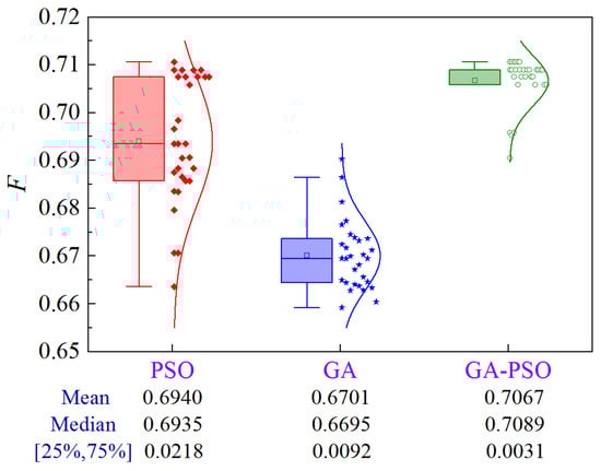
Figure 21.
Uncertainty analysis for Scheme 4 of Case 2.
4.2.5. Scheme 5
Figure 22 illustrates the uncertainty analysis for Scheme 5 of Case 2. Compared to PSO and GA, the GA-PSO algorithm enhances the mean and median by 2.1% and 4.7%, and 2.0% and 5.0%, respectively, while decreasing the volatility by 77.8% and 30.9%, respectively.
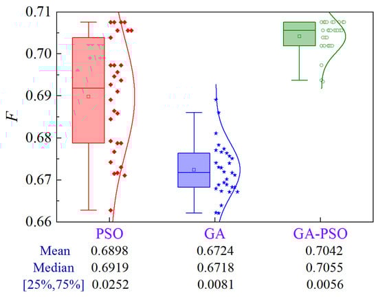
Figure 22.
Uncertainty analysis for Scheme 5 of Case 2.
4.2.6. Scheme 6
The uncertainty analysis for Scheme 6 of Case 2 is illustrated in Figure 23. Compared to PSO and GA, the GA-PSO algorithm improves the mean and median by 2.4% and 7.8%, and 1.7% and 7.9%, respectively, while decreasing the volatility by 95.6% and 88.0%, respectively.
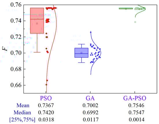
Figure 23.
Uncertainty analysis for Scheme 6 of Case 2.
4.3. Case 3
4.3.1. Scheme 1
Figure 24 shows the uncertainty analysis for Scheme 1 of Case 3. The upper limit of construction cost and lower limit of quality are ¥2.492 × 10⁶ and 0.8359, respectively. Compared to PSO and GA, the GA-PSO algorithm reduces the mean and median construction period by 0.44 and 1.64 days, and 0 and 1.79 days, respectively, while the volatility is reduced by approximately 100%.
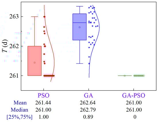
Figure 24.
Uncertainty analysis for Scheme 1 of Case 3.
4.3.2. Scheme 2
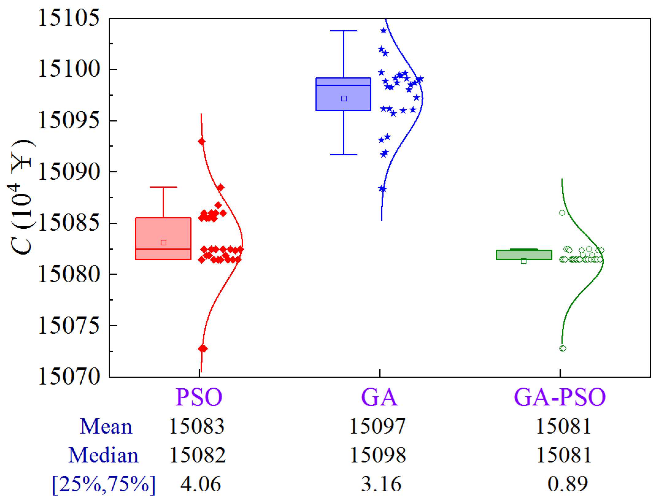
Figure 25 shows the uncertainty analysis for Scheme 2 of Case 3. The upper limit of the construction period and the lower limit of quality are 268.4 d and 0.8359, respectively. Compared to PSO and GA, the GA-PSO algorithm reduces the mean and median construction cost by ¥1400 and ¥5000, and ¥400 and ¥5100, respectively, while the volatility decreases by 95.0% and 88.3%, respectively.
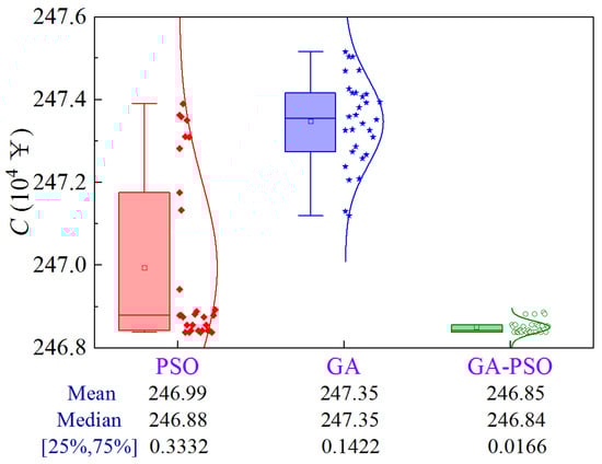
Figure 25.
Uncertainty analysis for Scheme 2 of Case 3.
4.3.3. Scheme 3
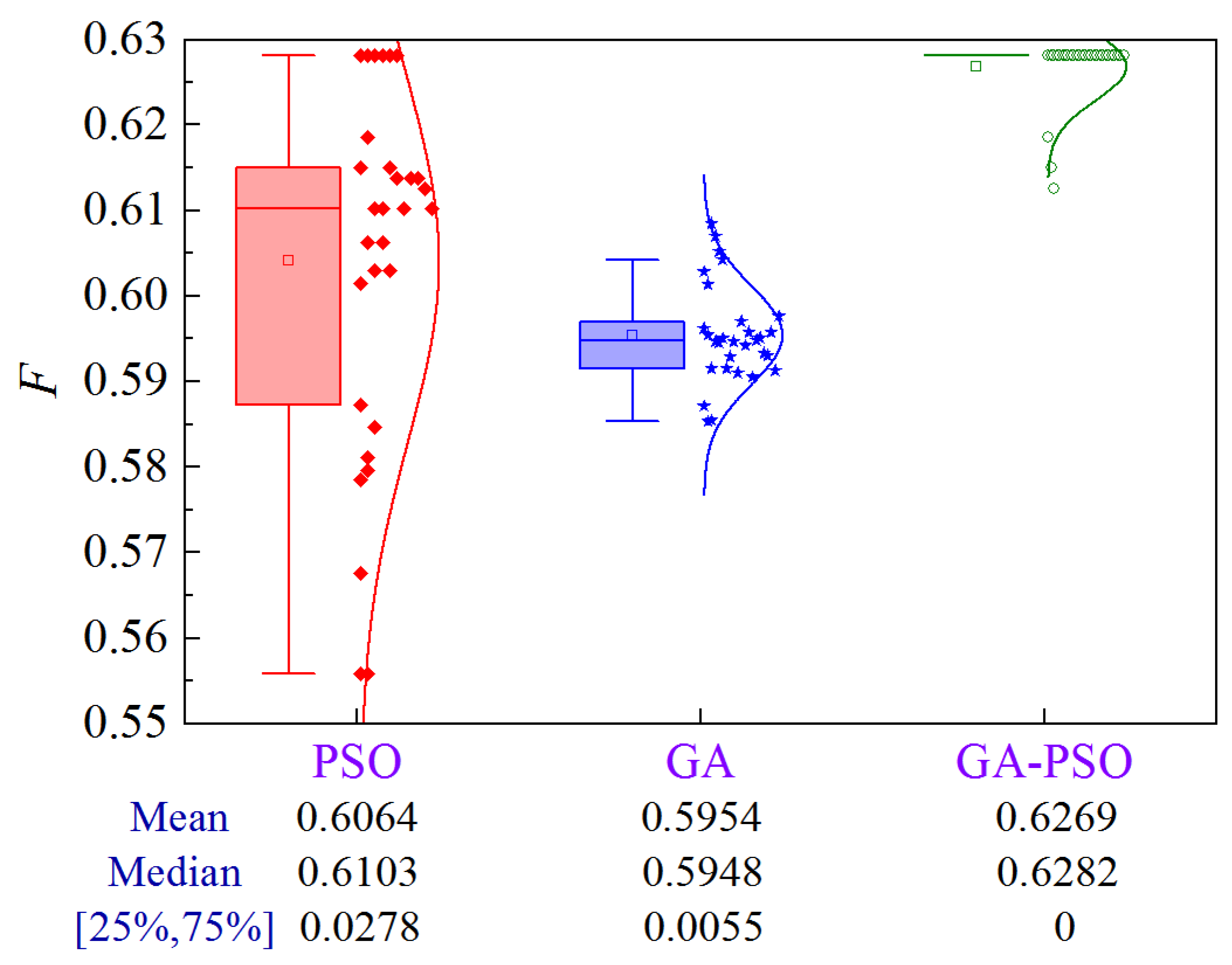
Figure 26 illustrates the uncertainty analysis for Scheme 3 of Case 3. The upper limit of the construction period and cost are 268.4 d and ¥2.492 × 10⁶, respectively. The GA-PSO algorithm can provide the best quality in terms of mean and median values. In addition, volatility is reduced by 55.9% compared to PSO.
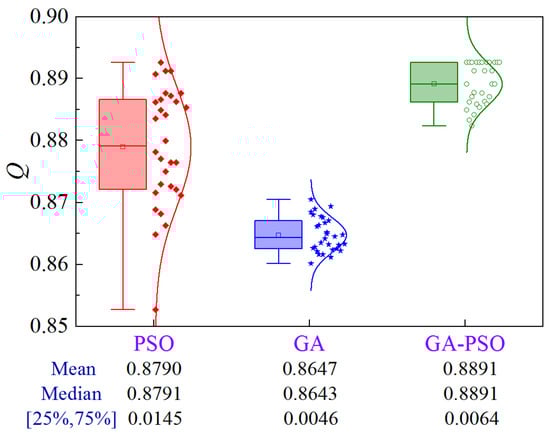
Figure 26.
Uncertainty analysis for Scheme 3 of Case 3.
4.3.4. Scheme 4
Figure 27 illustrates the uncertainty analysis for Scheme 4 of Case 3. Compared to PSO and GA, the GA-PSO algorithm enhances the mean and median by 3.0% and 9.1%, and 3.0% and 9.7%, respectively, while decreasing the volatility by 89.1% and 68.9%, respectively.
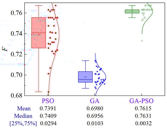
Figure 27.
Uncertainty analysis for Scheme 4 of Case 3.
4.3.5. Scheme 5
Figure 28 illustrates the uncertainty analysis for Scheme 5 of Case 3. Compared to PSO and GA, the GA-PSO algorithm enhances the mean and median by 2.5% and 7.9%, and 2.4% and 8.0%, respectively, while decreasing the volatility by 83.6% and 39.5%, respectively.
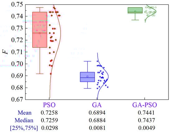
Figure 28.
Uncertainty analysis for Scheme 5 of Case 3.
4.3.6. Scheme 6
The uncertainty analysis for Scheme 6 of Case 3 is illustrated in Figure 29. Compared to PSO and GA, the GA-PSO algorithm improves the mean and median by 2.0% and 13.5%, and 1.2% and 14.1%, respectively, while decreasing the volatility by 69.2% and 20.8%, respectively.
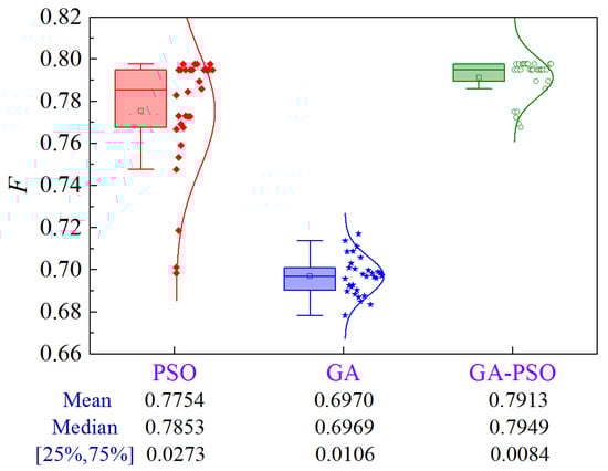
Figure 29.
Uncertainty analysis for Scheme 6 of Case 3.
4.4. Case 4
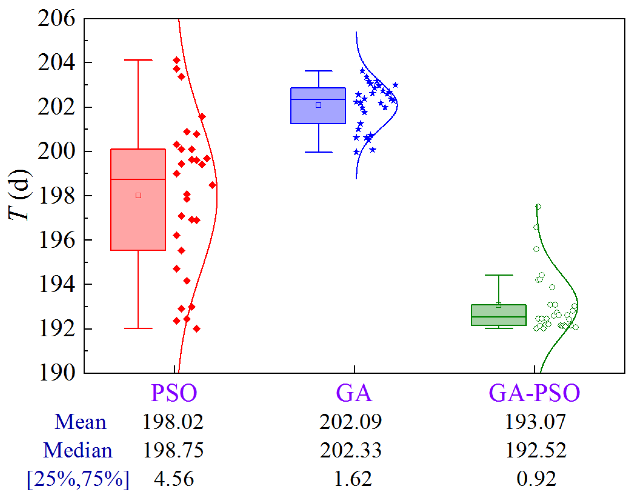
4.4.1. Scheme 1
Figure 30 shows the uncertainty analysis for Scheme 1 of Case 4. The upper limit of construction cost and lower limit of quality are ¥2.328 × 10⁶ and 0.8782, respectively. Compared to PSO and GA, the GA-PSO algorithm reduces the mean and median construction period by 4.95 and 9.02 days, and 6.23 and 9.81 days, respectively, while the volatility is reduced by 79.8% and 43.2%, respectively.
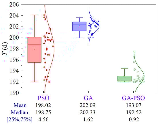
Figure 30.
Uncertainty analysis for Scheme 1 of Case 4.
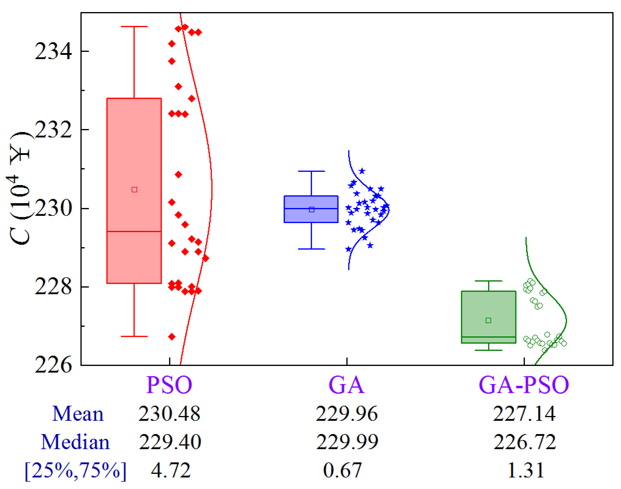
4.4.2. Scheme 2
Figure 31 shows the uncertainty analysis for Scheme 2 of Case 4. The upper limit of the construction period and the lower limit of quality are 198.0 d and 0.8782, respectively. Compared to PSO and GA, the GA-PSO algorithm reduces the mean and median construction cost by ¥33,400 and ¥28,200, and ¥26,800 and ¥32,700, respectively, while the volatility decreases by 72.2% compared to PSO.
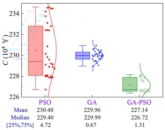
Figure 31.
Uncertainty analysis for Scheme 2 of Case 4.
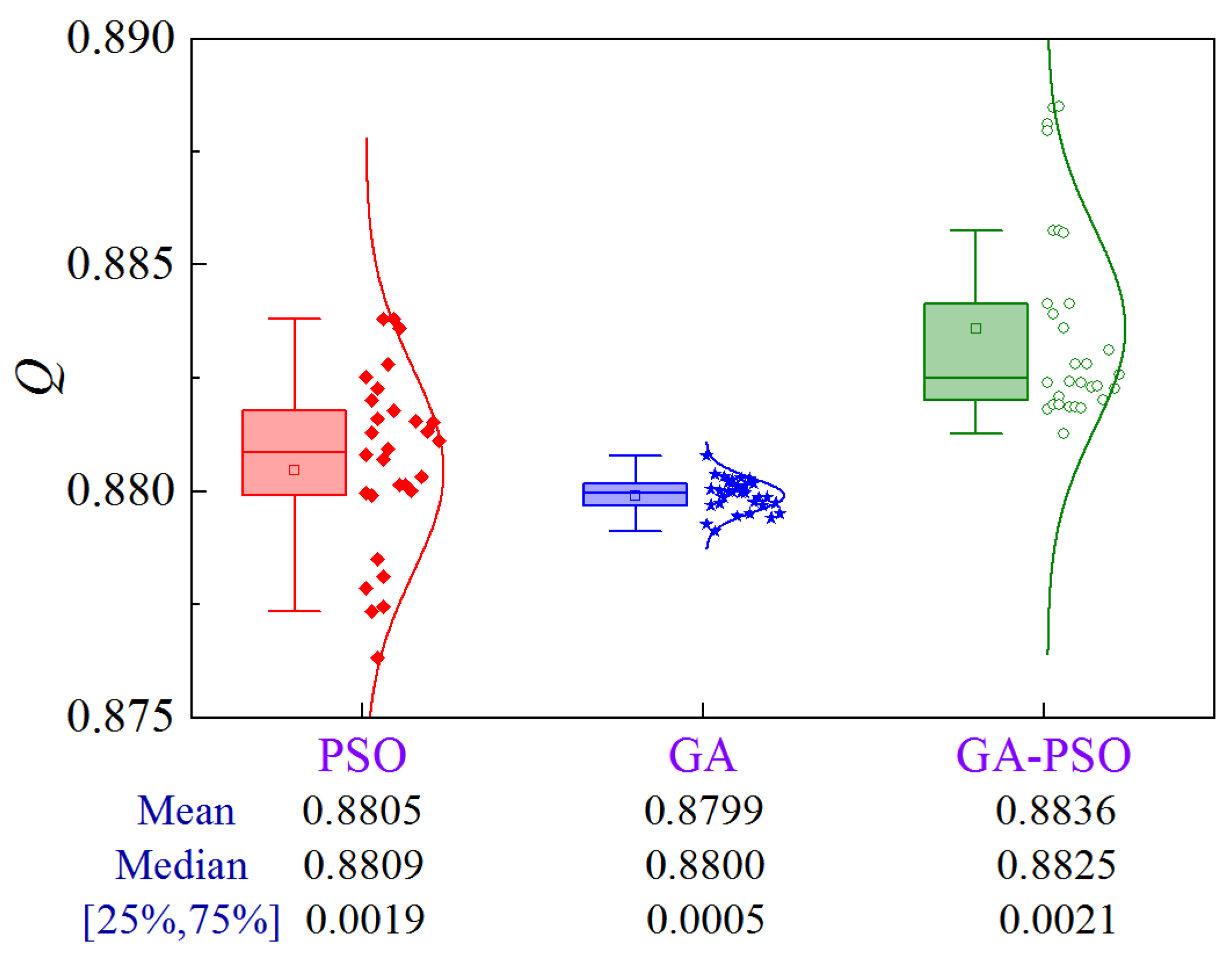
4.4.3. Scheme 3
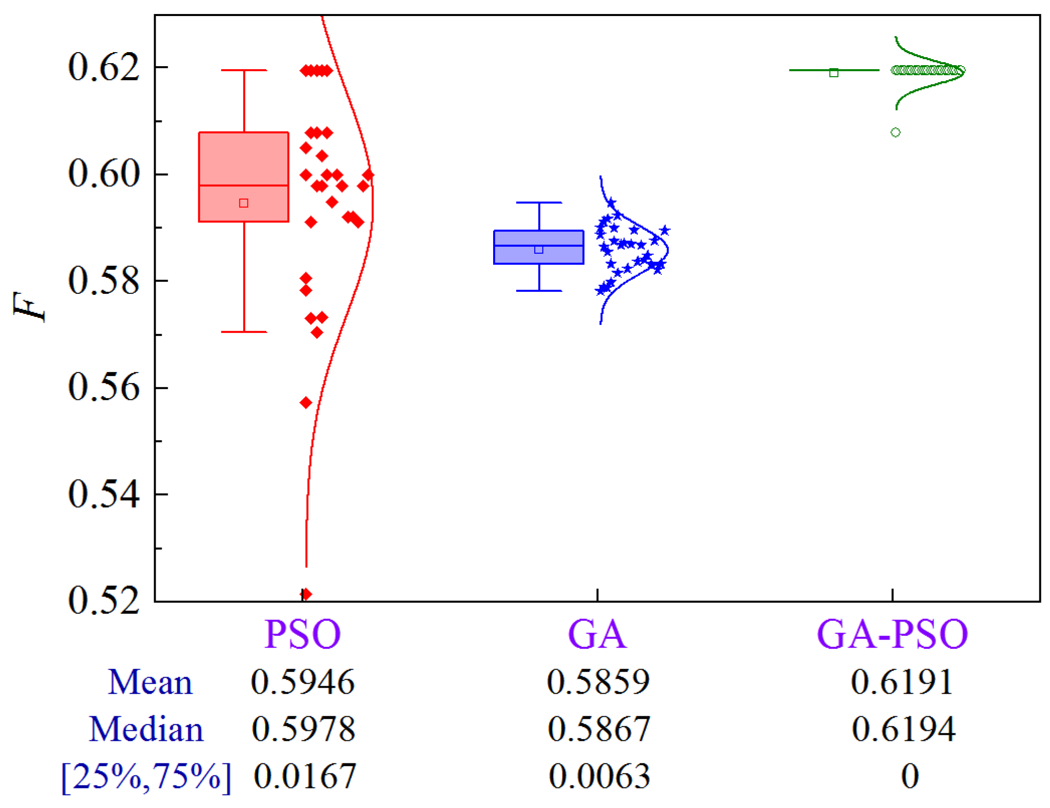
Figure 32 illustrates the uncertainty analysis for Scheme 3 of Case 4. The upper limit of the construction period and cost are 198.0 d and ¥2.328 × 10⁶, respectively. The GA-PSO algorithm can provide the best quality in terms of mean and median values, while the volatility is comparable.
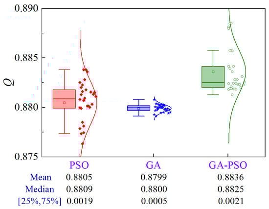
Figure 32.
Uncertainty analysis for Scheme 3 of Case 4.
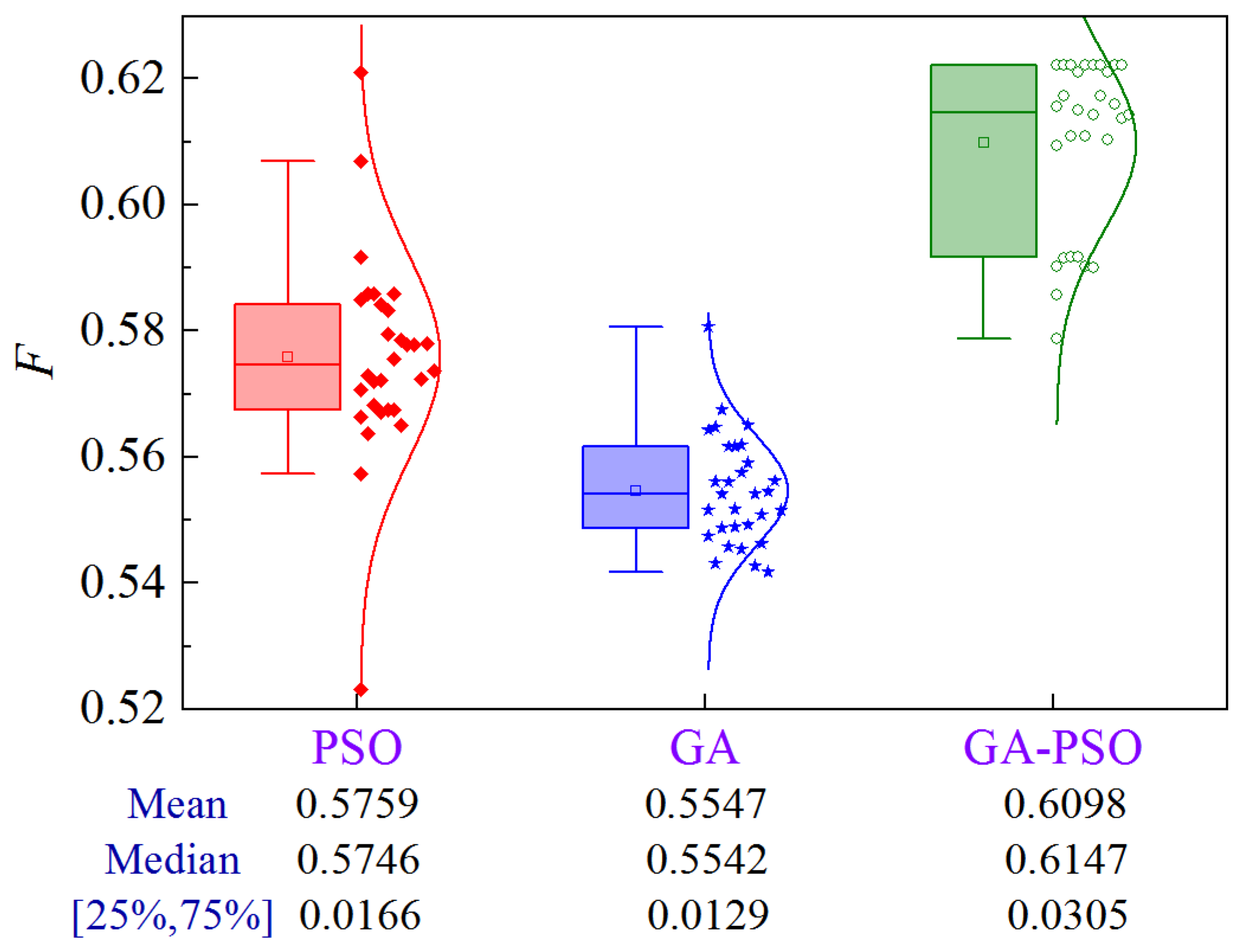
4.4.4. Scheme 4
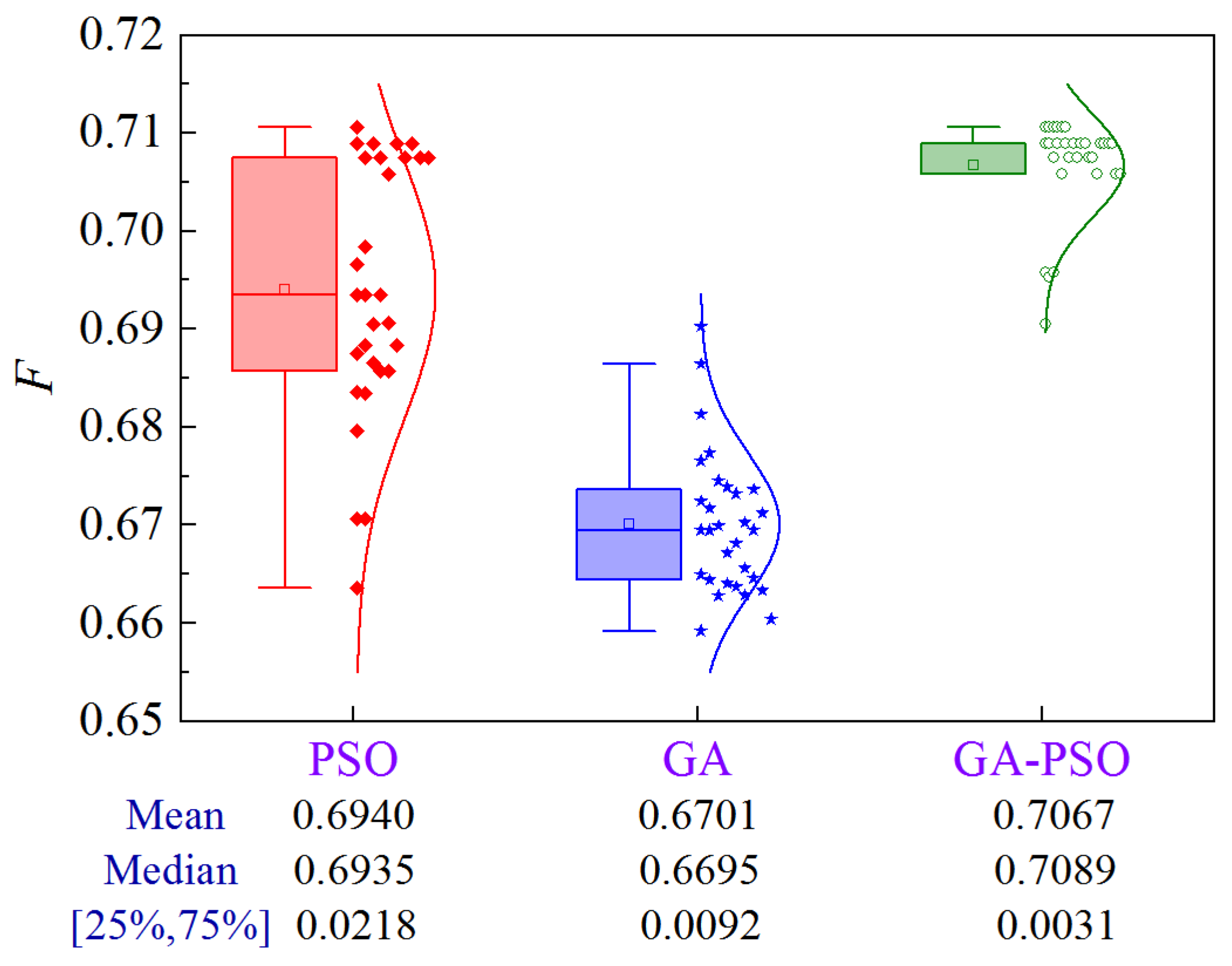
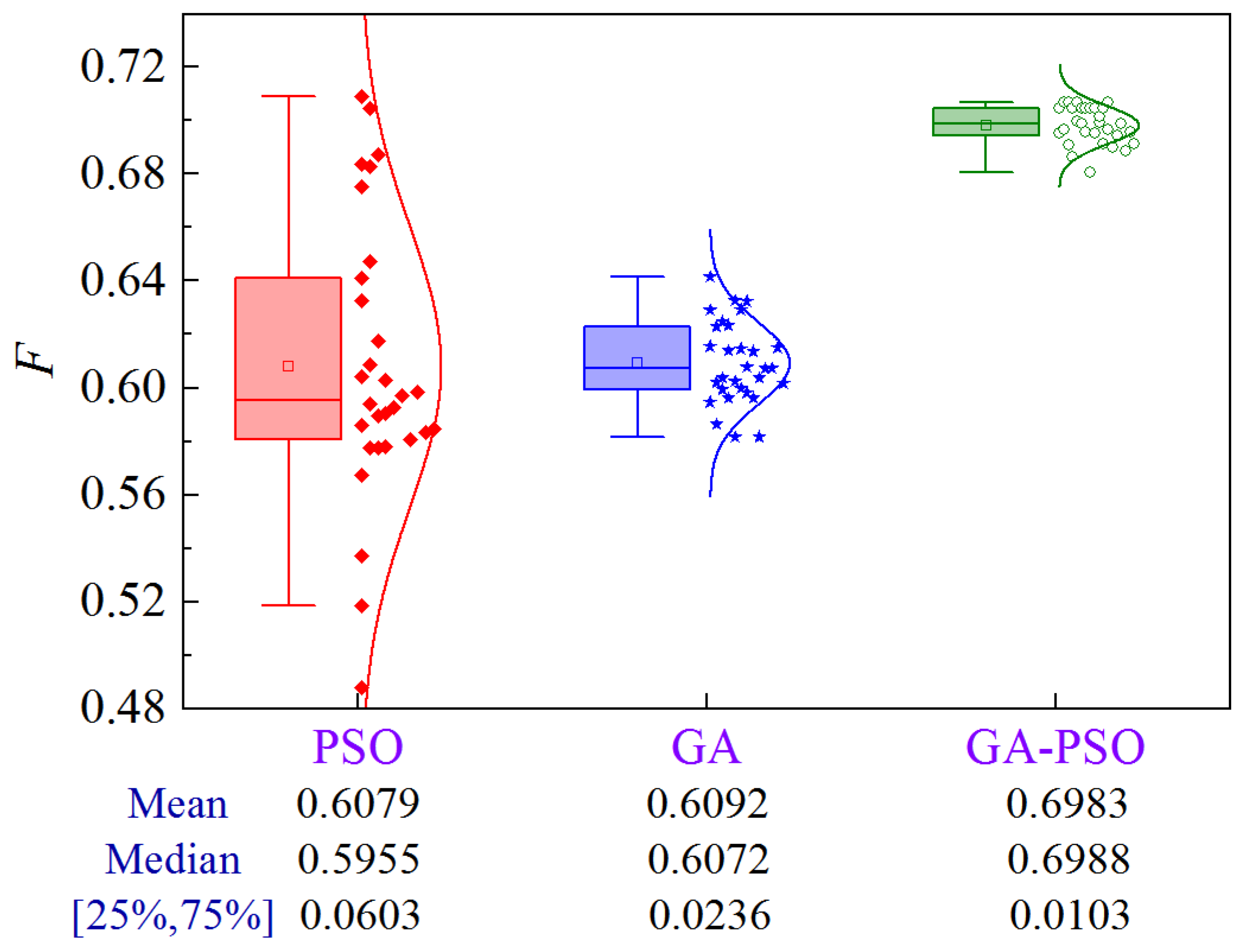
Figure 33 illustrates the uncertainty analysis for Scheme 4 of Case 4. Compared to PSO and GA, the GA-PSO algorithm enhances the mean and median by 5.9% and 9.9%, and 7.0% and 10.9%, respectively.
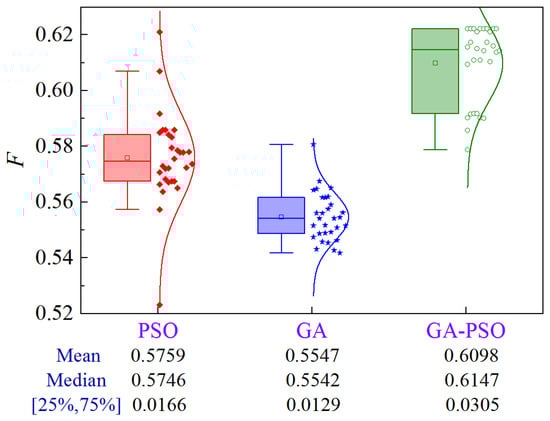
Figure 33.
Uncertainty analysis for Scheme 4 of Case 4.
4.4.5. Scheme 5
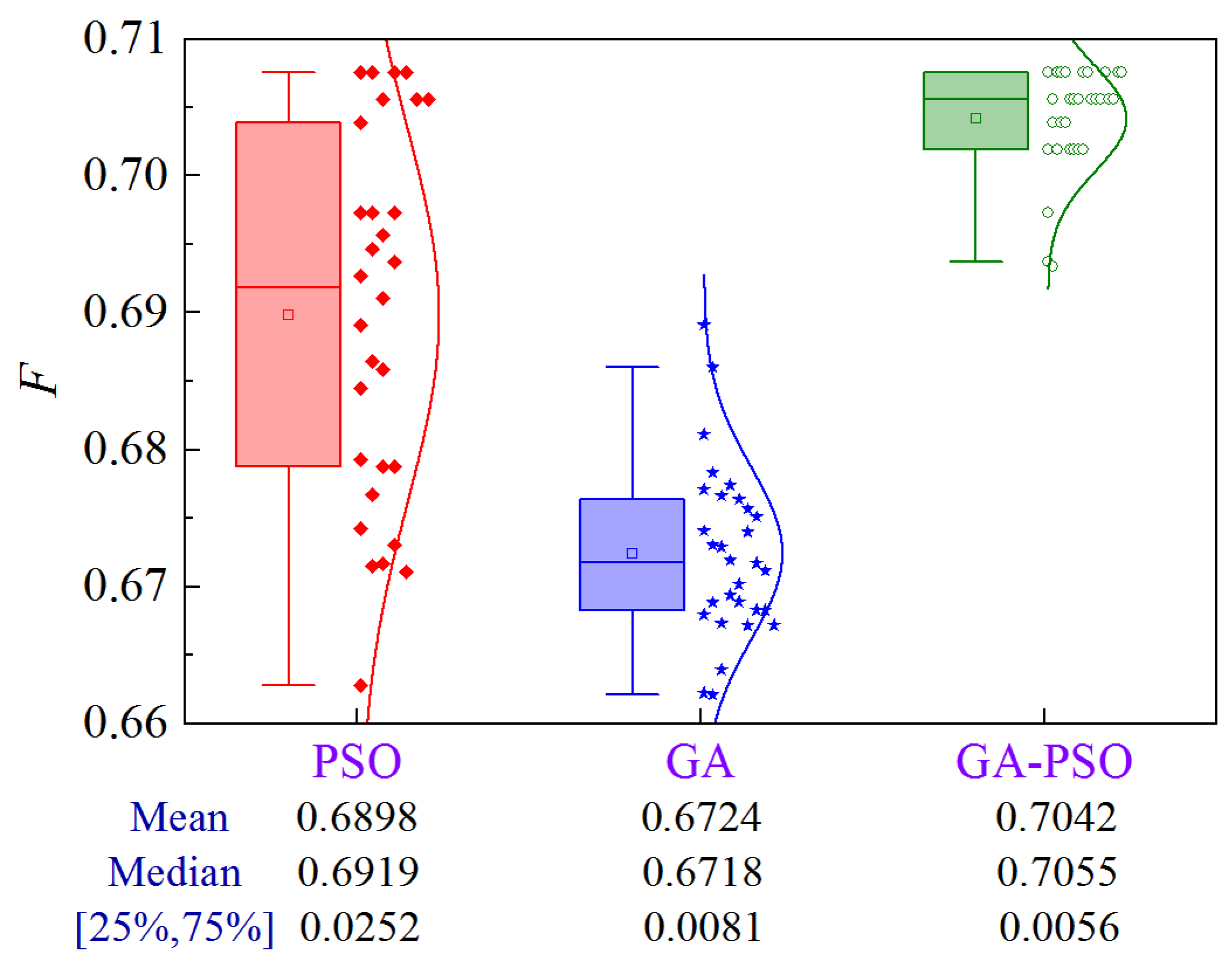
Figure 34 illustrates the uncertainty analysis for Scheme 5 of Case 4. Compared to PSO and GA, the GA-PSO algorithm enhances the mean and median by 4.7% and 9.1%, and 4.9% and 10.2%, respectively.

Figure 34.
Uncertainty analysis for Scheme 5 of Case 4.
4.4.6. Scheme 6
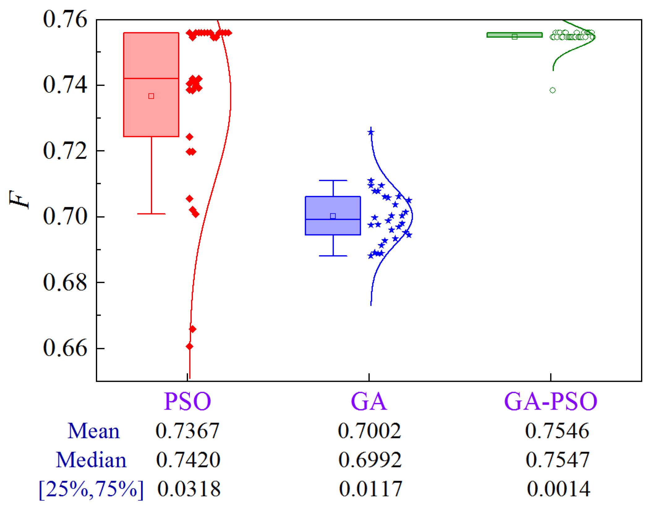
The uncertainty analysis for Scheme 6 of Case 4 is illustrated in Figure 35. Compared to PSO and GA, the GA-PSO algorithm improves the mean and median by 14.9% and 14.6%, and 17.4% and 15.1%, respectively, while decreasing the volatility by 82.9% and 56.4%, respectively.
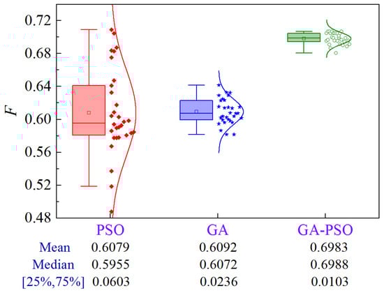
Figure 35.
Uncertainty analysis for Scheme 6 of Case 4.
4.5. Comprehensive Analysis
Table 10 shows the improvements of the proposed GA-PSO compared to PSO and GA for all cases. For the first three schemes, i.e., making the third objective as good as possible while constraining the two objectives, GA-PSO can provide the optimized solution to shorten the construction period by 0.44–4.95 days and 1.64–9.02 days, reduce the cost by ¥1400–33,400 and ¥5000–166,000, and improve the quality by 0.0028–0.0101 and 0.0009–0.0244, respectively, compared with PSO and GA. For the last three objectives, i.e., the three objectives are weighted to form a composite indicator, GA-PSO improves the optimized solution by 4.3% and 8.5% compared to PSO and GA, respectively. Furthermore, GA-PSO can significantly diminish the volatility of optimized solutions. Compared to PSO and GA, GA-PSO reduces volatility by 62.3% and 19.5% for the first three schemes and 66.5% and 55.6% for the last three schemes, respectively. In summary, the proposed hybrid algorithm can reduce volatility by 64.4% and 37.5%, respectively, compared to PSO and GA. The results show that compared to the existing methods, the proposed method provides a superior and more stable solution when performing multi-objective optimization for construction projects. The main reason is that the original GA and PSO can easily fall into the local optimum, while the proposed GA-PSO can break through the low-resolution limitation of the original GA and provide quite good initial particles for the PSO, thus always obtaining the optimization results with better performance.
Table 10.
Improvements of proposed GA-PSO for all cases.
5. Conclusions
A novel hybrid approach combining improved GA and PSO is proposed to optimize construction projects, and various construction projects and optimization targets are studied in-depth. The main findings of this paper can be summarized as follows:
- (1)
- Compared with existing PSO and GA methods, the proposed GA-PSO improves the optimization performance by shortening the construction period by 0.44–9.02 d, reducing the cost by ¥1400–166,000, and enhancing the quality by 0.0009–0.0244 when constraining the two objectives while optimizing the third objective, while improving the performance by 4.3–8.5% when utilizing comprehensive multi-objective optimization targets.
- (2)
- The proposed GA-PSO can reduce the volatility of optimized plans by 19.5–66.5% compared to PSO and GA.
- (3)
- In the comprehensive analysis, the proposed multi-objective hybrid optimization algorithm can improve the optimized construction plan by 4.3–8.5% and, meanwhile, decrease the volatility of the optimized plan by 37.5–64.4%, which can provide a reference for the optimization of construction organization of the construction project.
The main difference in optimization for different projects is the calculation of the fitness function. Although the multi-objective optimization method for construction engineering proposed in this paper is better compared with the existing methods, the provided scheme does not take into account the continuity of the actual construction, such as the duration of the programmed process may be an integer multiple of 1 h, for example, 3 h or 12 h. Therefore, there is a subsequent need to take into full consideration the constraints of the construction process and the feasibility of multi-objective optimization design.
Author Contributions
Writing—original draft preparation, W.H.; formal analysis, Y.Z.; methodology, L.L.; writing—review and editing, P.Z.; validation, J.Q.; resources, B.N. All authors have read and agreed to the published version of the manuscript.
Funding
This research was funded by the National Key R & D Program of China (Grant No. 2022YFB2602204), the National Natural Science Foundation of China (Grant No. 52208479, 52178425), the Jiangxi Provincial Natural Science Foundation (Grant No. 20232BAB204082, 20224BAB214070), and the State Key Laboratory of Performance Monitoring and Protecting of Rail Transit Infrastructure (HJGZ2023205).
Data Availability Statement
The original contributions presented in the study are included in the article, further inquiries can be directed to the corresponding author.
Conflicts of Interest
The authors declare that they have no known competing financial interests or personal relationships that could have appeared to influence the work reported in this paper.
References
- Chen, H.; Wang, J. Multi-objective Optimization for Roadway Maintenance Engineering Based on ev-MOGA. IOP Conf. Ser. Earth Environ. Sci. 2021, 676, 012111. [Google Scholar] [CrossRef]
- Essam, N.; Khodeir, L.; Fathy, F. Approaches for BIM-based multi-objective optimization in construction scheduling. Ain Shams Eng. J. 2023, 14, 102114. [Google Scholar] [CrossRef]
- Wu, K.; García de Soto, B. Spatio-temporal optimization of construction elevator planning in high-rise building projects. Dev. Built Environ. 2024, 17, 100328. [Google Scholar] [CrossRef]
- Li, X.; Zhao, S.; Shen, Y.; Xue, Y.; Li, T.; Zhu, H. Big data-driven TBM tunnel intelligent construction system with automated-compliance-checking (ACC) optimization. Expert Syst. Appl. 2024, 244, 122972. [Google Scholar] [CrossRef]
- Pourgholamali, M.; Labi, S.; Sinha, K.C. Multi-objective optimization in highway pavement maintenance and rehabilitation project selection and scheduling: A state-of-the-art review. J. Road Eng. 2023, 3, 239–251. [Google Scholar] [CrossRef]
- Morin, T.L.; Marsten, R.E. An Algorithm for Nonlinear Knapsack Problems. Manag. Sci. 1976, 22, 1147–1158. [Google Scholar] [CrossRef]
- Ameri, M.; Jarrahi, A.; Haddadi, F.; Mirabimoghaddam, M.H. A Two-Stage Stochastic Model for Maintenance and Rehabilitation Planning of Pavements. Math. Probl. Eng. 2019, 2019, 3971791. [Google Scholar] [CrossRef]
- France-Mensah, J.; Sankaran, B.; O’Brien, W.J. A Bi-Objective Highway Maintenance and Rehabilitation Budget Allocation Approach for Multiple Funding Categories. Constr. Res. Congr. 2018, 2018, 444–454. [Google Scholar]
- Sun, Y.; Hu, M.; Zhou, W.; Xu, W. Multiobjective Optimization for Pavement Network Maintenance and Rehabilitation Programming: A Case Study in Shanghai, China. Math. Probl. Eng. 2020, 2020, 3109156. [Google Scholar] [CrossRef]
- Hu, W.; Yang, Q.; Chen, H.-P.; Guo, K.; Zhou, T.; Liu, M.; Zhang, J.; Yuan, Z. A novel approach for wind farm micro-siting in complex terrain based on an improved genetic algorithm. Energy 2022, 251, 123970. [Google Scholar] [CrossRef]
- Katoch, S.; Chauhan, S.S.; Kumar, V. A review on genetic algorithm: Past, present, and future. Multimed. Tools Appl. 2021, 80, 8091–8126. [Google Scholar] [CrossRef]
- Hu, W.; Yang, Q.; Yuan, Z.; Yang, F. Wind Farm Layout Optimization in Complex Terrain based on CFD and IGA-PSO. Energy 2024, 288, 129745. [Google Scholar] [CrossRef]
- Hu, W.; Yang, Q.; Zhang, J.; Hu, J. Coupled On-Site Measurement/CFD Based Approach for Wind Resource Assessment and Wind Farm Micro-Siting over Complex Terrain. IOP Conf. Ser. Earth Environ. Sci. 2020, 455, 012037. [Google Scholar] [CrossRef]
- Wadea, S.; Bismark, A. Assignments of Pavement Treatment Options: Genetic Algorithms versus Mixed-Integer Programming. J. Transp. Eng. Part B Pavements 2020, 146, 4020008. [Google Scholar]
- Santos, J.; Ferreira, A.; Flintsch, G. A multi-objective optimization-based pavement management decision-support system for enhancing pavement sustainability. J. Clean. Prod. 2017, 164, 1380–1393. [Google Scholar] [CrossRef]
- Bao, S.; Han, K.; Zhang, L.; Luo, X.; Chen, S. Pavement Maintenance Decision Making Based on Optimization Models. Appl. Sci. 2021, 11, 9706. [Google Scholar] [CrossRef]
- Meng, S.; Bai, Q.; Chen, L.; Hu, A. Multiobjective Optimization Method for Pavement Segment Grouping in Multiyear Network-Level Planning of Maintenance and Rehabilitation. J. Infrastruct. Syst. 2023, 29, 4022047. [Google Scholar] [CrossRef]
- Naseri, H.; Golroo, A.; Shokoohi, M.; Gandomi, A.H. Sustainable pavement maintenance and rehabilitation planning using the marine predator optimization algorithm. Struct. Infrastruct. Eng. 2024, 20, 340–352. [Google Scholar] [CrossRef]
- Ahmed, K.; Al-Khateeb, B.; Mahmood, M. Application of chaos discrete particle swarm optimization algorithm on pavement maintenance scheduling problem. Clust. Comput. 2019, 22, 4647–4657. [Google Scholar] [CrossRef]
- Ji, A.; Xue, X.; Wang, Y.; Luo, X.; Zhang, M. An integrated multi-objectives optimization approach on modelling pavement maintenance strategies for pavement sustainability. J. Civ. Eng. Manag. 2020, 26, 717–732. [Google Scholar] [CrossRef]
- Yang, Q.; Li, H.; Li, T.; Zhou, X. Wind farm layout optimization for levelized cost of energy minimization with combined analytical wake model and hybrid optimization strategy. Energy Convers. Manag. 2021, 248, 114778. [Google Scholar] [CrossRef]
- Wang, T.; Feng, J. Multi-objective joint optimization for concurrent execution of design-construction tasks in design-build mode. Autom. Constr. 2023, 156, 105078. [Google Scholar] [CrossRef]
- Wei, Q.; Jiang, T.; Zhao, Y.; Yu, M.; Liu, K.; Wei, Z. Application of improved multi objective particle swarm optimization and harmony search in highway engineering. Results Eng. 2023, 20, 101468. [Google Scholar] [CrossRef]
- Ma, C.; Gu, W. Multi-objective comprehensive optimization of engineering projects based on improved genetic algorithm. Proj. Manag. Technol. 2020, 18, 47–51. [Google Scholar]
- Mu, R.; Gu, W. Research on multi-objective optimization of engineering projects based on multiple swarm ant colony particle swarm fusion algorithm. Proj. Manag. Technol. 2017, 15, 18–23. [Google Scholar]
- Li, N.; Feng, X.; Yao, Y.; Zhang, X.; Zhang, J. Multi objective optimization of airport runway construction scheme based on improved genetic algorithm. J. Beijing Univ. Aeronaut. Astronaut. 2023, 48, 1–11. [Google Scholar]
- Wang, W.; Feng, Q. Synthesis optimization for construction project based on modified particle swarm optimization algorithm. J. Southwest Jiaotong Univ. 2011, 46, 76–83. [Google Scholar]


Disclaimer/Publisher’s Note: The statements, opinions and data contained in all publications are solely those of the individual author(s) and contributor(s) and not of MDPI and/or the editor(s). MDPI and/or the editor(s) disclaim responsibility for any injury to people or property resulting from any ideas, methods, instructions or products referred to in the content. |
© 2024 by the authors. Licensee MDPI, Basel, Switzerland. This article is an open access article distributed under the terms and conditions of the Creative Commons Attribution (CC BY) license (https://creativecommons.org/licenses/by/4.0/).