
A Hybrid Grey System Model Based on Stacked Long Short-Term Memory Layers and Its Application in Energy Consumption Forecasting


Abstract
:1. Introduction
2. Methodology
2.1. The General Formulation of a Grey System Model
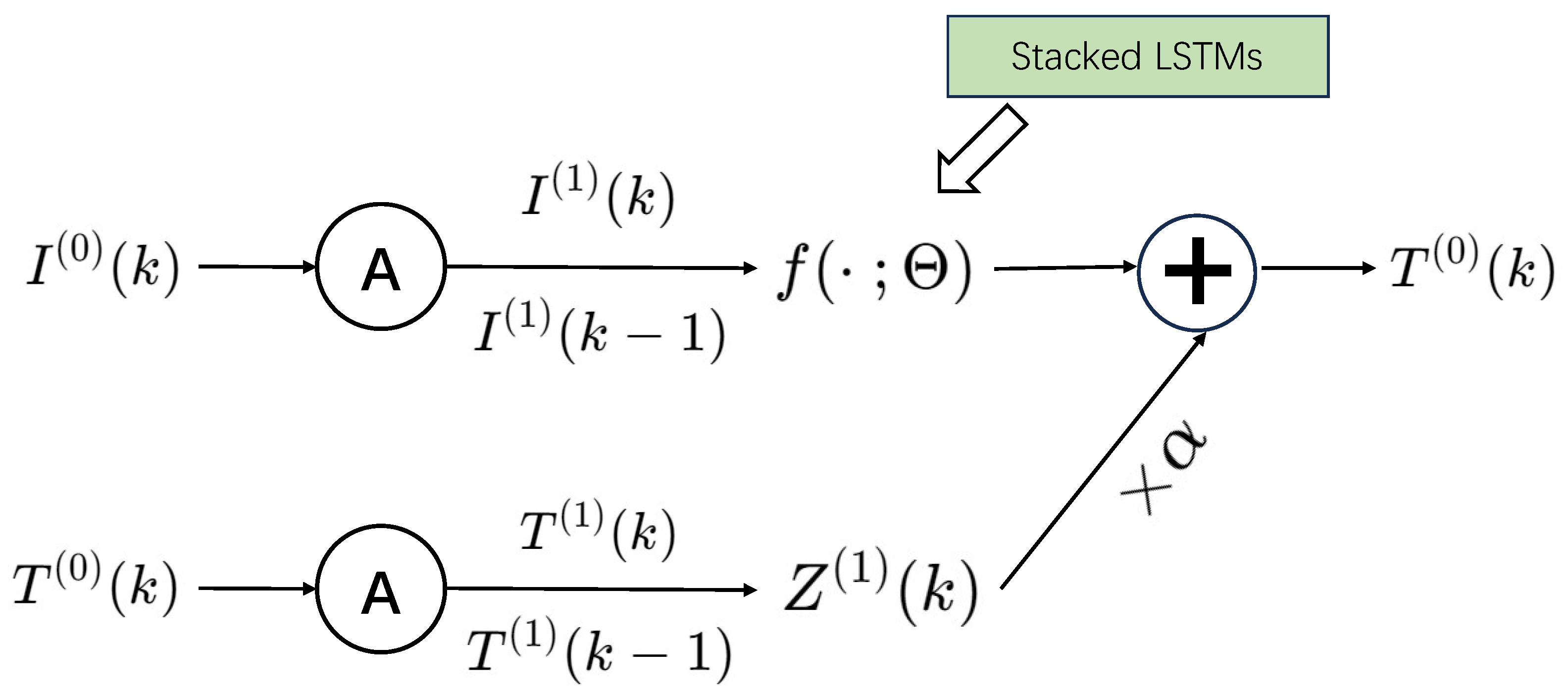
2.2. The Proposed Hybrid Grey System Model Based on Stacked LSTM Layers
2.3. Adam Algorithm for Training the Proposed Model
| Algorithm 1: Adam algorithm for training the hybrid grey system model | |||
| Input: (Equation (24)), learning rate l, max_iteration | |||
| Output: (Initialize the parameter set) | |||
| (Initialize the exponential decay rate) | |||
| (Initialize the exponential decay rate) | |||
| (Initialize the small constant) | |||
| (Initialize the moment) | |||
| (Initialize the moment) | |||
| (Initialize the number of iterations) | |||
| 1 | while do | ||
| 2 | iteration = iteration + 1; | ||
| 3 | Equation (26); (Calculate the objective function gradient) | ||
| 4 | Equation (29); (Calculate the first and second moment) | ||
| 5 | Equation (30); (Calculate the bias-corrected first and second moment) | ||
| 6 | Equation (31); (Update the parameters) | ||
| 7 | end | ||
| 8 | return (Resulting parameters) | ||
2.4. Grid Search Algorithm for Tuning Parameters of the Proposed Model
2.5. The Proposed Complete Forecasting Process
| Algorithm 2: Complete forecasting process of the GM-ResNet | |||
| Input: Training input: | |||
| Number of neurons L, learning rate l and max_iteration | |||
| Number of LSTM layers z; | |||
| Output: | |||
| ; | |||
| 1 | Equation (32); (Use GreySLstm-M1 or M2 to select the best ) | ||
| 2 | while do | ||
| 3 | ← Algorithm 1; (Use Algorithm 1 to train the model) | ||
| 4 | end | ||
| 5 | for to do | ||
| 6 | ← Equations (22) and (8); (Forecast by using the response function and 1-IAGO) | ||
| 7 | end | ||
| Result: | |||
3. Application
3.1. Data Collection
3.2. Selection of Comparison Models and Assessment Criteria
3.3. Case 1: Henan’s Coal Consumption
3.4. Case 2: Henan’s Electricity Consumption
3.5. Case 3: Henan’s Gasoline Consumption
3.6. Discussions
Analysis of the Performance of the Models on Real-World Cases
3.7. Analysis of the Indicator Optimization of the Proposed Model
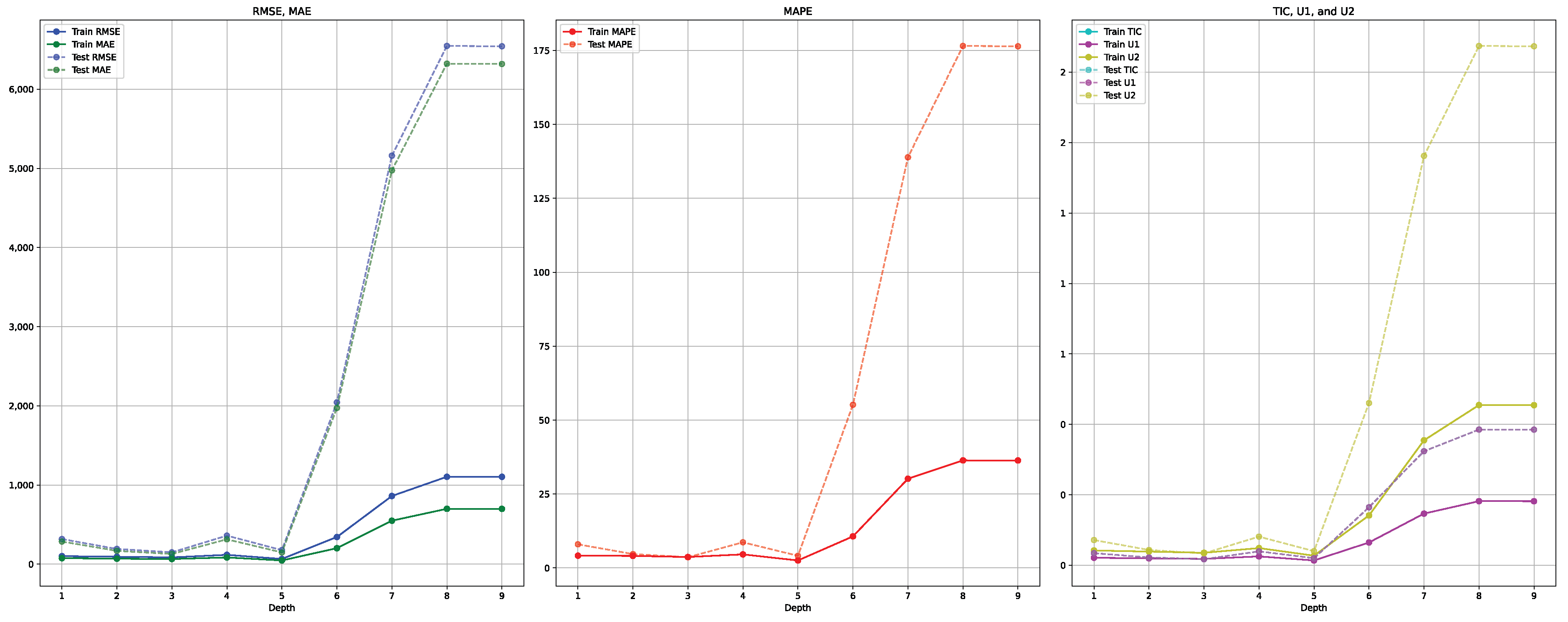
Evaluating GreySLstm Performance with Different Numbers of LSTM Layers
4. Conclusions
4.1. Paper Structure Overview
4.2. Main Findings and Contributions
4.3. Analysis of Potential Limitations of the Model
4.4. Recommendations for Model Enhancement
4.5. Future Research Directions
Author Contributions
Funding
Data Availability Statement
Conflicts of Interest
References
- Deng, J. Grey fuzzy forecast and control for grain. J. Huazhong Univ. Sci. Technol. Med. Sci. 1983, 2, 1–8. [Google Scholar]
- Deng, J. Grey dynamic model and its application in the long-term forecasting output of grain. Discov. Nat. 1984, 3, 37–45. (In Chinese) [Google Scholar]
- Xie, N.-M.; Liu, S.-F.; Yang, Y.-J.; Yuan, C.-Q. On novel grey forecasting model based on non-homogeneous index sequence. Appl. Math. Model. 2013, 37, 5059–5068. [Google Scholar] [CrossRef]
- Wang, Z.X.; Wang, Z.W.; Li, Q. Forecasting the industrial solar energy consumption using a novel seasonal GM (1, 1) model with dynamic seasonal adjustment factors. Energy 2020, 200, 117460. [Google Scholar] [CrossRef]
- Wu, W.; Ma, X.; Zhang, Y.; Li, W.; Wang, Y. A novel conformable fractional non-homogeneous grey model for forecasting carbon dioxide emissions of BRICS countries. Sci. Total. Environ. 2020, 707, 135447. [Google Scholar] [CrossRef]
- Liu, L.; Wu, L. Forecasting the renewable energy consumption of the European countries by an adjacent non-homogeneous grey model. Appl. Math. Model. 2021, 89, 1932–1948. [Google Scholar] [CrossRef]
- Luo, D.; Wei, B.L. A unified treatment approach for a class of discrete grey forecasting models and its application. Syst. Eng.-Theory Pract. 2019, 39, 451–462. [Google Scholar]
- Zhou, W.; Wu, X.; Ding, S.; Pan, J. Application of a novel discrete grey model for forecasting natural gas consumption: A case study of Jiangsu Province in China. Energy 2020, 200, 117443. [Google Scholar] [CrossRef]
- Qian, W.; Sui, A. A novel structural adaptive discrete grey prediction model and its application in forecasting renewable energy generation. Expert Syst. Appl. 2021, 186, 115761. [Google Scholar] [CrossRef]
- Ding, S.; Dang, Y.G.; Xu, H. Construction and application of GM (1, N) based on control of dummy variables. Control Decis. 2018, 33, 309–315. [Google Scholar]
- Wang, J. The GM (1, N) Model for Mixed-frequency Data and Its Application in Pollutant Discharge Prediction. J. Grey Syst. 2018, 30, 97. [Google Scholar]
- Luo, D.; An, Y.M.; Wang, X.L. Time-delayed accumulative TDAGM (1, N, t) model and its application in grain production. Control Decis. 2021, 36, 2002–2012. [Google Scholar]
- He, Z.; Wang, Q.; Shen, Y.; Wang, Y. Discrete multivariate gray model based boundary extension for bi-dimensional empirical mode decomposition. Signal Process. 2013, 93, 124–138. [Google Scholar] [CrossRef]
- Ding, S. A novel discrete grey multivariable model and its application in forecasting the output value of China’s high-tech industries. Comput. Ind. Eng. 2019, 127, 749–760. [Google Scholar] [CrossRef]
- Ding, S.; Xu, N.; Ye, J.; Zhou, W.; Zhang, X. Estimating Chinese energy-related CO2 emissions by employing a novel discrete grey prediction model. J. Clean. Prod. 2020, 259, 120793. [Google Scholar] [CrossRef]
- Ma, X.; Liu, Z. The kernel-based nonlinear multivariate grey model. Appl. Math. Model. 2018, 56, 217–238. [Google Scholar] [CrossRef]
- Duan, H.; Wang, D.; Pang, X.; Liu, Y.; Zeng, S. A novel forecasting approach based on multi-kernel nonlinear multivariable grey model: A case report. J. Clean. Prod. 2020, 260, 120929. [Google Scholar] [CrossRef]
- Ma, X.; Deng, Y.; Ma, M. A novel kernel ridge grey system model with generalized Morlet wavelet and its application in forecasting natural gas production and consumption. Energy 2024, 287, 129630. [Google Scholar] [CrossRef]
- Shaikh, F.; Ji, Q.; Shaikh, P.H.; Mirjat, N.H.; Uqaili, M.A. Forecasting China’s natural gas demand based on optimised nonlinear grey models. Energy 2017, 140, 941–951. [Google Scholar] [CrossRef]
- Xiao, Q.; Gao, M.; Xiao, X.; Goh, M. A novel grey Riccati–Bernoulli model and its application for the clean energy consumption prediction. Eng. Appl. Artif. Intell. 2020, 95, 103863. [Google Scholar] [CrossRef]
- Mao, S.; Zhu, M.; Wang, X.; Xiao, X. Grey–Lotka–Volterra model for the competition and cooperation between third-party online payment systems and online banking in China. Appl. Soft Comput. 2020, 95, 106501. [Google Scholar] [CrossRef]
- Ma, X.; Xie, M.; Suykens, J.A.K. A novel neural grey system model with Bayesian regularization and its applications. Neurocomputing 2021, 456, 61–75. [Google Scholar] [CrossRef]
- Liu, C.; Xu, Z.; Zhao, K.; Xie, W. Forecasting education expenditure with a generalized conformable fractional-order nonlinear grey system model. Heliyon 2023, 9, e16499. [Google Scholar] [CrossRef]
- Xie, D.; Li, X.; Duan, H. A novel nonlinear grey multivariate prediction model based on energy structure and its application to energy consumption. Chaos Solitons Fractals 2023, 173, 113767. [Google Scholar] [CrossRef]
- Wei, B.; Yang, L.; Xie, N. Nonlinear grey Bernoulli model with physics-preserving Cusum operator. Expert Syst. Appl. 2023, 229, 120466. [Google Scholar] [CrossRef]
- Zhao, H.; Guo, S. An optimized grey model for annual power load forecasting. Energy 2016, 107, 272–286. [Google Scholar] [CrossRef]
- Jin, M.; Zhou, X.; Zhang, Z.M.; Tentzeris, M.M. Short-term power load forecasting using grey correlation contest modeling. Expert Syst. Appl. 2012, 39, 773–779. [Google Scholar] [CrossRef]
- Zeng, B.; Luo, C. Forecasting the total energy consumption in China using a new-structure grey system model. Grey Syst. Theory Appl. 2017, 7, 194–217. [Google Scholar] [CrossRef]
- Guo, J.J.; Wu, J.Y.; Wang, R.Z. A new approach to energy consumption prediction of domestic heat pump water heater based on grey system theory. Energy Build. 2011, 43, 1273–1279. [Google Scholar] [CrossRef]
- Li, H.; Wu, Z.; Yuan, X.; Yang, Y.; He, X.; Duan, H. The research on modeling and application of dynamic grey forecasting model based on energy price-energy consumption-economic growth. Energy 2022, 257, 124801. [Google Scholar] [CrossRef]
- Lei, M.; Feng, Z. A proposed grey model for short-term electricity price forecasting in competitive power markets. Int. J. Electr. Power Energy Syst. 2012, 43, 531–538. [Google Scholar] [CrossRef]
- Duan, H.; Pang, X. A novel grey prediction model with system structure based on energy background: A case study of Chinese electricity. J. Clean. Prod. 2023, 390, 136099. [Google Scholar] [CrossRef]
- Pandey, A.K.; Singh, P.K.; Nawaz, M.; Kushwaha, A.K. Forecasting of non-renewable and renewable energy production in India using optimized discrete grey model. Environ. Sci. Pollut. Res. 2023, 30, 8188–8206. [Google Scholar] [CrossRef]
- Zhao, X.; Ma, X.; Cai, Y.; Yuan, H.; Deng, Y. Application of a novel hybrid accumulation grey model to forecast total energy consumption of Southwest Provinces in China. Grey Syst. Theory Appl. 2023, 13, 629–656. [Google Scholar] [CrossRef]
- Yuan, H.; Ma, X.; Ma, M.; Ma, J. Hybrid framework combining grey system model with Gaussian process and STL for CO2 emissions forecasting in developed countries. Appl. Energy 2024, 360, 122824. [Google Scholar] [CrossRef]
- He, Q.; Ma, X.; Zhang, L.; Li, W.; Li, T. The nonlinear multi-variable grey Bernoulli model and its applications. Appl. Math. Model. 2024, 134, 635–655. [Google Scholar] [CrossRef]
- Hochreiter, S.; Schmidhuber, J. Long short-term memory. Neural Comput. 1997, 9, 1735–1780. [Google Scholar] [CrossRef]
- Huang, Z.; Xu, W.; Yu, K. Bidirectional LSTM-CRF models for sequence tagging. arXiv 2015, arXiv:1508.01991. [Google Scholar]
- Krause, B.; Lu, L.; Murray, I.; Renals, S. Multiplicative LSTM for sequence modelling. arXiv 2016, arXiv:1609.07959. [Google Scholar]
- Shi, X.; Chen, Z.; Wang, H.; Yeung, D.-Y.; Wong, W.-K.; Woo, W.-C. Convolutional LSTM network: A machine learning approach for precipitation nowcasting. Adv. Neural Inf. Process. Syst. 2015, 28. [Google Scholar] [CrossRef]
- Wang, K.; Hua, Y.; Huang, L.; Guo, X.; Liu, X.; Ma, Z.; Ma, R.; Jiang, X. A novel GA-LSTM-based prediction method of ship energy usage based on the characteristics analysis of operational data. Energy 2023, 282, 128910. [Google Scholar] [CrossRef]
- Lu, H.; Wu, J.; Ruan, Y.; Qian, F.; Meng, H.; Gao, Y.; Xu, T. A multi-source transfer learning model based on LSTM and domain adaptation for building energy prediction. Int. J. Electr. Power Energy Syst. 2023, 149, 109024. [Google Scholar] [CrossRef]
- Lu, Y.; Sheng, B.; Fu, G.; Luo, R.; Chen, G.; Huang, Y. Prophet-EEMD-LSTM based method for predicting energy consumption in the paint workshop. Appl. Soft Comput. 2023, 143, 110447. [Google Scholar] [CrossRef]
- Deng, T.F.; Gui, Y.; Yan, J.Y. Prediction and analysis of tunnel crown settlement based on grey system theory. Adv. Mater. Res. 2012, 490, 423–427. [Google Scholar] [CrossRef]
- Gers, F.A.; Schmidhuber, J.; Cummins, F. Learning to forget: Continual prediction with LSTM. Neural Comput. 2000, 12, 2451–2471. [Google Scholar] [CrossRef] [PubMed]
- Andrychowicz, M.; Denil, M.; Gomez, S.; Hoffman, M.W.; Pfau, D.; Schaul, T.; Shillingford, B.; De Freitas, N. Learning to learn by gradient descent by gradient descent. Adv. Neural Inf. Process. Syst. 2016, 29. [Google Scholar] [CrossRef]
- Amari, S. Backpropagation and stochastic gradient descent method. Neurocomputing 1993, 5, 185–196. [Google Scholar] [CrossRef]
- Kingma, D.P.; Ba, J. Adam: A method for stochastic optimization. arXiv 2014, arXiv:1412.6980. [Google Scholar]
- Wang, S.; Lu, T.; Hao, R.; Wang, F.; Ding, T.; Li, J.; He, X.; Guo, Y.; Han, X. An Identification Method for Anomaly Types of Active Distribution Network Based on Data Mining. IEEE Trans. Power Syst. 2023, 39, 5548–5560. [Google Scholar] [CrossRef]
- Duan, Y.; Zhao, Y.; Hu, J. An initialization-free distributed algorithm for dynamic economic dispatch problems in microgrid: Modeling, optimization and analysis. Sustain. Energy Grids Netw. 2023, 34, 101004. [Google Scholar] [CrossRef]
- Liu, S.; Forrest, J.Y.L. Grey Systems: Theory and Applications; Springer Science & Business Media: Berlin/Heidelberg, Germany, 2010. [Google Scholar]
- Chen, P.Y.; Yu, H.M. Foundation settlement prediction based on a novel NGM model. Math. Probl. Eng. 2014, 2014, 242809. [Google Scholar] [CrossRef]
- Xie, N.; Wang, R.; Chen, N. Measurement of shock effect following change of one-child policy based on grey forecasting approach. Kybernetes 2018, 47, 559–586. [Google Scholar] [CrossRef]
- Chen, C.I.; Chen, H.L.; Chen, S.P. Forecasting of foreign exchange rates of Taiwan’s major trading partners by novel nonlinear Grey Bernoulli model NGBM (1, 1). Commun. Nonlinear Sci. Numer. Simul. 2008, 13, 1194–1204. [Google Scholar] [CrossRef]
- Wu, L.; Liu, S.; Yao, L.; Yan, S.; Liu, D. Grey system model with the fractional order accumulation. Commun. Nonlinear Sci. Numer. Simul. 2013, 18, 1775–1785. [Google Scholar] [CrossRef]
- Duan, H.; Lei, G.R.; Shao, K. Forecasting crude oil consumption in China using a grey prediction model with an optimal fractional-order accumulating operator. Complexity 2018, 2018, 3869619. [Google Scholar] [CrossRef]
- Ding, Y.; Dang, Y. Forecasting renewable energy generation with a novel flexible nonlinear multivariable discrete grey prediction model. Energy 2023, 277, 127664. [Google Scholar] [CrossRef]
- Wu, L.-F.; Liu, S.-F.; Cui, W.; Liu, D.-L.; Yao, T.-X. Non-homogenous discrete grey model with fractional-order accumulation. Neural Comput. Appl. 2014, 25, 1215–1221. [Google Scholar] [CrossRef]
- Wu, W.; Ma, X.; Zeng, B.; Wang, Y.; Cai, W. Forecasting short-term renewable energy consumption of China using a novel fractional nonlinear grey Bernoulli model. Renew. Energy 2019, 140, 70–87. [Google Scholar] [CrossRef]
- Wu, L.; Liu, S.; Chen, H.; Zhang, N. Using a novel grey system model to forecast natural gas consumption in China. Math. Probl. Eng. 2015, 2015, 686501. [Google Scholar] [CrossRef]
- Xia, J.; Ma, X.; Wu, W.; Huang, B.; Li, W. Application of a new information priority accumulated grey model with time power to predict short-term wind turbine capacity. J. Clean. Prod. 2020, 244, 118573. [Google Scholar] [CrossRef]
- Zhou, W.; Zhang, H.; Dang, Y.; Wang, Z. New information priority accumulated grey discrete model and its application. Chin. J. Manag. Sci. 2017, 25, 140–148. [Google Scholar]
- Xie, N.M.; Liu, S.F. Research on the non-homogenous discrete grey model and its parameter’s properties. Syst. Eng. Electron. 2008, 5, 863–867. [Google Scholar]
- Xiang, X.; Liu, L.; Cao, J.; Zhang, P. Forecasting the installed wind capacity using a new information priority accumulated nonlinear grey Bernoulli model. In IOP Conference Series: Earth and Environmental Science; IOP Publishing: Bristol, UK, 2020; Volume 467, p. 012088. [Google Scholar]
- Drucker, H.; Burges, C.J.; Kaufman, L.; Smola, A.; Vapnik, V. Support vector regression machines. Adv. Neural Inf. Process. Syst. 1996, 9. [Google Scholar]
- Breiman, L. Random forests. Mach. Learn. 2001, 45, 5–32. [Google Scholar] [CrossRef]
- Popescu, M.-C.; Balas, V.E.; Perescu-Popescu, L.; Mastorakis, N. Multilayer perceptron and neural networks. WSEAS Trans. Circuits Syst. 2009, 8, 579–588. [Google Scholar]
- Chen, T.; He, T.; Benesty, M.; Khotilovich, V.; Tang, Y.; Cho, H.; Chen, K.; Mitchell, R.; Cano, I.; Zhou, T. Xgboost: Extreme gradient boosting. R Package Version 0.4-2. 2015. Available online: https://cran.r-project.org/web/packages/xgboost/vignettes/xgboost.pdf (accessed on 14 August 2024).
- O’Shea, K.; Nash, R. An introduction to convolutional neural networks. arXiv 2015, arXiv:1511.08458. [Google Scholar]
- Dey, R.; Salem, F.M. Gate-variants of gated recurrent unit (GRU) neural networks. In Proceedings of the 2017 IEEE 60th international midwest symposium on circuits and systems (MWSCAS), Boston, MA, USA, 6–9 August 2017; pp. 1597–1600. [Google Scholar]
- Kim, S.; Hong, S.; Joh, M.; Song, S.-K. Deeprain: Convlstm network for precipitation prediction using multichannel radar data. arXiv 2017, arXiv:1711.02316. [Google Scholar]
- Kim, T.Y.; Cho, S.B. Predicting residential energy consumption using CNN-LSTM neural networks. Energy 2019, 182, 72–81. [Google Scholar] [CrossRef]


| Name | Reference | Year | Model Structure | Parameter |
|---|---|---|---|---|
| GM | [51] | 2010 | / | |
| NGM | [52] | 2014 | / | |
| DGM | [53] | 2018 | / | |
| NDGM | [3] | 2013 | / | |
| BernoulliGM | [54] | 2008 | b | |
| FGM | [55] | 2013 | ||
| FNGM | [56] | 2018 | ||
| FNDGM | [57] | 2023 | ||
| FDGM | [58] | 2014 | ||
| FBernoulliGM | [59] | 2019 | b | |
| NIPGM | [60] | 2015 | ||
| NIPNGM | [61] | 2020 | ||
| NIPDGM | [62] | 2017 | ||
| NIPNDGM | [63] | 2008 | ||
| NIPBernoulliGM | [64] | 2020 | b |
| Full Name | Abbreviation | Reference | Year |
|---|---|---|---|
| Support vector regression | svr | [65] | 1996 |
| Long Short-Term Memory | lstm | [45] | 2000 |
| Random forest regression | rf | [66] | 2001 |
| Multilayer perceptron | mlp | [67] | 2009 |
| Extreme gradient boosting | xgb | [68] | 2015 |
| Convolution neural network | cnn | [69] | 2015 |
| Gated recurrent unit | gru | [70] | 2017 |
| Convolutional LSTM | convlstm | [71] | 2017 |
| CNN-LSTM | cnnlstm | [72] | 2019 |
| Full Name | Metrics | Equation |
|---|---|---|
| Root-mean-square error | RMSE | |
| Mean absolute error | MAE | |
| Mean Absolute Percentage Error | MAPE | |
| Theil’s inequality coefficient | TIC | |
| Theil’s U1 statistic | U1 | |
| Theil’s U2 statistic | U2 |
| Model | GreySLstm-M1 | GreySLstm-M2 | gru | rf | xgb | lstm | svr | |
|---|---|---|---|---|---|---|---|---|
| Training | RMSE | 490.3060 | 960.1925 | 928.6231 | 870.6966 | 1574.2322 | 811.1070 | 1566.8574 |
| MAE | 339.5045 | 609.2220 | 658.7882 | 518.2737 | 1352.1988 | 529.3345 | 1367.6741 | |
| MAPE | 1.8857 | 2.9844 | 4.6797 | 2.7050 | 11.1550 | 3.6196 | 11.9076 | |
| TIC | 0.0133 | 0.0260 | 0.0252 | 0.0238 | 0.0432 | 0.0221 | 0.0425 | |
| U1 | 0.0133 | 0.0260 | 0.0252 | 0.0238 | 0.0432 | 0.0221 | 0.0425 | |
| U2 | 0.0266 | 0.0522 | 0.0505 | 0.0473 | 0.0855 | 0.0441 | 0.0851 | |
| Test | RMSE | 928.6467 | 5323.7461 | 2507.0439 | 3073.1162 | 1661.8960 | 1651.8883 | 2308.4474 |
| MAE | 910.8103 | 5108.5371 | 2329.0432 | 2799.0660 | 1172.6112 | 1436.7536 | 2166.6322 | |
| MAPE | 4.1222 | 23.2868 | 10.6819 | 12.8810 | 5.5687 | 6.6503 | 9.7389 | |
| TIC | 0.0209 | 0.1066 | 0.0532 | 0.0645 | 0.0362 | 0.0357 | 0.0540 | |
| U1 | 0.0209 | 0.1066 | 0.0532 | 0.0645 | 0.0362 | 0.0357 | 0.0540 | |
| U2 | 0.0414 | 0.2373 | 0.1117 | 0.1370 | 0.0741 | 0.0736 | 0.1029 | |
| Model | cnn | mlp | cnnlstm | convlstm | GM | NGM | DGM | |
| Training | RMSE | 2430.8773 | 3915.1753 | 861.2289 | 812.6766 | 3013.4610 | 2491.0085 | 3017.3331 |
| MAE | 2159.5672 | 3154.0362 | 597.2083 | 566.9696 | 2640.8209 | 2156.8366 | 2655.5472 | |
| MAPE | 14.2518 | 17.5495 | 3.1941 | 3.5721 | 17.3731 | 14.6886 | 17.6296 | |
| TIC | 0.0665 | 0.1152 | 0.0236 | 0.0221 | 0.0815 | 0.0691 | 0.0815 | |
| U1 | 0.0665 | 0.1152 | 0.0236 | 0.0221 | 0.0815 | 0.0691 | 0.0815 | |
| U2 | 0.1321 | 0.2127 | 0.0468 | 0.0442 | 0.1637 | 0.1353 | 0.1639 | |
| Test | RMSE | 11,761.7003 | 4033.4668 | 3381.0791 | 5542.6099 | 16,836.7866 | 9023.2598 | 16,728.2120 |
| MAE | 11,319.1136 | 3203.2006 | 3175.0204 | 5061.8062 | 16,073.4176 | 8607.2024 | 15,971.1954 | |
| MAPE | 51.5327 | 14.9912 | 14.5368 | 23.2690 | 73.2872 | 39.2627 | 72.8201 | |
| TIC | 0.2092 | 0.0839 | 0.0704 | 0.1110 | 0.2756 | 0.1687 | 0.2743 | |
| U1 | 0.2092 | 0.0839 | 0.0704 | 0.1110 | 0.2756 | 0.1687 | 0.2743 | |
| U2 | 0.5243 | 0.1798 | 0.1507 | 0.2471 | 0.7505 | 0.4022 | 0.7456 | |
| Model | NDGM | BernoulliGM | FGM | FNGM | FNDGM | FDGM | FBernoulliGM | |
| Training | RMSE | 2403.2727 | 5532.4287 | 4248.0164 | 4070.0333 | 2318.3493 | 4003.4205 | 6202.7378 |
| MAE | 2120.1498 | 4954.7318 | 3574.8920 | 3599.8241 | 1948.7597 | 3384.7620 | 5537.3872 | |
| MAPE | 15.0650 | 36.3972 | 30.5036 | 26.0696 | 12.7429 | 28.3588 | 41.8137 | |
| TIC | 0.0656 | 0.1669 | 0.1146 | 0.1150 | 0.0623 | 0.1086 | 0.1903 | |
| U1 | 0.0656 | 0.1669 | 0.1146 | 0.1150 | 0.0623 | 0.1086 | 0.1903 | |
| U2 | 0.1306 | 0.3006 | 0.2308 | 0.2211 | 0.1260 | 0.2175 | 0.3370 | |
| Test | RMSE | 9081.4995 | 1671.9496 | 3807.3586 | 6217.6065 | 11,715.2465 | 3689.2512 | 2269.5763 |
| MAE | 8708.0001 | 1383.7527 | 3298.5991 | 5447.6971 | 11,347.7484 | 3197.6934 | 2226.4167 | |
| MAPE | 39.6817 | 6.0014 | 15.2810 | 25.1836 | 51.5896 | 14.8132 | 9.9161 | |
| TIC | 0.1695 | 0.0363 | 0.0791 | 0.1235 | 0.2084 | 0.0768 | 0.0482 | |
| U1 | 0.1695 | 0.0363 | 0.0791 | 0.1235 | 0.2084 | 0.0768 | 0.0482 | |
| U2 | 0.4048 | 0.0745 | 0.1697 | 0.2771 | 0.5222 | 0.1644 | 0.1012 | |
| Model | NIPGM | NIPNGM | NIPDGM | NIPNDGM | NIPBernoulliGM | |||
| Training | RMSE | 4317.6857 | 3141.6617 | 4127.4823 | 2429.1336 | 3457.6183 | ||
| MAE | 3704.4585 | 2639.5239 | 3531.0537 | 1970.3929 | 2963.5155 | |||
| MAPE | 31.4827 | 16.0038 | 29.7322 | 11.6506 | 23.9604 | |||
| TIC | 0.1171 | 0.0886 | 0.1121 | 0.0656 | 0.0996 | |||
| U1 | 0.1171 | 0.0886 | 0.1121 | 0.0656 | 0.0996 | |||
| U2 | 0.2346 | 0.1707 | 0.2243 | 0.1320 | 0.1879 | |||
| Test | RMSE | 5153.0724 | 11,050.5598 | 3907.2315 | 13,174.3111 | 23,210.8592 | ||
| MAE | 4600.4453 | 10,461.0367 | 3395.0718 | 12,732.8356 | 18,689.1563 | |||
| MAPE | 21.2189 | 47.7791 | 15.7211 | 57.9115 | 87.2516 | |||
| TIC | 0.1042 | 0.1995 | 0.0810 | 0.2286 | 0.6128 | |||
| U1 | 0.1042 | 0.1995 | 0.0810 | 0.2286 | 0.6128 | |||
| U2 | 0.2297 | 0.4926 | 0.1742 | 0.5872 | 1.0346 |
| Model | GreySLstm-M1 | GreySLstm-M2 | gru | rf | xgb | lstm | svr | |
|---|---|---|---|---|---|---|---|---|
| Training | RMSE | 37.4968 | 63.6828 | 488.3888 | 34.8961 | 145.2803 | 295.4851 | 181.7269 |
| MAE | 28.8925 | 42.0938 | 220.5750 | 25.8150 | 121.5278 | 150.3027 | 156.6424 | |
| MAPE | 1.6761 | 2.0229 | 32.1378 | 1.4577 | 11.4320 | 20.5718 | 14.6458 | |
| TIC | 0.0096 | 0.0163 | 0.1259 | 0.0090 | 0.0378 | 0.0763 | 0.0468 | |
| U1 | 0.0096 | 0.0163 | 0.1259 | 0.0090 | 0.0378 | 0.0763 | 0.0468 | |
| U2 | 0.0193 | 0.0328 | 0.2514 | 0.0180 | 0.0748 | 0.1521 | 0.0935 | |
| Test | RMSE | 115.3096 | 200.4789 | 421.2057 | 523.4443 | 772.2424 | 457.9253 | 129.5320 |
| MAE | 95.7251 | 148.0640 | 377.4322 | 480.7118 | 743.9410 | 414.9213 | 108.6905 | |
| MAPE | 2.7584 | 3.9858 | 10.3856 | 13.2748 | 20.7229 | 11.4350 | 3.1498 | |
| TIC | 0.0162 | 0.0288 | 0.0627 | 0.0791 | 0.1215 | 0.0685 | 0.0180 | |
| U1 | 0.0162 | 0.0288 | 0.0627 | 0.0791 | 0.1215 | 0.0685 | 0.0180 | |
| U2 | 0.0325 | 0.0564 | 0.1186 | 0.1474 | 0.2174 | 0.1289 | 0.0365 | |
| Model | cnn | mlp | cnnlstm | convlstm | GM | NGM | DGM | |
| Training | RMSE | 189.6547 | 118.7663 | 105.7004 | 47.3233 | 231.5212 | 165.9904 | 232.7358 |
| MAE | 142.9024 | 93.4915 | 75.3073 | 35.2646 | 192.6853 | 132.2427 | 193.8591 | |
| MAPE | 14.3022 | 6.1338 | 4.0891 | 2.3983 | 14.3749 | 9.9145 | 14.5544 | |
| TIC | 0.0490 | 0.0304 | 0.0267 | 0.0122 | 0.0586 | 0.0435 | 0.0589 | |
| U1 | 0.0490 | 0.0304 | 0.0267 | 0.0122 | 0.0586 | 0.0435 | 0.0589 | |
| U2 | 0.0976 | 0.0611 | 0.0544 | 0.0244 | 0.1192 | 0.0854 | 0.1198 | |
| Test | RMSE | 293.7241 | 331.2288 | 124.8711 | 448.6507 | 1213.7337 | 277.8937 | 1215.1447 |
| MAE | 270.8711 | 310.8389 | 104.1500 | 392.9850 | 1163.1175 | 246.7314 | 1164.8605 | |
| MAPE | 7.6876 | 8.8156 | 2.9615 | 10.9248 | 32.5157 | 6.9568 | 32.5664 | |
| TIC | 0.0398 | 0.0447 | 0.0175 | 0.0598 | 0.1464 | 0.0378 | 0.1466 | |
| U1 | 0.0398 | 0.0447 | 0.0175 | 0.0598 | 0.1464 | 0.0378 | 0.1466 | |
| U2 | 0.0827 | 0.0933 | 0.0352 | 0.1263 | 0.3417 | 0.0782 | 0.3421 | |
| Model | NDGM | BernoulliGM | FGM | FNGM | FNDGM | FDGM | FBernoulliGM | |
| Training | RMSE | 152.1839 | 301.4826 | 268.4222 | 147.0146 | 136.9840 | 472.5171 | 263.7041 |
| MAE | 131.1087 | 266.4801 | 225.9895 | 110.9666 | 104.1567 | 376.2808 | 232.4938 | |
| MAPE | 10.3028 | 21.8860 | 19.2908 | 5.8802 | 6.6519 | 37.5129 | 18.9998 | |
| TIC | 0.0392 | 0.0822 | 0.0662 | 0.0381 | 0.0348 | 0.1151 | 0.0713 | |
| U1 | 0.0392 | 0.0822 | 0.0662 | 0.0381 | 0.0348 | 0.1151 | 0.0713 | |
| U2 | 0.0783 | 0.1552 | 0.1382 | 0.0757 | 0.0705 | 0.2432 | 0.1357 | |
| Test | RMSE | 340.3275 | 116.3608 | 773.9608 | 480.4346 | 473.8145 | 301.5636 | 149.3024 |
| MAE | 315.9793 | 107.1247 | 751.6470 | 459.6381 | 457.4457 | 270.4788 | 123.7991 | |
| MAPE | 8.9202 | 3.0525 | 21.1297 | 12.9606 | 12.9383 | 7.4586 | 3.3959 | |
| TIC | 0.0459 | 0.0163 | 0.0984 | 0.0635 | 0.0627 | 0.0442 | 0.0212 | |
| U1 | 0.0459 | 0.0163 | 0.0984 | 0.0635 | 0.0627 | 0.0442 | 0.0212 | |
| U2 | 0.0958 | 0.0328 | 0.2179 | 0.1353 | 0.1334 | 0.0849 | 0.0420 | |
| Model | NIPGM | NIPNGM | NIPDGM | NIPNDGM | NIPBernoulliGM | |||
| Training | RMSE | 214.9696 | 138.8300 | 232.3187 | 125.2973 | 272.0905 | ||
| MAE | 169.2131 | 109.0311 | 189.8683 | 90.8680 | 238.6010 | |||
| MAPE | 12.6166 | 6.0049 | 15.0377 | 5.2743 | 20.0758 | |||
| TIC | 0.0537 | 0.0361 | 0.0577 | 0.0319 | 0.0736 | |||
| U1 | 0.0537 | 0.0361 | 0.0577 | 0.0319 | 0.0736 | |||
| U2 | 0.1107 | 0.0715 | 0.1196 | 0.0645 | 0.1401 | |||
| Test | RMSE | 862.1933 | 404.1645 | 790.7576 | 429.9505 | 197.6275 | ||
| MAE | 836.4000 | 384.1215 | 768.0924 | 412.9963 | 150.0556 | |||
| MAPE | 23.4874 | 10.8571 | 21.5902 | 11.6904 | 4.0554 | |||
| TIC | 0.1085 | 0.0540 | 0.1004 | 0.0572 | 0.0283 | |||
| U1 | 0.1085 | 0.0540 | 0.1004 | 0.0572 | 0.0283 | |||
| U2 | 0.2427 | 0.1138 | 0.2226 | 0.1211 | 0.0556 |
| Model | GreySLstm-M1 | GreySLstm-M2 | gru | rf | xgb | lstm | svr | |
|---|---|---|---|---|---|---|---|---|
| Training | RMSE | 5.5247 | 8.7590 | 30.3996 | 9.4015 | 29.0164 | 17.2873 | 24.9984 |
| MAE | 3.3122 | 5.5920 | 19.1020 | 6.4205 | 25.1756 | 13.5572 | 23.0586 | |
| MAPE | 1.4747 | 2.2650 | 12.0591 | 2.9254 | 15.7324 | 7.8731 | 13.2535 | |
| TIC | 0.0128 | 0.0202 | 0.0711 | 0.0221 | 0.0666 | 0.0405 | 0.0593 | |
| U1 | 0.0128 | 0.0202 | 0.0711 | 0.0221 | 0.0666 | 0.0405 | 0.0593 | |
| U2 | 0.0257 | 0.0407 | 0.1413 | 0.0437 | 0.1348 | 0.0803 | 0.1162 | |
| Test | RMSE | 76.9153 | 96.7842 | 141.9118 | 278.8786 | 318.5326 | 94.8583 | 287.8411 |
| MAE | 65.5358 | 77.5446 | 126.7438 | 265.2736 | 306.6917 | 85.9361 | 254.5826 | |
| MAPE | 9.5421 | 11.1199 | 18.0005 | 38.6305 | 44.9456 | 12.3212 | 36.1240 | |
| TIC | 0.0566 | 0.0691 | 0.1168 | 0.2592 | 0.3079 | 0.0751 | 0.2640 | |
| U1 | 0.0566 | 0.0691 | 0.1168 | 0.2592 | 0.3079 | 0.0751 | 0.2640 | |
| U2 | 0.1142 | 0.1437 | 0.2108 | 0.4142 | 0.4731 | 0.1409 | 0.4275 | |
| Model | cnn | mlp | cnnlstm | convlstm | GM | NGM | DGM | |
| Training | RMSE | 89.2788 | 39.4255 | 35.1136 | 34.6697 | 40.1285 | 177.1090 | 40.0240 |
| MAE | 73.5071 | 29.2930 | 26.1866 | 26.6884 | 32.8573 | 122.6439 | 32.7378 | |
| MAPE | 43.4380 | 14.4692 | 13.2231 | 13.9887 | 17.4882 | 54.4627 | 17.4793 | |
| TIC | 0.2081 | 0.0922 | 0.0822 | 0.0811 | 0.0954 | 0.2982 | 0.0949 | |
| U1 | 0.2081 | 0.0922 | 0.0822 | 0.0811 | 0.0954 | 0.2982 | 0.0949 | |
| U2 | 0.4149 | 0.1832 | 0.1632 | 0.1611 | 0.1865 | 0.8230 | 0.1860 | |
| Test | RMSE | 462.0330 | 249.8680 | 104.4885 | 221.5902 | 168.8275 | 1536.1246 | 170.6696 |
| MAE | 453.9507 | 244.4299 | 95.2879 | 210.2770 | 164.6643 | 1349.0963 | 166.6187 | |
| MAPE | 67.3986 | 36.2082 | 14.6379 | 30.5910 | 24.8887 | 193.0584 | 25.1626 | |
| TIC | 0.5208 | 0.2275 | 0.0833 | 0.1959 | 0.1426 | 0.5397 | 0.1444 | |
| U1 | 0.5208 | 0.2275 | 0.0833 | 0.1959 | 0.1426 | 0.5397 | 0.1444 | |
| U2 | 0.6862 | 0.3711 | 0.1552 | 0.3291 | 0.2508 | 2.2815 | 0.2535 | |
| Model | NDGM | BernoulliGM | FGM | FNGM | FNDGM | FDGM | FBernoulliGM | |
| Training | RMSE | 34.0744 | 43.1875 | 37.6800 | 41.5449 | 42.8570 | 50.4337 | 36.0213 |
| MAE | 27.1748 | 33.1724 | 29.2709 | 34.4108 | 33.4238 | 40.2398 | 28.0154 | |
| MAPE | 14.6721 | 15.7012 | 16.7802 | 18.6444 | 16.0451 | 22.6073 | 16.1310 | |
| TIC | 0.0798 | 0.1050 | 0.0849 | 0.0978 | 0.1039 | 0.1174 | 0.0817 | |
| U1 | 0.0798 | 0.1050 | 0.0849 | 0.0978 | 0.1039 | 0.1174 | 0.0817 | |
| U2 | 0.1583 | 0.2007 | 0.1751 | 0.1931 | 0.1992 | 0.2344 | 0.1674 | |
| Test | RMSE | 197.0548 | 232.0179 | 217.0482 | 193.0278 | 241.6070 | 311.1789 | 362.4447 |
| MAE | 144.3595 | 229.0458 | 159.5841 | 189.3324 | 238.4823 | 305.2174 | 260.6160 | |
| MAPE | 20.1963 | 34.4236 | 22.2412 | 28.5918 | 35.7358 | 45.2670 | 35.9641 | |
| TIC | 0.1337 | 0.2076 | 0.1436 | 0.1666 | 0.2182 | 0.3001 | 0.2202 | |
| U1 | 0.1337 | 0.2076 | 0.1436 | 0.1666 | 0.2182 | 0.3001 | 0.2202 | |
| U2 | 0.2927 | 0.3446 | 0.3224 | 0.2867 | 0.3588 | 0.4622 | 0.5383 | |
| Model | NIPGM | NIPNGM | NIPDGM | NIPNDGM | NIPBernoulliGM | |||
| Training | RMSE | 40.0408 | 59.9252 | 33.8145 | 32.3140 | 37.7739 | ||
| MAE | 31.1999 | 42.8442 | 25.8625 | 28.0125 | 29.7247 | |||
| MAPE | 18.2299 | 24.0522 | 14.8879 | 16.1756 | 17.5189 | |||
| TIC | 0.0895 | 0.1439 | 0.0790 | 0.0760 | 0.0850 | |||
| U1 | 0.0895 | 0.1439 | 0.0790 | 0.0760 | 0.0850 | |||
| U2 | 0.1861 | 0.2785 | 0.1571 | 0.1502 | 0.1755 | |||
| Test | RMSE | 187.9752 | 107.3958 | 946.1340 | 7738.0291 | 443.3291 | ||
| MAE | 139.3251 | 87.2050 | 690.9050 | 4938.1195 | 311.9407 | |||
| MAPE | 19.4785 | 12.5335 | 94.8007 | 664.1561 | 42.8325 | |||
| TIC | 0.1268 | 0.0757 | 0.4286 | 0.8693 | 0.2582 | |||
| U1 | 0.1268 | 0.0757 | 0.4286 | 0.8693 | 0.2582 | |||
| U2 | 0.2792 | 0.1595 | 1.4052 | 11.4929 | 0.6585 |
| Model | vs. GreySLstm-M2 | vs. gru | vs. rf | vs. xgb | vs. lstm | vs. svr | vs. cnn |
|---|---|---|---|---|---|---|---|
| RMSE | 82.5565 | 62.9585 | 69.7816 | 44.1213 | 43.7827 | 59.7718 | 92.1045 |
| MAE | 82.1708 | 60.8934 | 67.4602 | 22.3263 | 36.6064 | 57.9619 | 91.9533 |
| MAPE | 82.2981 | 61.4092 | 67.9978 | 25.9755 | 38.0148 | 57.6727 | 92.0008 |
| TIC | 80.3937 | 60.6812 | 67.6062 | 42.2685 | 41.4517 | 61.3125 | 90.0117 |
| U1 | 80.3937 | 60.6812 | 67.6062 | 42.2685 | 41.4517 | 61.3125 | 90.0117 |
| U2 | 82.5565 | 62.9585 | 69.7816 | 44.1213 | 43.7827 | 59.7718 | 92.1045 |
| Model | vs. mlp | vs. cnnlstm | vs. convlstm | vs. GM | vs. NGM | vs. DGM | vs. NDGM |
| RMSE | 76.9765 | 72.5340 | 83.2453 | 94.4844 | 89.7083 | 94.4486 | 89.7743 |
| MAE | 71.5656 | 71.3132 | 82.0062 | 94.3334 | 89.4180 | 94.2972 | 89.5405 |
| MAPE | 72.5025 | 71.6429 | 82.2846 | 94.3753 | 89.5010 | 94.3392 | 89.6118 |
| TIC | 75.0942 | 70.3242 | 81.1786 | 92.4163 | 87.6138 | 92.3802 | 87.6714 |
| U1 | 75.0942 | 70.3242 | 81.1786 | 92.4163 | 87.6138 | 92.3802 | 87.6714 |
| U2 | 76.9765 | 72.5340 | 83.2453 | 94.4844 | 89.7083 | 94.4486 | 89.7743 |
| Model | vs. BernoulliGM | vs. FGM | vs. FNGM | vs. FNDGM | vs. FDGM | vs. FBernoulliGM | vs. NIPGM |
| RMSE | 44.4573 | 75.6092 | 85.0642 | 92.0732 | 74.8283 | 59.0828 | 81.9788 |
| MAE | 34.1782 | 72.3880 | 83.2808 | 91.9736 | 71.5166 | 59.0908 | 80.2017 |
| MAPE | 31.3125 | 73.0239 | 83.6314 | 92.0096 | 72.1720 | 58.4291 | 80.5729 |
| TIC | 42.4376 | 73.5743 | 83.0796 | 89.9698 | 72.7863 | 56.6203 | 79.9418 |
| U1 | 42.4376 | 73.5743 | 83.0796 | 89.9698 | 72.7863 | 56.6203 | 79.9418 |
| U2 | 44.4573 | 75.6092 | 85.0642 | 92.0732 | 74.8283 | 59.0828 | 81.9788 |
| Model | vs. NIPNGM | vs. NIPDGM | vs. NIPNDGM | vs. NIPBernoulliGM | |||
| RMSE | 91.5964 | 76.2326 | 92.9511 | 95.9991 | |||
| MAE | 91.2933 | 73.1726 | 92.8468 | 95.1265 | |||
| MAPE | 91.3724 | 73.7791 | 92.8819 | 95.2755 | |||
| TIC | 89.5263 | 74.1977 | 90.8570 | 96.5897 | |||
| U1 | 89.5263 | 74.1977 | 90.8570 | 96.5897 | |||
| U2 | 91.5964 | 76.2326 | 92.9511 | 95.9991 |
| Model | vs. GreySLstm-M2 | vs. gru | vs. rf | vs. xgb | vs. lstm | vs. svr | vs. cnn |
|---|---|---|---|---|---|---|---|
| RMSE | 42.4830 | 72.6239 | 77.9710 | 85.0682 | 74.8191 | 10.9799 | 60.7422 |
| MAE | 35.3488 | 74.6378 | 80.0868 | 87.1327 | 76.9293 | 11.9287 | 64.6603 |
| MAPE | 30.7929 | 73.4399 | 79.2205 | 86.6889 | 75.8773 | 12.4241 | 64.1183 |
| TIC | 43.9111 | 74.2029 | 79.5609 | 86.6971 | 76.4041 | 10.4043 | 59.4026 |
| U1 | 43.9111 | 74.2029 | 79.5609 | 86.6971 | 76.4041 | 10.4043 | 59.4026 |
| U2 | 42.4830 | 72.6239 | 77.9710 | 85.0682 | 74.8191 | 10.9799 | 60.7422 |
| Model | vs. mlp | vs. cnnlstm | vs. convlstm | vs. GM | vs. NGM | vs. DGM | vs. NDGM |
| RMSE | 65.1873 | 7.6571 | 74.2986 | 90.4996 | 58.5059 | 90.5106 | 66.1181 |
| MAE | 69.2043 | 8.0892 | 75.6415 | 91.7700 | 61.2027 | 91.7823 | 69.7053 |
| MAPE | 68.7097 | 6.8578 | 74.7508 | 91.5166 | 60.3493 | 91.5298 | 69.0766 |
| TIC | 63.8041 | 7.4294 | 72.9519 | 88.9578 | 57.2180 | 88.9685 | 64.7390 |
| U1 | 63.8041 | 7.4294 | 72.9519 | 88.9578 | 57.2180 | 88.9685 | 64.7390 |
| U2 | 65.1873 | 7.6571 | 74.2986 | 90.4996 | 58.5059 | 90.5106 | 66.1181 |
| Model | vs. BernoulliGM | vs. FGM | vs. FNGM | vs. FNDGM | vs. FDGM | vs. FBernoulliGM | vs. NIPGM |
| RMSE | 0.9034 | 85.1014 | 75.9989 | 75.6636 | 61.7628 | 22.7678 | 86.6260 |
| MAE | 10.6414 | 87.2646 | 79.1738 | 79.0740 | 64.6090 | 22.6771 | 88.5551 |
| MAPE | 9.6337 | 86.9452 | 78.7168 | 78.6801 | 63.0165 | 18.7709 | 88.2557 |
| TIC | 1.0207 | 83.5747 | 74.5354 | 74.1933 | 63.3875 | 23.8799 | 85.0928 |
| U1 | 1.0207 | 83.5747 | 74.5354 | 74.1933 | 63.3875 | 23.8799 | 85.0928 |
| U2 | 0.9034 | 85.1014 | 75.9989 | 75.6636 | 61.7628 | 22.7678 | 86.6260 |
| Model | vs. NIPNGM | vs. NIPDGM | vs. NIPNDGM | vs. NIPBernoulliGM | |||
| RMSE | 71.4696 | 85.4178 | 73.1807 | 41.6531 | |||
| MAE | 75.0795 | 87.5373 | 76.8218 | 36.2069 | |||
| MAPE | 74.5934 | 87.2237 | 76.4042 | 31.9820 | |||
| TIC | 70.0377 | 83.8895 | 71.7290 | 42.8803 | |||
| U1 | 70.0377 | 83.8895 | 71.7290 | 42.8803 | |||
| U2 | 71.4696 | 85.4178 | 73.1807 | 41.6531 |
| Model | vs. GreySLstm-M2 | vs. gru | vs. rf | vs. xgb | vs. lstm | vs. svr | vs. cnn |
|---|---|---|---|---|---|---|---|
| RMSE | 20.5290 | 45.8006 | 72.4198 | 75.8532 | 18.9155 | 73.2785 | 83.3528 |
| MAE | 15.4864 | 48.2927 | 75.2950 | 78.6314 | 23.7390 | 74.2575 | 85.5632 |
| MAPE | 14.1890 | 46.9899 | 75.2991 | 78.7697 | 22.5557 | 73.5852 | 85.8423 |
| TIC | 18.1348 | 51.5610 | 78.1745 | 81.6272 | 24.6273 | 78.5708 | 89.1368 |
| U1 | 18.1348 | 51.5610 | 78.1745 | 81.6272 | 24.6273 | 78.5708 | 89.1368 |
| U2 | 20.5290 | 45.8006 | 72.4198 | 75.8532 | 18.9155 | 73.2785 | 83.3528 |
| Model | vs. mlp | vs. cnnlstm | vs. convlstm | vs. GM | vs. NGM | vs. DGM | vs. NDGM |
| RMSE | 69.2176 | 26.3887 | 65.2894 | 54.4415 | 94.9929 | 54.9332 | 60.9676 |
| MAE | 73.1883 | 31.2234 | 68.8336 | 60.2004 | 95.1422 | 60.6672 | 54.6024 |
| MAPE | 73.6466 | 34.8124 | 68.8075 | 61.6611 | 95.0574 | 62.0784 | 52.7533 |
| TIC | 75.1257 | 32.0472 | 71.1178 | 60.3303 | 89.5159 | 60.8297 | 57.6863 |
| U1 | 75.1257 | 32.0472 | 71.1178 | 60.3303 | 89.5159 | 60.8297 | 57.6863 |
| U2 | 69.2176 | 26.3887 | 65.2894 | 54.4415 | 94.9929 | 54.9332 | 60.9676 |
| Model | vs. BernoulliGM | vs. FGM | vs. FNGM | vs. FNDGM | vs. FDGM | vs. FBernoulliGM | vs. NIPGM |
| RMSE | 66.8494 | 64.5630 | 60.1532 | 68.1651 | 75.2826 | 78.7787 | 59.0822 |
| MAE | 71.3875 | 58.9334 | 65.3859 | 72.5196 | 78.5282 | 74.8535 | 52.9620 |
| MAPE | 72.2804 | 57.0973 | 66.6266 | 73.2983 | 78.9205 | 73.4678 | 51.0122 |
| TIC | 72.7439 | 60.6075 | 66.0292 | 74.0691 | 81.1451 | 74.3007 | 55.3960 |
| U1 | 72.7439 | 60.6075 | 66.0292 | 74.0691 | 81.1451 | 74.3007 | 55.3960 |
| U2 | 66.8494 | 64.5630 | 60.1532 | 68.1651 | 75.2826 | 78.7787 | 59.0822 |
| Model | vs. NIPNGM | vs. NIPDGM | vs. NIPNDGM | vs. NIPBernoulliGM | |||
| RMSE | 28.3814 | 91.8706 | 99.0060 | 82.6505 | |||
| MAE | 24.8486 | 90.5145 | 98.6729 | 78.9909 | |||
| MAPE | 23.8675 | 89.9346 | 98.5633 | 77.7223 | |||
| TIC | 25.3015 | 86.7980 | 93.4915 | 78.0911 | |||
| U1 | 25.3015 | 86.7980 | 93.4915 | 78.0911 | |||
| U2 | 28.3814 | 91.8706 | 99.0060 | 82.6505 |
| LSTM Layer Number | 1 | 2 | 3 | 4 | 5 | 6 | 7 | 8 | 9 | ||
|---|---|---|---|---|---|---|---|---|---|---|---|
| Case 1 | RMSE | Train | 937.9942 | 851.0898 | 486.6038 | 844.6278 | 963.4058 | 3109.3818 | 10,351.4960 | 11,148.5194 | 11,152.6367 |
| Test | 5132.2100 | 3611.1851 | 1627.7841 | 3030.8841 | 5331.7715 | 19,477.6190 | 64,645.9305 | 68,870.8128 | 68,889.6010 | ||
| MAE | Train | 625.4415 | 521.0091 | 288.6944 | 547.3042 | 546.0693 | 1982.2757 | 6818.2956 | 7408.2859 | 7411.4835 | |
| Test | 4841.1397 | 3463.4200 | 1190.5096 | 2618.6103 | 5128.7763 | 18,726.4847 | 62,154.8233 | 66,233.5773 | 66,251.8598 | ||
| MAPE | Train | 3.1277 | 2.4315 | 1.3231 | 2.6728 | 2.4374 | 10.8775 | 39.6334 | 42.5158 | 42.5315 | |
| Test | 22.1315 | 15.7899 | 5.6178 | 12.0999 | 23.3665 | 85.2647 | 282.9392 | 301.4895 | 301.5725 | ||
| TIC | Train | 0.0254 | 0.0231 | 0.0132 | 0.0231 | 0.0260 | 0.0724 | 0.2276 | 0.2411 | 0.2412 | |
| Test | 0.1027 | 0.0747 | 0.0354 | 0.0635 | 0.1066 | 0.2361 | 0.5946 | 0.6105 | 0.6106 | ||
| U1 | Train | 0.0254 | 0.0231 | 0.0132 | 0.0231 | 0.0260 | 0.0724 | 0.2276 | 0.2411 | 0.2412 | |
| Test | 0.1027 | 0.0747 | 0.0354 | 0.0635 | 0.1066 | 0.2361 | 0.5946 | 0.6105 | 0.6106 | ||
| U2 | Train | 0.0510 | 0.0462 | 0.0264 | 0.0459 | 0.0523 | 0.1689 | 0.5624 | 0.6057 | 0.6060 | |
| Test | 0.2288 | 0.1610 | 0.0726 | 0.1351 | 0.2377 | 0.8682 | 2.8815 | 3.0698 | 3.0707 | ||
| Case 2 | RMSE | Train | 101.5587 | 94.1466 | 85.9299 | 118.1945 | 65.8725 | 343.2804 | 861.3843 | 1104.3757 | 1103.5302 |
| Test | 317.5203 | 192.0910 | 149.4493 | 360.5283 | 177.3545 | 2044.3780 | 5160.0670 | 6546.0611 | 6542.0924 | ||
| MAE | Train | 76.2756 | 69.4719 | 65.2312 | 85.1072 | 47.0495 | 202.2991 | 549.3752 | 699.6323 | 699.0246 | |
| Test | 286.1201 | 168.4210 | 128.8550 | 314.3367 | 148.3387 | 1973.5665 | 4974.8283 | 6322.1106 | 6318.2444 | ||
| MAPE | Train | 4.1573 | 4.0826 | 3.7143 | 4.5947 | 2.5382 | 10.6773 | 30.1723 | 36.3884 | 36.3614 | |
| Test | 8.0050 | 4.6901 | 3.6203 | 8.6849 | 4.1085 | 55.1810 | 138.8855 | 176.5324 | 176.4243 | ||
| TIC | Train | 0.0265 | 0.0245 | 0.0225 | 0.0313 | 0.0169 | 0.0807 | 0.1833 | 0.2274 | 0.2272 | |
| Test | 0.0429 | 0.0276 | 0.0213 | 0.0493 | 0.0249 | 0.2058 | 0.4046 | 0.4814 | 0.4813 | ||
| U1 | Train | 0.0265 | 0.0245 | 0.0225 | 0.0313 | 0.0169 | 0.0807 | 0.1833 | 0.2274 | 0.2272 | |
| Test | 0.0429 | 0.0276 | 0.0213 | 0.0493 | 0.0249 | 0.2058 | 0.4046 | 0.4814 | 0.4813 | ||
| U2 | Train | 0.0523 | 0.0485 | 0.0442 | 0.0608 | 0.0339 | 0.1767 | 0.4434 | 0.5685 | 0.5681 | |
| Test | 0.0894 | 0.0541 | 0.0421 | 0.1015 | 0.0499 | 0.5756 | 1.4528 | 1.8430 | 1.8419 | ||
| Case 3 | RMSE | Train | 38.5742 | 38.1353 | 31.8485 | 38.4768 | 38.4039 | 38.7443 | 38.8287 | 38.8505 | 38.6034 |
| Test | 208.8081 | 235.0953 | 206.5127 | 207.9963 | 206.1128 | 210.7499 | 211.8525 | 212.1576 | 208.7974 | ||
| MAE | Train | 30.9613 | 30.4737 | 25.0073 | 30.9819 | 30.8845 | 31.1706 | 31.2248 | 31.2383 | 31.0690 | |
| Test | 152.8418 | 171.6049 | 150.9447 | 152.2497 | 150.8776 | 154.2628 | 155.0598 | 155.2788 | 152.8170 | ||
| MAPE | Train | 18.5792 | 18.1695 | 14.8266 | 18.5924 | 18.5317 | 18.7202 | 18.7552 | 18.7637 | 18.6545 | |
| Test | 21.2923 | 23.8549 | 21.0333 | 21.2110 | 21.0236 | 21.4869 | 21.5960 | 21.6260 | 21.2890 | ||
| TIC | Train | 0.0867 | 0.0859 | 0.0720 | 0.0866 | 0.0864 | 0.0870 | 0.0872 | 0.0872 | 0.0868 | |
| Test | 0.1395 | 0.1535 | 0.1381 | 0.1391 | 0.1380 | 0.1406 | 0.1412 | 0.1414 | 0.1395 | ||
| U1 | Train | 0.0867 | 0.0859 | 0.0720 | 0.0866 | 0.0864 | 0.0870 | 0.0872 | 0.0872 | 0.0868 | |
| Test | 0.1395 | 0.1535 | 0.1381 | 0.1391 | 0.1380 | 0.1406 | 0.1412 | 0.1414 | 0.1395 | ||
| U2 | Train | 0.1793 | 0.1772 | 0.1480 | 0.1788 | 0.1785 | 0.1800 | 0.1804 | 0.1805 | 0.1794 | |
| Test | 0.3101 | 0.3492 | 0.3067 | 0.3089 | 0.3061 | 0.3130 | 0.3147 | 0.3151 | 0.3101 |
Disclaimer/Publisher’s Note: The statements, opinions and data contained in all publications are solely those of the individual author(s) and contributor(s) and not of MDPI and/or the editor(s). MDPI and/or the editor(s) disclaim responsibility for any injury to people or property resulting from any ideas, methods, instructions or products referred to in the content. |
© 2024 by the authors. Licensee MDPI, Basel, Switzerland. This article is an open access article distributed under the terms and conditions of the Creative Commons Attribution (CC BY) license (https://creativecommons.org/licenses/by/4.0/).
Share and Cite
Hao, Y.; Ma, X. A Hybrid Grey System Model Based on Stacked Long Short-Term Memory Layers and Its Application in Energy Consumption Forecasting. Processes 2024, 12, 1749. https://doi.org/10.3390/pr12081749
Hao Y, Ma X. A Hybrid Grey System Model Based on Stacked Long Short-Term Memory Layers and Its Application in Energy Consumption Forecasting. Processes. 2024; 12(8):1749. https://doi.org/10.3390/pr12081749
Chicago/Turabian StyleHao, Yiwu, and Xin Ma. 2024. "A Hybrid Grey System Model Based on Stacked Long Short-Term Memory Layers and Its Application in Energy Consumption Forecasting" Processes 12, no. 8: 1749. https://doi.org/10.3390/pr12081749