Abstract
This manuscript presents a model of a system implementing individual stages of production for long steel products resulting from rolling. The system encompasses the order registration stage, followed by production planning based on information about the billet inventory status, then offers the possibility of scheduling orders for the melt shop in the form of melt sequences, manages technological knowledge regarding the principles of sequencing, and utilizes machine learning and optimization methods in melt sequencing. Subsequently, production according to the implemented plan is monitored using IoT and vision tracking systems for ladle tracking. During monitoring, predictions of energy demand and energy consumption in LMS processes are made concurrently, as well as predictions of metal overheating at the CST station. The system includes production optimization at two levels: optimization of the heat sequence and at the production level through the prediction of heating time. Optimization models and machine learning tools, including mainly neural networks, are utilized. The system described includes key components: optimization models for sequencing heats using Ant Colony Optimization (ACO) algorithms and neural network-based prediction models for power-on time. The manuscript mainly focuses on process modeling issues rather than implementation or deployment details. Machine learning models have significantly improved process efficiency and quality; the optimization of planning has reduced sequencing plan execution time; and power-on time prediction models estimate the main ladle heating time with 97% precision, enabling precise production control and reducing overheating. The system serves as an example of implementing the concept of a cyber–physical system.
1. Introduction
The production of metal products using continuous casting has been the subject of numerous scientific and industrial studies for decades. This process is so energy-intensive and complex that it cannot be captured by a single model or information system. As in any industrial process, production has to be planned in advance; one must manage inventory and procurement, organize production, monitor processes, manage quality, and optimize production parameters. However, in this case, the process is on a massive scale, multi-stage, and energy-intensive, with costly and extensive inventories, variable demand, and extremely expensive storage of finished products. Maintaining quality is a significant challenge, and controlling parameters, especially scrap, is very difficult because it is often independent of the industrial plant. The process of melting and refining the metal bath, as a component of the production process, is still the subject of many industrial and scientific studies, in addition to efforts to control other elements such as production planning or further casting and rolling processes of steel. Most of the studies described in the literature focus on three stages of steel production: steel melting in the electric arc furnace (EAF—Electric Arc Furnace) [1], refining in LMS devices (Ladle Metallurgical Station) [2], and continuous casting of steel on Continuous Casters (CC) [3]. The analysis of heat losses in ladles has been the subject of publications related to ladle construction. Studies can be found on determining the optimal parameters of the ladle lining to minimize energy consumption [4].
The study of the relationships of variables in energy consumption models and their impact on energy consumption remains a topic of many publications and continues to interest researchers [5,6,7]. Developed models, including those using machine learning, usually rely on small data sets and carefully selected materials [8,9,10]. Numerical modeling has also been a developing research direction for years [11,12]. It is challenging to develop models for actual daily production that can significantly impact the energy intensity of the process due to the multivariable nature of dependencies. The main difficulty in modeling is the large number of factors with a small but statistically significant impact, the so-called weak learners. Most modeling techniques prefer a small number of strongly influencing factors (high correlation), which is the opposite in this process. Due to these difficulties, researchers most often deal with modeling under ideal conditions: on a selected subset of results from production chosen for one grade under established boundary conditions.
The studies presented in this article relate to an attempt to develop an information system that allows for monitoring and improving the management of the steelmaking process. The goal of the research is to enable precise evaluation of the necessary temperature of the main ladle at the moment of leaving the LMS station.
For this purpose, a cyber–physical system was implemented, allowing for the integration of both numerical modeling results and data from the measurement system of the production system, as well as the knowledge gathered in plant repositories. Cyber–physical systems (CPS) are systems of cooperating computational modules that are connected to the surrounding physical world and its ongoing processes, simultaneously providing and using services for data access and processing available in the plant network [13]. Such a system allows for a close connection of processes occurring in the physical world (production line) with computational, communication, and control systems in the cybernetic world [14,15]. The main goal of the research was to develop a globally innovative EAF-LMS-CC hybrid information system, integrated with the steel plant infrastructure, for the optimization and modeling of the steel billet production process. This solution significantly contributes to the quality of products by ensuring full control over the liquid steel temperature, including the overheating temperature.
In previous works by the authors, preliminary results of these research works have been presented, but only in selective aspects. For instance, in the work in [16], the informational model of hall monitoring and ladle image recognition was described, while in the work in [17], models predicting metal cooling during transport were presented. However, these aspects have not yet been described together, nor integrated with the planning component or prediction models for LMS power-on time, allowing for energy consumption assessment.
2. Materials and Methodology
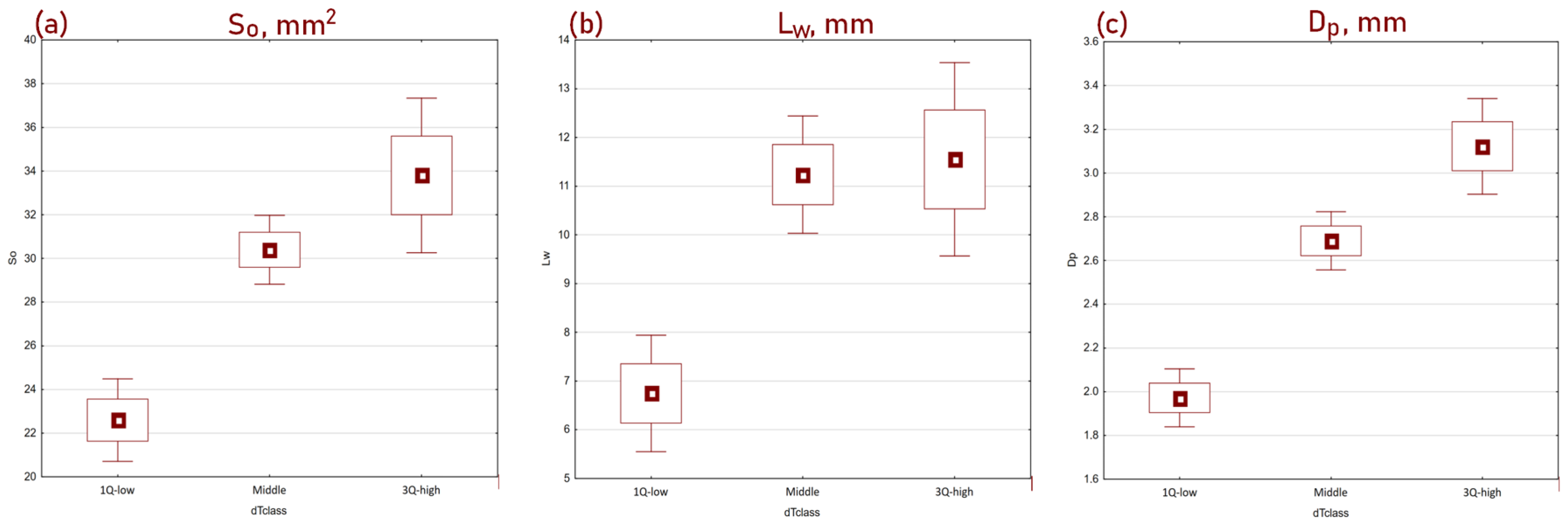
The CC process itself begins with loading scrap into the EAF furnace, where melting occurs. Then, the molten metal is poured into the main ladle, which is delivered to the LMS station. There, the metal bath is refined to achieve the desired chemical composition and temperature dependent on that composition, which affects the liquidus temperature of the given grade. The temperature at which the main ladle leaves the LMS station should be chosen so that its drop during transport, when it is not heated, ensures arrival at the CC station with a temperature 30–35 °C higher than the liquidus temperature, preventing the metal from freezing during casting. The risk associated with freezing the main ladle (150 t of liquid steel) or the crystallizer veins is too high to allow for mistakes. At the same time, the tendency to minimize this risk leads to overheating the main ladle at LMS. To secure against freezing that could occur if the transport to CC is prolonged or the casting of the previous melt takes longer than planned and the ladle has to wait in line, steel plant workers tend to overheat the ladle. Overheated metal loses its properties, its chemical composition changes, and unfavorable changes occur in the steel structure, leading to a decrease in billet quality. This has been confirmed by industrial studies showing that the number of defects increases with increasing overheating degree. In cases where overheating was higher than the third quartile (for each grade this value is different, but it is usually between 40 °C and 50 °C), or even above the median (35–40 °C), the number of defects such as surface area of the axial void (cavity) in the billet, the length of internal cracks, or deformation (rhombicity) of the billet increased significantly, as shown in Figure 1. Overheating of liquid steel also accelerates the wear of the refractory lining of the ladle furnace and the intermediate ladle and increases energy consumption.
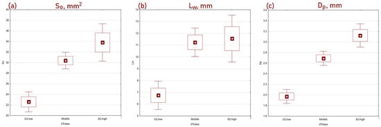
Figure 1.
Boxplots of three quality indicators categorized by the superheat quartile: (a) surface area of the axial void (cavity) in the billet (So, mm2); (b) the length of internal cracks (Lw, mm); (c) deformation (rhombicity) of the billet (Dp, mm).
However, even the knowledge of the risk of defect formation, as well as the risk of failing to meet the expected composition in the final product due to overheating of the ladle, is often not a sufficient factor to prevent overheating. This is because the cost of potential ladle freezing is significantly higher than the costs of repairing billets in the event of reduced quality. Even non-compliance with the chemical composition can be addressed, if necessary, by using the material for less quality-demanding rolled products, which is possible due to the varied production assortment.
To effectively counteract overheating, it is necessary to ensure constant and precise temperature monitoring in the ladle, as well as prediction of temperature changes after the LMS process is completed, and thus prediction of the ladle temperature during transport up to the moment of the anticipated start of casting into the tundish. An operator who trusts the system’s indications regarding the optimal temperature and the proper departure time from the LMS station will be more inclined to maintain the correct temperature, trusting that preventive overheating is not necessary. Reducing overheating, in addition to the demonstrated improvement in quality, can bring significant savings in energy consumption for refining and reheating the metal bath.
This article aims to present the results of work aimed at developing a system that allows for the integration of knowledge from process monitoring and production planning with feedback from production, which should enable the prediction of the correct temperature and the time of departure from the LMS.
One of the crucial elements of the system is the planning of heat sequences. The difficulty of this task lies in the need to simultaneously consider multiple boundary conditions arising from: (a) technological requirements regarding the materials that can be combined in the tundish, and consequently, the sequence of cast grades; (b) the number of heats in a sequence, defined as the maximum allowable number of heats for a given grade that ensures the safety of the refractory linings of the tundish; (c) the dimensions (cross-section and length) of the billet for a given order, resulting from the rolling mill order specifications; and (d) the order fulfillment date. At the same time, there is a need for optimization across several criteria: (1) the material (billets) intended for rolling must be ready on time due to the strict setup and rolling sequence requirements based on dimensions; (2) the number of heats in the sequence should be as large as possible to optimize the use of the tundish; and (3) minimum stock level—inventory optimization means keeping stocks as low as possible so that billets do not unnecessarily occupy storage yards, as this incurs additional storage costs as well as logistical and operational costs associated with handling and organizing.
The concept of scheduling is defined as the placement of activities in time given a certain number of conditions or constraints. It is closely related to the scheduling of tasks and operations that make up a given process (e.g., production process) [18].
Ant Colony Optimization (ACO) is an algorithm inspired by the behavior of ant colonies [19]. The algorithm seeks an optimal solution to a given problem by simulating how ants find the shortest path to a food source and mark it with pheromones. Ants that find shorter paths deposit pheromones more quickly, influencing the path choice of other ants. Pheromones evaporate on longer or less used paths, encouraging the exploration of the shortest known paths. ACO is primarily used for graph traversal in discrete spaces where the sequence of visited nodes matters. The algorithm assumes each edge in the graph has a weight that affects the rate of pheromone evaporation, which is convenient when knowledge about transitions is represented as graphs generated from transition matrices defined by technologists.
Genetic Algorithm (GA) is a method commonly used to generate high-quality solutions by employing mutation, crossover, and selection operators [20]. The evolution typically begins with randomly generated individuals and proceeds iteratively; each iteration is called a generation. In each generation, each new node is evaluated using a fitness function, a heuristic evaluation function of the chromosome—the set of parameters. The best nodes participate in crossover and mutation to produce offspring, thereby creating new nodes. The least fit nodes are removed. Genetic algorithms are fundamental methods for optimizing NP-hard problems, including the Traveling Salesman Problem (TSP), which involves finding the shortest path in a graph.
The literature presents various methods used in planning and scheduling production. The use of various variations of linear and integer programming [21,22], as well as heuristic and artificial intelligence methods, is popular [23].
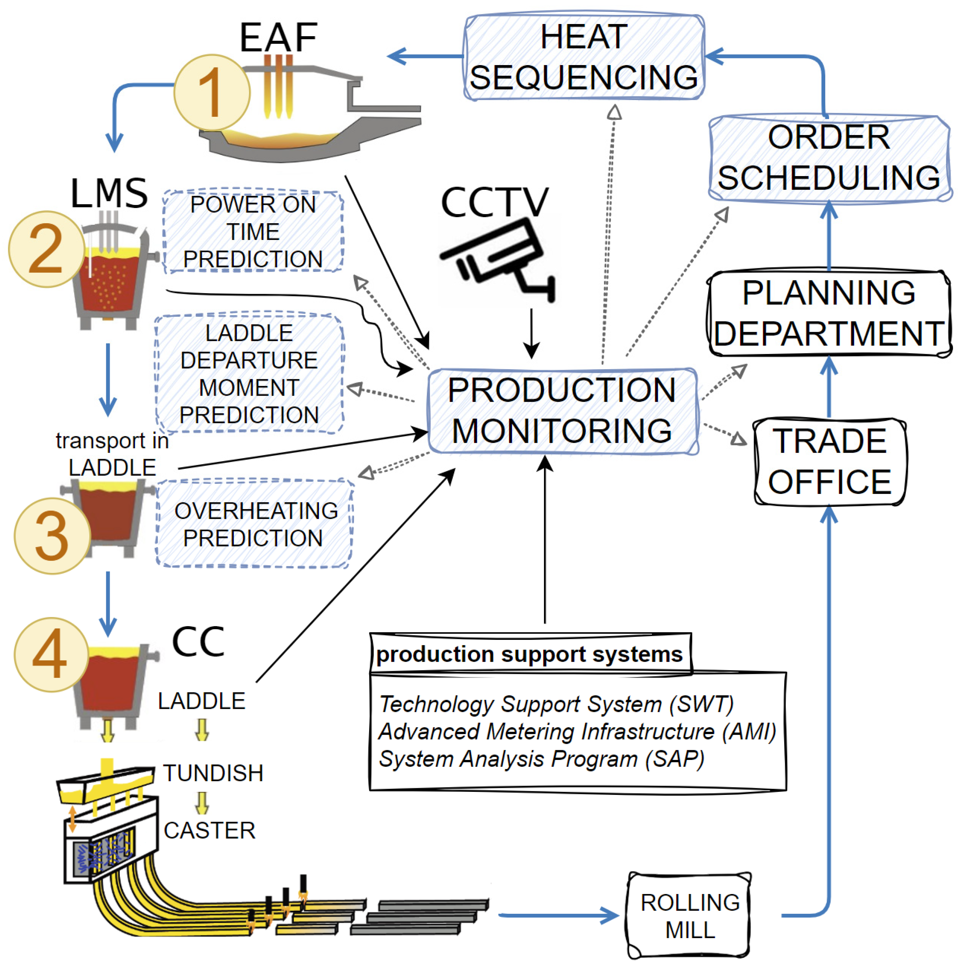
The elements of the system therefore include the following components: a production planning and scheduling system, which ensures the optimization of production plans; a system for monitoring the location of individual ladles in the melt shop hall; a system for monitoring process parameters and temperature; models for predicting casting time and energy consumption; and models for metal cooling during transport. This integrated system uses available, functioning data sources and knowledge in the plant, including measurement systems of devices (AMI—Advanced Metering Infrastructure), CCTV camera systems, technology support systems (SWT), SAP systems, and commercial data. The integration of these components and predictive models has made it possible to develop a production support system for the melt shop (Figure 2).

Figure 2.
SWP: production support system for melt shop—diagram of the production monitoring system in the continuous casting process using the plant’s IT infrastructure and ensuring the prediction of key information.
The two main sensory sources containing numerical data forming the AMI system—Advanced Metering Infrastructure—are the Level 1 and Level 2 systems.
Level 1 is a low-level hardware layer integrated directly with the controllers of devices involved in the production process (EAF-LMS-CC). It provides real-time parameters concerning the current state of these devices. Integration with this layer is based on a connection with the Siemens Simatic S7 400 controller, implemented through the Sharp7 library, which is a port of the Snap7 library in C#. Data obtained from this layer include the current temperature of the main ladle shell, the latest measurements of the liquid steel temperature, the current process duration at the EAF or LMS station, and the current amount of energy consumed at individual stations.
Level 2 is another sensory layer in the melt shop hall, which provides data on process parameters after processing the charge in the main ladle at various stages of the production process (EAF, LMS, CC). This layer provides additional data concerning the production process, covering the entire production plan and specific heats carried out in a given ladle (grade, sequence in the production process, charge mass, chemical composition, oxygen and carbon content, total processing time at a given station, melting process efficiency). This information complements the data from the Level 1 system, but is not delivered in real-time and appears in the system only after the ladle processing at a given station is completed. Numerical data from the Level 2 system are provided in the form of XML file reports, which are detected and parsed using FileWatcher tools, XSD, and standard C# libraries used for parsing XML documents.
The image processing component from CCTV performs two main functions: ladle detection and ladle number identification. In the course of work on the ladle detection problem, four different machine learning models were tested to verify their effectiveness—Mask-RCNN, MobileNet, YOLOv3, and its Tiny version. Mask-RCNN provided 96% effectiveness in detecting the ladle’s position. It was also noted that the effectiveness of ladle detection and ladle number identification slightly decreases in situations where smoke or sudden light flashes appear on the scene. This is a difficult case, as even the operator of the vision system has trouble recognizing the ladle number in such situations.
The integration of data from various sensor layers (Level 1, Level 2, CCTV) is realized in the system through a component that aggregates these data and makes them available to the metamodeling, optimization, and process monitoring components (via a mobile application). The exchange of information between these components is based on the open-source message broker RabbitMQ. The component monitoring the melt shop hall state considers the accuracy and reliability of data from individual components. Data from the Level 2 system have the highest priority (partially verified by the operator). These data are then supplemented with information on the current state of the process provided by the Level 1 layer (current data but without information on the overall process state). Data from the CCTV system allow for precise positioning of individual ladles within the hall, but is the least accurate—there are situations where a ladle is detected without recognizing its number or with an incorrect number. Corrections to the ladle numbering are made based on data from the Level 2 system, taking into account the sequencing of the ladle processing scheme in the melt shop hall based on the daily production schedule obtained from the planning component.
3. Level 1 Optimization: Algorithms for Casting Scheduling and Sequences
Scheduling orders for the melt shop involves determining the optimal sequence of orders for heats to be carried out within the designated rolling campaigns. This means optimization on three levels:
- Rolling mill: To ensure uptime operation by providing the required material for rolling.
- Melt shop: To maximize sequence length and minimize transitional billets, thereby reducing production costs by maximizing the use of tundishes and main ladles.
- Warehouse: To maintain a minimum stock level since storing billets is expensive, and their subsequent use may pose logistical difficulties due to their size, weight, and storage method.
The permissible sequence of individual materials in the tundish, where the heats from the main ladles are mixed, is described in the knowledge base. If it is not possible to plan a material sequence (technological recipes) that can be sequentially planned due to the lack of appropriate orders, the sequence must be interrupted and the tundish replaced. This generates additional costs and time needed for the rebuild. Sequences are planned to maximize tundish utilization and minimize the number of technological recipe transitions that cannot be sequenced.
In the research work, the possibility of using nature-inspired optimization algorithms in the process of optimizing heat sequences was analyzed. Specifically, the feasibility of applying Genetic Algorithms (GA) and Ant Colony Optimization (ACO) was considered. The feasibility analysis of the application and usefulness of these algorithms took into account important selection criteria for the tools:
Step 1: Based on the input data, obtain the current list of orders arranged according to the campaign plan—the time criterion.
Step 2: Parse and acquire the transition matrix (rules of technological recipes succession). The input data are then processed into a graphical form.
Step 3: The algorithm optimizes within the constraints set by the boundary conditions: the list of orders considering the execution time and possible connections of technological recipes into sequences, giving us a discrete search space for optimal solutions.
Considering the criteria in the analysis, individual algorithms could be evaluated based on the benefits of their application. Swarm algorithms that mimic the behaviors of fish schools, bee swarms, or bird flocks do not store any additional information.
Two algorithms were selected for implementation: the Ant Colony Optimization (ACO) algorithm and the Genetic Algorithm (GA). In both cases, the input data, apart from the algorithms’ hyperparameters, were graphs of permissible transitions between species/technological instructions. These graphs were generated based on campaign plans and transition matrices. Due to their size, they pose a challenge in terms of visualization (Figure 3).
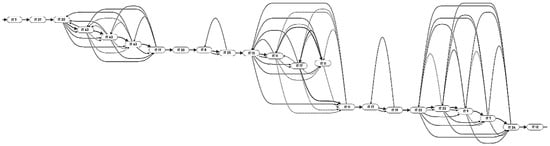
Figure 3.
A sample segment of heating sequences obtained using the ACO algorithm. Each node represents the number of a technological instruction (IT) that can be connected with others ‘at no cost’ to the same type of node or between or between grades, which can be combined according to the transition matrix, described by a different type of transition with a different cost.
In these graphs, each node represents one heat of a separate IT (technological instruction/recipe). Batches of the same species (instruction—IT) can be connected ‘at no cost’ to the same type of node. Between different grades (IT), connections may exist according to the transition matrix, described by a different type of transition with a different cost.
In this case, none of the methods was directly able to provide a complete solution. The complexity of the process made it impossible to use only classic or heuristic scheduling algorithms (i.e., Ant Colony Optimization, Evolutionary Algorithms, Simulated Annealing, etc.); rule-based systems are also not suitable for such complex decision-making processes. Therefore, the solution had to take a hybrid form—the mechanism includes both elements of optimization (searching for connection graphs) and rule-based reasoning (steel rules).
Scheduling concerns two processes. Firstly, the Scheduler defines the rolling mill production plan (planning). This is a rough plan defining upcoming campaigns for each rolling mill line, specifying which products will be rolled on particular days and in what quantities. These campaigns provide salespeople with information on when customers can expect their orders to be fulfilled. The system uses this plan to organize the order list according to the rolling mill setup changeover frames (sequencing). This creates the rolling mill production schedule.
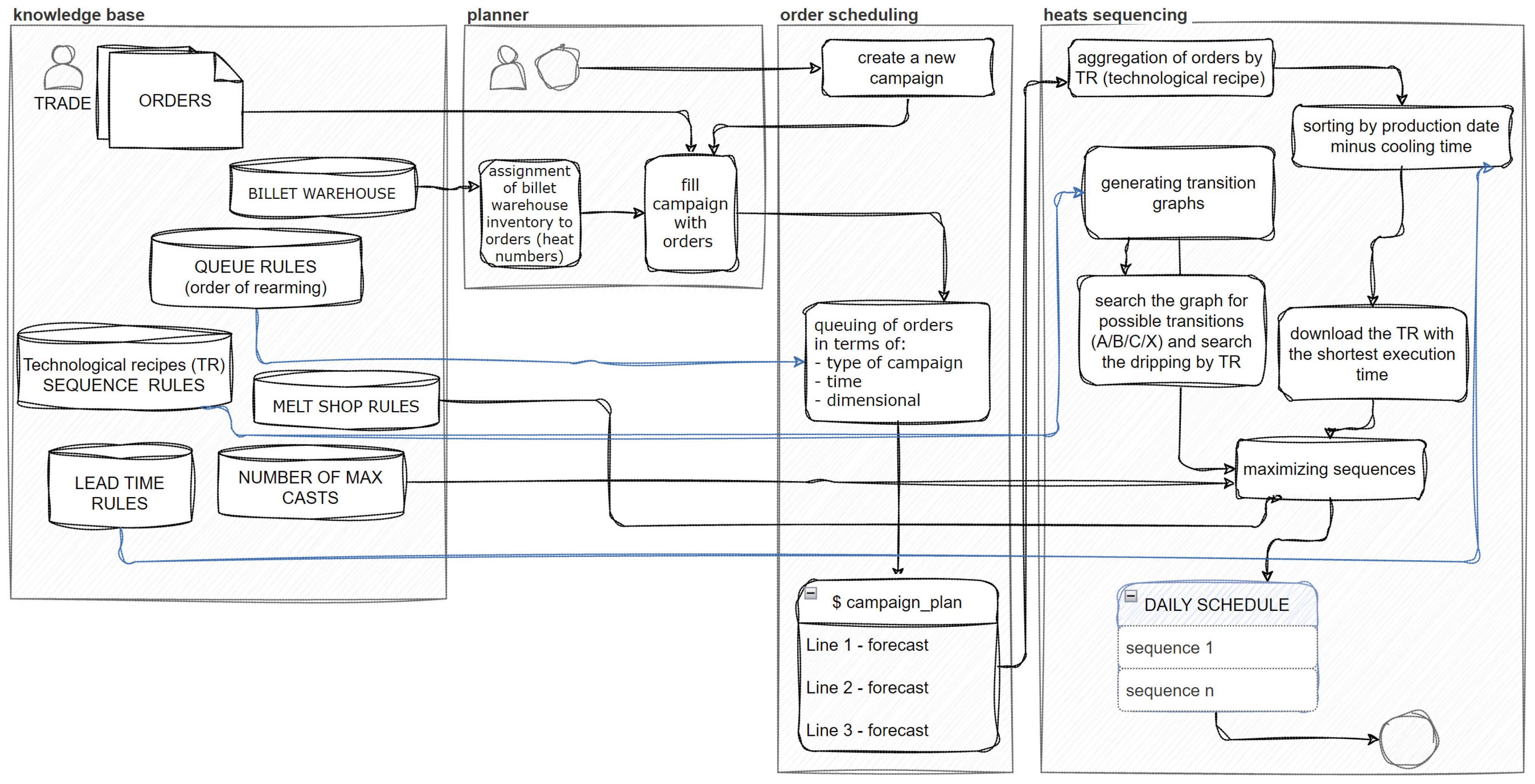
In the second stage, based on this rolling plan, the melt shop production plan (steelworks) is created to meet the material demand for rolling. Within the melt shop scheduling, the sequencing of heats for different materials also occurs. Each material is cast according to a specific technological recipe (Technological Recipes—TR), which constitutes a technological operation. Thus, the sequence of technological operations is a sequence of several (maximum twenty-three operations) consecutive, different technological instructions. The algorithm uses TR symbols; hence, the task of scheduling boils down to determining the sequence of TRs required in the order, considering boundary conditions in the form of rules. These rules were derived through knowledge engineering from technologists, which was the first stage of system development. The algorithm performs the task of creating sequences for specific steel grades and order sizes (tonnages) to achieve a feasible production sequence (Figure 4).
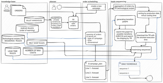
Figure 4.
The primary components of the process of planning and sequencing heats.
Regarding the optimization module, the inputs to the model are illustrated in Figure 4. These include: the order list from the SAP system; inventory levels from the SAP system; queue rules—rules for queuing resulting from mill retooling and defined by technologists; transition rules (rules for combining materials into sequences) defined in the knowledge base by technologists and mapped by the described system into graph form; and steelmaking rules defined by technologists from the melt shop that specify additional rules for ordering materials in the melting queue, the knowledge base on the maximum number of heats for a given material in a sequence, and the cooling time for the given material. The output of the model is the daily sequence plan for heats. Thus, one can determine: the number of heats per day, the melting time, and the degree of alignment of the actual plan with the ideal plan, as assessed by the lead technologist in terms of quality.
The algorithm’s main task in the proposed system is to determine sequences for specified steel grades while meeting boundary conditions in the form of permissible rules for transitions between grades. The developed system is based on knowledge engineering, meaning it is incremental and adaptable. Its learning mechanism relies on interaction with the system operator—either a technologist or planner. It is crucial to equip such tools with high-quality and accurate data representing solutions that have been tested and are expected for specific problems. The system operator should possess expertise in the field to provide necessary data during system operation.
The algorithm utilizes knowledge bases developed from technologists’ expertise. The primary base is a matrix of sequential connections between technological recipes (TRs), enabling the creation of rules for combining materials into sequences in the form of graph. Another essential base is the Maximum Number of Heats for each TR, which determines the maximum length of the heat sequence. Additionally, the Lead Time Margin Matrix is crucial, storing minimum cooling times required for each TR, which are added to the TR execution time. Historical melting times of specific materials, calculated from production data, serve as factual bases. The system also maintains configuration data and a database of steelmaking rules, influencing the scheduling format—for instance, avoiding single heats or alternating short and long sequences.
The system retrieves data from warehouses and the SAP system, where orders are stored. Orders are divided into 150-ton production orders for heats of specific grades (TRs), which in turn fill rolling campaigns, specifying the deadline for casting while considering cooling time. Daily aggregates of heat orders are then sequenced according to a transition matrix and the maximum number of melts per sequence. This step incorporates graph-based optimization of transitions to maximize the sequence. By monitoring the melt shop hall and collecting process data, the operator can verify plan execution and make adjustments as needed. Determining temporary plant preferences allows us to indicate operational strategies—maximizing tundish utilization (maximal sequences resulting in production above order baskets) or minimizing warehouse usage (production limited to ordered materials only). These modes can be switched depending on current market conditions, often in a cyclical manner.
The results of both implemented optimization algorithms are presented in Table 1. The Genetic Algorithm is much faster, but very far from the optimal solution. Its advantages are simplicity and speed of computation. The algorithm quickly finds a solution; however, the sequences it generates are very short, which means a large number of transitions and higher costs. The Ant Colony Algorithm takes significantly longer to calculate the shortest path, but provides better solutions. Longer sequences mean fewer transitions. The algorithm is much more inclined to connect TRs that do not require generating a transition. Its advantage is the inherent assessment of graph edges—such a cost assigned to the edges causes a preference for paths that guarantee better solutions, instead of the “blind” optimization using GA. The Ant Colony Algorithm was chosen for the final implementation. Despite the fact that the sequences generated by each algorithm matched the production plan by more than 95%, ACO gave better results from the perspective of a technologist’s real evaluation.

Table 1.
The results of the optimization algorithms.
Algorithm parameters were chosen experimentally.
ACO: number of ants: 10; evaporation rate (rho): 0.01; minimum pheromone value on an edge (Q): 2; Alpha (pheromone weight in decision making): 3; Beta (heuristic weight in decision making): 2.
GA: The genotype is a list of all graph nodes. The initial population consists of 50 individuals, each with a random genotype. In each iteration, 15 of the best-fitting individuals (with the lowest graph traversal cost) are selected. These 15 individuals proceed to the next iteration, along with 15 individuals created through mutation of the best-fitting individuals and 20 individuals created through mutation of 20 random individuals from the population. Mutation involves selecting a random length of the individual’s genotype and rearranging the genes in that segment randomly. The program keeps track of the best-fitting individual and checks in each iteration if a better-fitting individual has appeared. If so, the new one replaces the best. The process is repeated for 100 iterations.
This is Level 1 optimization. Next, Level 2 optimization is conducted: process parameters are optimized by monitoring the ladle metallurgy station’s (LMS) power-on-time and ladle departure time for the continuous caster (CC) station.
4. Level 2 Optimization: Optimizing Process Parameters
Level 2 optimization includes process control support based on predictions of key parameters. Figure 2 shows this in the left line of the process. At the LMS station, energy consumption is directly related to the residence time of the metal bath under current (power-on-time). This time is, of course, necessary to achieve the desired chemical composition; however, it is also somewhat influenced by the operator’s subjective belief about the temperature that should be achieved to safely transport the ladle to the CC station. This means the operator anticipates the temperature drop during transport and casting and ensures overheating at a level that only allows for cooling during transport and maintaining the required temperature during casting, while simultaneously preventing the vein from freezing—to bring the ladle to the appropriate temperature before the expected departure time. To increase the safety of this process, key information necessary to make the right decision about the desired temperature is secured: the liquidus temperature for a given steel grade, the predicted temperature drop during transport, the correct departure time from LMS so that the ladle does not have to wait before the tundish for casting, and the estimated dwell time under current at LMS (power-on-time) to ensure the ladle’s energy requirements are met.
Methods of prediction and modeling of cooling during transport were previously described in the work in [17]. Developed models, particularly neural networks, Classification and Regression Trees (CART), and predictive modules, were incorporated into the monitoring system of the melt shop. The models have been validated during ongoing production, and their effectiveness has been highly rated. Having a cooling model, the appropriate temperature allowance can be estimated, providing the moment when casting will begin.
The prediction of the casting start time is based on calculations derived from the known weight of metal in the tundish, the number of strands currently being cast in the caster, the casting speed of the strands, the cross-section of the strands (resulting from the billet sizes), and the density of steel. Therefore, the moment at which the tundish will reach a level that requires the start of casting the next ladle into the tundish can be calculated. At this point, the ladle must be ready on the turret. The travel time of the ladle from each of the two LMS stations is also known, allowing for the determination of when a given ladle should leave the respective LMS station.
The system, therefore, indicates how much time is left until the departure from the LMS. The operator’s role is to achieve the appropriate temperature within this time, which the system also suggests. Knowing the energy characteristics of the LMS furnace, the operator knows how long he should heat the ladle. However, the refining cycle is associated with episodes of heating (power-on-time) and argon stirring, as well as ladle holding episodes. How to alternate this cycle remains at the operator’s discretion. However, the system can suggest the optimal amount of time under power for the ladle to reach the desired temperature. Another implemented model is used for this purpose.
Power-on-Time Prediction
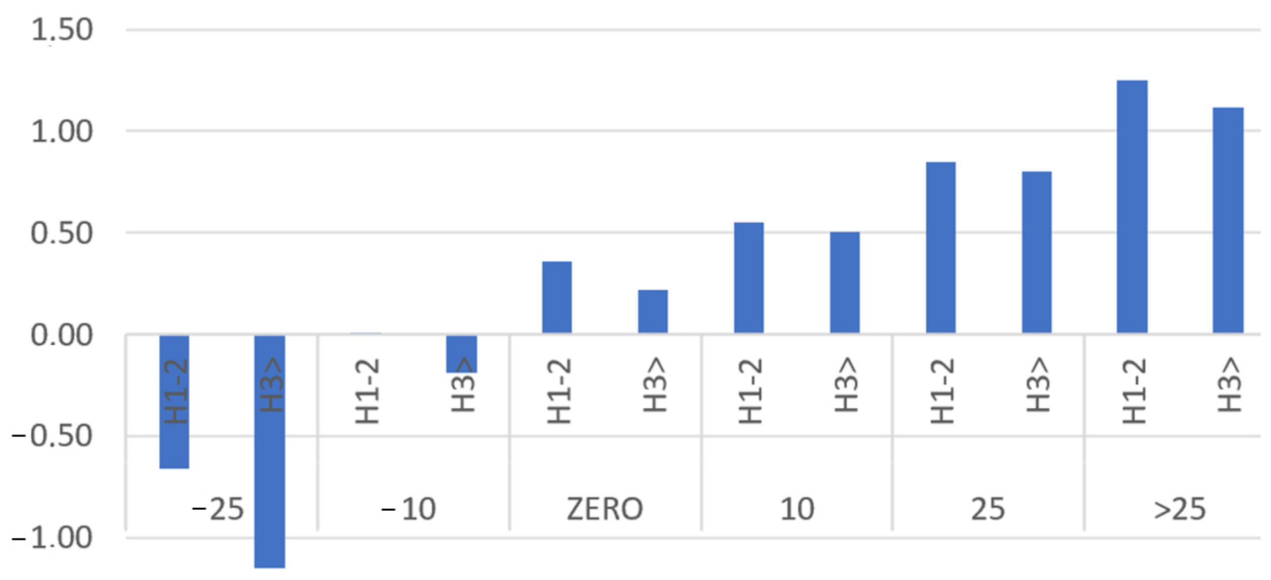
Predicting the optimal time to stay under current is not an easy task. This issue is related to the type of steel, the liquidus temperature, the chemical composition of the bath, the initial processing temperature in the LMS, the degree of mixing, the characteristics of the LMS device, the transport time to the CC, and also the sequence order (the significant impact of whether it is the first or second heat in the sequence). Research on historical data, totaling nearly 50,000 heats, indicated numerous deviations, records from non-routine operations, process disturbances, and measurement disruptions, which had to be iteratively filtered by examining the statistics of almost every process parameter. The production data allowed for the analysis of the energy consumption rate required to heat a metal bath by 1 °C per minute. Data analysis demonstrated that energy consumption for each 1 °C temperature increase varies during processing in the LMS. The energy consumed for each 1 °C temperature increase depends on the type of steel and, among other factors, the initial temperature as well as the sequence order (which also affects, among other things, the heating of the ladle) (Figure 5). It can be observed that the lower the initial temperature of the ladle at the beginning of the LMS process, the more energy is required to heat the ladle by 1 °C per minute. To facilitate the construction of classification rules, the temperature was discretized into six intervals (where interval ZERO represents an initial temperature ranging from 5 °C below to 5 °C above the temperature at the LMS exit, and the subsequent intervals represent increasingly larger differences between the initial temperature and the exit temperature). The second important factor affecting the energy consumption rate has been shown to be the order of the heats in the sequence. H1-2 denotes the first or second heat in the sequence, while H3 denotes the third and subsequent heats until the end of the sequence.

Figure 5.
Energy consumption per 1 °C/min heating depending on the sequence order and the degree of reheating. H1-2 denotes the first or second heat in the sequence; H3 denotes the third and subsequent heats until the end of the sequence. The levels of reheating are marked as −25, −10, indicating heats whose initial temperature was above the LMS exit temperature—such heats required only stirring and refining, while subsequent levels were characterized by an increasing difference between the expected temperature and the initial temperature. Energy was measured in kW/1 °C/min.
Preliminary prediction models for time under current were developed using CART decision trees. Previous studies have demonstrated their usefulness in analyzing the dependencies between factors in processes, as well as their relatively good forecasting accuracy for strongly nonlinear phenomena [24,25,26]. The initial models, although not characterized by the best precision, allowed for a good analysis of the causes of errors and further dependencies, which led to more effective data preparation and selection of variables in the model. Model error analysis indicated that the average percentage error did not exceed 4% of the value. The largest errors occurred in cases with low energy consumption per ton. This could indicate additional energy supplied to the process—chemical energy, which was not accounted for in the measurements in this study. The model’s underestimations were particularly large at high initial temperatures, which prompted further investigations that led to the detection of non-routine situations where the ladle was placed back on the LMS for reheating, without the need for refining.
Subsequent predictive models were based on data collected by the system during operation. Unlike previous regression trees, these models were developed using neural networks, as they indicated higher forecasting accuracy [27,28]. Also, compared to previous models, the current ones were based on data collected in production over the past few months. Data on 16,320 melts were provided for analysis. A total of 23 models were developed using various algorithms and different datasets (modified due to filtering and elimination of erroneous measurements). The most important of them are presented in Table 2.
Table 2.
Fitting results of the most important models for different algorithms.
Attempts were made to utilize Random Forest (RF), similar to MARSplines regression, boosted trees, and k-nearest neighbors (kNN) [29]. However, these models did not demonstrate predictive capabilities surpassing CART or neural networks. In subsequent versions of the neural networks, there were slight changes in their architecture, but primarily in the scope of variables introduced into the model. New parameters were acquired, defining ranges that represented unusual cases or measurement errors. An important change was the inclusion of the time remaining until casting into the model. Initially, this parameter could not be considered because such data (resulting from predictions) were not available in the system, nor were there historical data; it was only possible to obtain such a parameter during the implementation stage. However, this did not apply to every heat. Initial heats in the sequence lacked such predictions because their start time was not dependent on previous heats, and thus, we required a different network model for the first heat (H1). This division in the sixth version of the network (Table 2) additionally helped to reduce the error of the model named dual. This may be related to a specific way of making decisions when the operator has additional knowledge about the refining process or the course of previous casting melts and the associated consequences. Since this time, based on the degree of casting on the Continuous Slab Caster (CC), can be predicted, it could be taken into account in subsequent models. The magnitude of the error can be assessed compared to the measurement of the predicted power-on-time. It can be observed that the largest error occurred for heats with a current processing time of less than 10 min.
Three models were ultimately deployed: the model in version 5 and the dual models in version 6. The model in version 5 served as the control for the dual models. At any given moment, the system returned the value of each model, and depending on the circumstances, the appropriate prediction result was passed to the interface.
Since it has been shown that the sequence of melt compositions affects the outcome, it was decided to also utilize recurrent neural networks (RNNs). RNNs are widely used in time series data analysis. They can process input data while retaining information about past patterns, which allows the model to learn temporal correlations. Their applications have successfully covered many areas such as power engineering, speech processing, and financial modeling. It has been proved that the application of pure RNN is associated with difficulties such as the vanishing gradient problem, which can be aggravated in the case of storing information for a long period of time. However, it is no longer an issue when using LSTM neural networks, which have special memory units responsible for long- and short-term memory [30].
The initial dataset was tabular and consisted of concatenated data about different heat sequences. It was therefore necessary to break it down into smaller units—each new table corresponded to a single heat sequence. This operation allowed us to prepare the windowed data required by the LSTM model without mismatching different heat sequences. Windowing was performed from the second heat in the sequence, looking back one heat. Some sequences had missing data, so it was decided to exclude them from our analysis. To do otherwise would lead to inconsistency in the time domain and create false temporal patterns. The longest sequence consisted of 22 heats and the shortest consisted of 2 heats. The most frequent sequences in our dataset consisted of 11 heats. Then, data were split between the training set (90%) and test set (10%), and both were standardized using the MinMax scaler. Finally, the training set had data about 673 heat sequences and the test about 75, which corresponded to 7654 units after windowing in the training set and 913 in the test set.
The model was built using the Keras framework. The sequential model was used with 123 inputs—each input corresponded to a single feature. The first layer—the LSTM layer—had 256 neurons, and it was connected to a dense layer consisting of 64 neurons. The last layer had an output corresponding to the predicted variable. The Adam optimizer and MSE loss were used. The initial batch size was set to 16. Ten percent of the training dataset was used for validation and excluded from the training dataset. Initially, the model was trained for 1000 epochs to experimentally select the target number of epochs. During training, the training and validation loss and the number of epochs were collected. After 39 epochs, overfitting started to appear, so it was decided to stop training the model after that. However, as it turned out, the results were not satisfactory at all. The determination coefficient was R2 = 0.22, MSE = 55.9, MAE = 5.97, MAPE = 21.56%.
The impact of varying batch size, number of neurons, and network architecture (including two LSTM layers and different numbers of dense layers) on the prediction results was investigated. However, these changes did not lead to improved accuracy. The model tended to predict the central values, which allowed the loss to be minimized, but did not correspond well to the target values. The model based on two LSTM layers predicted values closer to the mean, so the R2 was lower than in the case of the model based on a single LSTM. It is worth noting that the model predicted above-average values more often than below-average values.
Applying the LSTM network to this problem resulted in worse results than other algorithms. It can be assumed that this was due to the quality of the data collected along with LSTM-specific behavior. Training the model on these data with the time domain resulted in the model not being able to discover valuable patterns. This example shows that more sophisticated models do not always yield better results; sometimes, less is better.
The best results from the models are shown in Table 2. The research indicated that much simpler MLP models yielded significantly better results and were used for further implementation and deployment. During the work, the impact of individual variables on the accuracy and model error was assessed on the base of on-going production. A total of 9161 records were used for training the models, and 1374 records were used for testing and validation (70%/15%/15%). The obtained results are illustrated by a scatter plot (Figure 6). Figure 6 shows a graphical representation where on the Y axis are the predictions made by a model and on the X axis are the actual observed power-on-time cases. The red line indicates the ideal predicted model. The scatterplot indicates that the model reflected the main trends in the prediction.
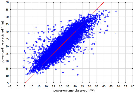
Figure 6.
Scatterplot of predictions of power-on-time versus real observations of ongoing process. The blue dots indicate the actual values, while the red line indicates the ideal predicted model.
As mentioned earlier, dual models proved to be the most effective. This means that a different model is used for the first heat in the sequence compared to the subsequent ones. Additionally, another model is required for predicting the time when the departure moment cannot be determined, which occurs when there is a casting on the LMS that is third in line to be casted (i.e., before it, two more heats will be casted on the CC). Therefore, the implementation of models in the system required the development of model-triggering mechanisms, specifically ones triggering the appropriate model at various stages of the smelting process:
- For the first heats in the sequence (H1), the ANN-v6-H1 model is activated.
- For subsequent heats in the sequence, the ANN-v6-H3 model is activated.
- If the heat is not the first (H3), but during its processing in CC there is still a preceding heat (where the difference in HeatNumber is greater than 1, indicating that the preceding heat has not yet started casting directly before the current one, and hence, the departure time from LMS is not known), then the ANN-v5 model is activated, which does not require a time input. This model will switch to ANN-v6-H3 when the second-to-last heat arrives at CC, and the predicted departure time can be obtained from LMS monitoring.
Activating these models during the processing of individual heats allows for increased momentary accuracy of the models. However, it complicates the global comparison of their accuracy. Therefore, the global assessment of the system relies not only on the accuracy of predicting power-on-time, but also on the system’s ability to forecast the correct temperature during operation, as well as the degree of actual overheating compared to what is predicted by the system in interaction with all predictive models.
5. Conclusions
In summary, in terms of modeling, the described system consists of (1) optimization models for sequencing heats based on Ant Colony Optimization (ACO) algorithms, (2) prediction models for power-on time using neural networks, and (3) computational models calculating the optimal departure time from the LMS based on the predicted overheating of the main ladle. The presented manuscript primarily addresses issues related to process modeling rather than implementation or deployment aspects. The use of machine learning models has enhanced the efficiency and quality of processes. The quality of the models themselves was described in previous sections. Optimization of planning has reduced the time required to execute sequencing plans to a few seconds, also integrating the order indexing and processing of orders into production orders, as well as automating the scheduling of rolling and steelmaking campaigns, and the algorithm matched the production plan by more than 95%. Additionally, the power-on-time prediction models allowed for the estimation of the main ladle heating time with 97% accuracy (MAE ~ 3%), which in turn led to very precise production control and consequently reduced overheating.
Tests of the system were performed using the current production. However, to avoid non-routine cases, the focus was on 300 heats covering steel grades that were most frequently encountered during the system’s training. It is obvious that, as new data and instructions come in, the system will require updates and further training. Based on the conducted analyses, the casting temperature was significantly lowered for each of the analyzed grades. Based on the evaluation of billets and noting the technical aspects of the equipment, together with experts, the optimal level was determined to be 25–35 °C both in terms of billet quality and equipment safety. The average drop in superheat values for the selected grades ranged from 7–12 °C. It is particularly satisfying that the greatest difference in the drop in superheat values was observed for the most crucial grades.
Author Contributions
Conceptualization, Ł.R. and K.R.; data curation, A.O., K.B., M.P. (Monika Pernach), M.P. (Michał Piwowarczyk) and S.K.; formal analysis, K.R., P.H. and F.H.; funding acquisition, Ł.R. and M.P. (Michał Piwowarczyk); investigation, K.R., Ł.R. and P.H.; methodology, K.R., Ł.R., S.K. and M.P. (Michał Piwowarczyk); project administration, Ł.R.; supervision, Ł.R., M.P. (Michał Piwowarczyk) and S.K.; validation, Ł.R., M.P. (Michał Piwowarczyk) and S.K.; writing—original draft, K.R., Ł.R., F.H. and M.P. (Michał Piwowarczyk); writing—review and editing, K.R., Ł.R. and M.P. (Michał Piwowarczyk). All authors have read and agreed to the published version of the manuscript.
Funding
This research was funded by financial support from the National Centre for Research and Development: Intelligent Development Operational Program: POIR.01.01.01-00-0996/19.
Data Availability Statement
Data are available on request due to legal restrictions.
Conflicts of Interest
Michał Piwowarczyk and Sebastian Kalinowski are employed by the CMC Poland Sp. z o.o. The authors declare that the research was conducted in the absence of any commercial or financial relationships that could be construed as potential conflicts of interest. Furthermore, the funders had no role in the design of the study; in the collection, analyses, or interpretation of data; in the writing of the manuscript; or in the decision to publish the results.
References
- Hay, T.; Visuri, V.-V.; Aula, M.; Echterhof, T. A Review of Mathematical Process Models for the Electric Arc Furnace Process, 2020. Steel Res. Int. 2020, 3, 2000395. [Google Scholar] [CrossRef]
- You, D.; Michelic, S.C.; Bernhard, C. Modeling of Ladle Refining Process Considering Mixing and Chemical Reaction. Steel Res. Int. 2020, 91, 2000045. [Google Scholar] [CrossRef]
- Zappulla, M.L.S.; Cho, S.-M.; Koric, S.; Lee, H.-J.; Kim, S.H.; Thomas, B.G. Multiphysics modeling of continuous casting of stainless steel. J. Mater. Process. Technol. 2020, 278, 116469. [Google Scholar]
- Santos, M.F.; Moreira, M.H.; Campos, M.G.G.; Pelissari, P.I.B.G.B.; Angélico, R.A.; Sako, E.Y.; Sinnema, S.; Pandolfelli, V.C. Enhanced numerical tool to evaluate steel ladle thermal losses. Ceram. Int. 2018, 44, 12831–12840. [Google Scholar]
- Logar, V.; Škrjanc, I. The Influence of Electric-Arc-Furnace Input Feeds on its Electrical Energy Consumption. J. Sustain. Metall. 2021, 7, 1013–1026. [Google Scholar] [CrossRef]
- Carlsson, L.S.; Samuelsson, P.B.; Jönsson, P.G. Using Statistical Modeling to Predict the Electrical Energy Consumption of an Electric Arc Furnace Producing Stainless Steel. Metals 2020, 10, 36. [Google Scholar] [CrossRef]
- Andonovski, G.; Tomažič, S. Comparison of data-based models for prediction and optimization of energy consumption in electric arc furnace (EAF). IFAC-PapersOnLine 2022, 55, 373–378. [Google Scholar] [CrossRef]
- Tomažič, S.; Andonovski, G.; Škrjanc, I.; Logar, V. Data-Driven Modelling and Optimization of Energy Consumption in EAF. Metals 2022, 12, 816. [Google Scholar] [CrossRef]
- Chen, C.; Liu, Y.; Kumar, M.; Qin, J. Energy Consumption Modelling Using Deep Learning Technique—A Case Study of EAF. Procedia CIRP 2018, 72, 1063–1068. [Google Scholar] [CrossRef]
- Carlsson, L.S.; Samuelsson, P.B.; Jönsson, P.G. Interpretable Machine Learning—Tools to Interpret the Predictions of a Machine Learning Model Predicting the Electrical Energy Consumption of an Electric Arc Furnace. Steel Res. 2020, 91, 2000053. [Google Scholar] [CrossRef]
- Torquato, M.F.; Martinez-Ayuso, G.; Fahmy, A.A.; Sienz, J. Multi-Objective Optimization of Electric Arc Furnace Using the Non-Dominated Sorting Genetic Algorithm II, (IEEE). IEEE Access 2021, 9, 149715–149731. [Google Scholar] [CrossRef]
- Safronov, A.; Ronkov, L.V.; Mal’ginov, A.N.; Ivanov, I.A.; Shchepkin, I.A.; Yashchenko, V.K.; Tokhtamyshev, A.N. Experience in Developing Digital Twins Of Melting Processes in EAF for Solving Technological Problems of Producing a Semi-Finished Product with Required Quality Characteristics. Metallurgist 2022, 65, 1299–1310. [Google Scholar] [CrossRef]
- Monostori, L. Cyber-physical production systems: Roots, expectations and R&D challenges. Procedia CIRP 2014, 17, 9–13. [Google Scholar]
- Bagheri, B.; Yang, S.; Kao, H.A.; Lee, J. Cyber-physical systems architecture for self-aware machines in industry 4.0 environment. IFAC-PapersOnLine 2015, 28, 1622–1627. [Google Scholar]
- Lins, T.; Oliveira, R.A.R. Cyber-physical production systems retrofitting in context of industry 4.0. Comput. Ind. Eng. 2019, 139, 106193. [Google Scholar]
- Hajder, P.; Opaliński, A.; Pernach, M.; Sztangret, Ł.; Regulski, K.; Bzowski, K.; Piwowarczyk, M.; Rauch, Ł. Cyber-physical System Supporting the Production Technology of Steel Mill Products Based on Ladle Furnace Tracking and Sensor Networks. In Computational Science–ICCS; Lecture Notes in Computer Science; Springer: Cham, Switzerland, 2023; Volume 14077. [Google Scholar] [CrossRef]
- Sztangret, Ł.; Regulski, K.; Pernach, M.; Rauch, Ł. Prediction of Temperature of Liquid Steel in Ladle Using Machine Learning Techniques. Coatings 2023, 13, 1504. [Google Scholar] [CrossRef]
- Tan, W.; Khoshnevis, B. Integration of process planning and scheduling—A review. J. Intell. Manuf. 2000, 11, 51–63. [Google Scholar] [CrossRef]
- Dorigo, M.; Stützle, T. Ant Colony Optimization; MIT Press: Cambridge, MA, USA, 2004. [Google Scholar]
- Eiben, A.E.; Smith, J.E. Introduction to Evolutionary Computing; Springer: Berlin/Heidelberg, Germany, 2015. [Google Scholar]
- Maravelias, C.T.; Sung, C. Integration of production planning and scheduling: Overview, challenges and opportunities. Comput. Chem. Eng. 2009, 33, 1919–1930. [Google Scholar] [CrossRef]
- Zhong, R.Y.; Huang, G.Q.; Lan, S.; Dai, Q.Y.; Zhang, T.; Xu, C. A two-level advanced production planning and scheduling model for RFID-enabled ubiquitous manufacturing. Adv. Eng. Inform. 2015, 29, 799–812. [Google Scholar] [CrossRef]
- Guzman, E.; Andres, B.; Poler, R. Models and algorithms for production planning, scheduling and sequencing problems: A holistic framework and a systematic review. J. Ind. Inf. Integr. 2022, 27, 100287. [Google Scholar] [CrossRef]
- Gumienny, G.; Kacprzyk, B.; Mrzygłód, B.; Regulski, K. Data-Driven Model Selection for Compacted Graphite Iron Microstructure Prediction. Coatings 2022, 12, 1676. [Google Scholar] [CrossRef]
- Breinman, L.; Friedman, J.H.; Olshen, R.A.; Stone, C.J. Classification and Regression Trees; Chapman and Hall: London, UK, 1993. [Google Scholar]
- Dučić, N.; Jovičić, A.; Manasijević, S.; Radiša, R.; Ćojbašić, Z.; Savković, B. Application of machine learning in the control of metal melting production process. Appl. Sci. 2020, 10, 6048. [Google Scholar] [CrossRef]
- Cardoso, W.; di Felice, R.; Baptista, R.C. Artificial Neural Network for Predicting Silicon Content in the Hot Metal Produced in a Blast Furnace Fueled by Metallurgical Coke. Mater. Res. 2020, 25, e20210439. [Google Scholar] [CrossRef]
- Tadeusiewicz, R. Neural Networks in Mining Sciences—General Overview And Some Representative Examples. Arch. Min. Sci. 2015, 60, 971–984. [Google Scholar] [CrossRef]
- Joshi, A.V. Machine Learning and Artificial Intelligence; Springer Nature Switzerland AG: Cham, Switzerland, 2020. [Google Scholar]
- Noh, S.-H. Analysis of Gradient Vanishing of RNNs and Performance Comparison. Information 2021, 12, 442. [Google Scholar] [CrossRef]


Disclaimer/Publisher’s Note: The statements, opinions and data contained in all publications are solely those of the individual author(s) and contributor(s) and not of MDPI and/or the editor(s). MDPI and/or the editor(s) disclaim responsibility for any injury to people or property resulting from any ideas, methods, instructions or products referred to in the content. |
© 2024 by the authors. Licensee MDPI, Basel, Switzerland. This article is an open access article distributed under the terms and conditions of the Creative Commons Attribution (CC BY) license (https://creativecommons.org/licenses/by/4.0/).