Abstract
Dynamic fracture propagation significantly affects water flooding efficiency in tight oil reservoirs. This phenomenon, where moderate fracture openings can enhance water flooding volume and alleviate injection challenges, has been underexplored in current literature. Understanding dynamic fracture behavior poses a challenge due to the difficulty in characterizing them within traditional reservoir numerical simulators. In this study, we propose a numerical simulation method that integrates the KGD dynamic fracture model with a two-phase flow model. This approach enables detailed exploration of dynamic fracture evolution in reservoir scenarios featuring one injector and one production well. Our findings reveal that fractures extend from the water injection well to the oil production well, exhibiting rapid initial growth followed by a slower rate. Fluctuations in fracture tip pressure correspond to cycles of opening and closure. We observe that cumulative oil production increases more rapidly when injection pressure exceeds the fracture opening pressure. However, this growth rate diminishes beyond a certain threshold, highlighting the critical role of injection parameters in dynamic fracture efficacy. Optimal water flooding performance is achieved when injecting water slightly above the fracture opening pressure. Furthermore, we compare water cut curves generated by conventional commercial simulators with our fracture propagation model. Our model’s water cut curve aligns better with on-site data, indicating improved historical fitting accuracy. In conclusion, our study underscores the importance of dynamic fractures in enhancing water flooding efficiency in tight oil reservoirs and presents a robust numerical simulation framework for better understanding and management of reservoir dynamics.
1. Introduction
The development of tight oil reservoirs is currently a research hotspot, and tight oil is an important growth point for crude oil production. Improving the level of tight oil development is the top priority for increasing oil production [1,2,3,4,5,6,7,8]. Water injection in tight oil reservoirs is a challenging task, as excessive water injection leads to the water cut increasing quickly, while insufficient water injection results in low formation energy and less oil production. An important reason for the water cut increasing rapidly is the fractures propagate caused by water injection. As the water injection continues, the pore pressure increases and the closed fractures open gradually, leading to injected water flowing along open fractures, which results in early watered-out producers and declining yield. Therefore, understanding the fracture extend rules and applying it to the field is challenging, with many unknowns waiting to be explored.
Several scholars have conducted relevant research on dynamic fractures. Most research on dynamic fracture has focused on modeling hydraulic fracturing processes [9,10,11] to simulate fluid injection-induced fracture activation, damage growth, seismicity occurrence, and connectivity change in naturally fractured rocks through the finite element method [12]. However, the target of those studies is to obtain the permeability damage, the fracture development, and the geomechanical effects during fracture propagation. This model only considers the situation of single-phase flow and does not discuss the fracture changes under two-phase flow conditions. Meanwhile, two classical fracture models were presented to characterize fracturing, including KGD models [13,14] and PKN models [15], which could characterize the fracture propagation. Nevertheless, the models were only applied to single-phase fluid flow and are simplified analytical models. Yang Wang et al. developed a comprehensive method to recognize the fracture opening, provided a dedicated methodology for the fracture closure process, and built a well-testing model that characterizes closures of single and multiple fractures that can help obtain dynamic fracture parameters [16]. Zhang and Emami-Meybodi built a flowback model of rate transient analysis that takes the two-phase flow and characterizes the flow stage of the dynamic fractures [17]. The model was applied in the field and the results were highly consistent with the filed results. Lei Zhengdong et al. developed a dynamic discrete fracture model (DDFM) to characterize dynamic fracture and simulate complicated multiphase flow in a fractured tight reservoir [18,19]. This model could simulate the deformation of dynamic fractures based on geomechanics and update the unstructured grids, which resulted in an increase in pre-processing workload and longer numerical simulation computation. Yang et al. presented a model that characterizes the heterogeneity caused by dynamic fractures during the water injection process [20]. The model updates the dynamic embedded discrete fracture model (DEDFM) through grid preprocessing at every time step, which results in high computation. It is difficult to solve when many fractures exist in the model.
Therefore, this paper aims to develop an effective and efficient model of dynamic fracture induced by water injection, which can more finely characterize dynamic fracture and decrease computational complexity. A method coupled with the KGD model and an oil–water two-phase flow model is first presented to establish a reservoir numerical model with dynamic fracture. We use this model to explore the change rule of dynamic fracture during water injection and apply it to the field, fitting it well with the field data, which has important guiding significance for the study of water injection in fractured reservoirs.
2. Methodology
In this section, we established an oil–water two-phase flow model considering fracture propagation. Firstly, we obtained the block center finite volume discretization format of the flow control equation, then we built the fracture propagation model. Finally, we coupled the two models for calculation by modifying the conductivity.
2.1. Oil–Water Two-Phase Flow Mathematical Model
The embedded discrete fracture model (EDFM) only requires a structured matrix grid, which has lower requirements compared to the conventional discrete fracture model (DFM). For the EDFM, Cartesian coordinates are generally used to facilitate the calculation of parameters for each grid surface, and the finite volume method (FVM) can be implemented well in this grid system. Therefore, we chose the FVM as the numerical method for the discrete seepage control equation in the EDFM.
The continuity equation of oil components is [21]:
where km is the matrix permeability, kro(cp) is the relative permeability of the oil phase, Bo is the crude oil volume coefficient, ρosi is the crude oil density under standard conditions, D is the altitude, ϕ is the porosity, So is the oil saturation, qos is the volumetric flow rate, and δ is the Dirichlet function.
We converted this equation to an implicit format; the continuity equation of oil components can be obtained using a finite volume discretization scheme at the center of the block.
where Tij is the grid conductivity between two grids, λo,ij is the oil phase fluidity between adjacent grids, μo,ij is the arithmetic mean of the viscosity values in adjacent grids, Bo,ij is the arithmetic mean of the crude oil volume coefficient in adjacent grids, and ∆Vi is the grid volume of the ith grid.
where μo,i and μo,i are the viscosity values of the ith and jth blocks, and Bo,i and Bo,j are the viscosity values of the ith and jth blocks.
Similarly, a block-centered finite volume discretization scheme can be obtained for the continuity equation of water components.
2.2. Fracture Propagation Model Induced by Water Injection
The formation mechanism of dynamic fracture is complex, and the fracture morphology continuously changes during the fracture propagation. We introduced the KGD model to characterize the fracture propagation; the fracture height, length, and width are dynamically changing during the water injection. The study is based on following assumptions:
- (1)
- The height, length, and width are given by the KGD model, which is intended to compute fracture geometry under given pressures and stresses. The fracture is two-dimensional and the height is fixed.
- (2)
- The EDFM fractures pass through several matrix grids and have different widths along the fracture from the well bore to the fracture tip, and the pressures of different fracture segments are various.
- (3)
- Fluid in the fracture is considered to be an oil–water two-phase flow and the effect of capillary pressure is also considered.
- (4)
- The influence of thermal stresses induced by cold water injection is neglected in this model. Particle plugging of is also not considered here.
- (5)
- The fracture direction is consistent with the grid direction.
2.2.1. Fracture Opening
When fracture pressure increases above or decreases below a certain value, the fracture will open/close. The fracture opening/closing pressure in two-dimensional space is:
where Pf is the fracture opening/closing pressure, σH is the maximum principal stress, σh is the minimum principal stress, θ1 is the angle between the fracture direction and minimum principal stress, and θ2 is the angle between the fracture direction and maximum principal stress.
2.2.2. Stress Change
The equation of maximum/minimum principal stress is [22]
where τHi is the initial maximum principal stress, τhi is the initial minimum principal stress, and Ape is the pore-elastic constant of the rock [23]:
where αB is the Biot constant, and γ is the Poisson’s ratio.
2.2.3. Fracture Length
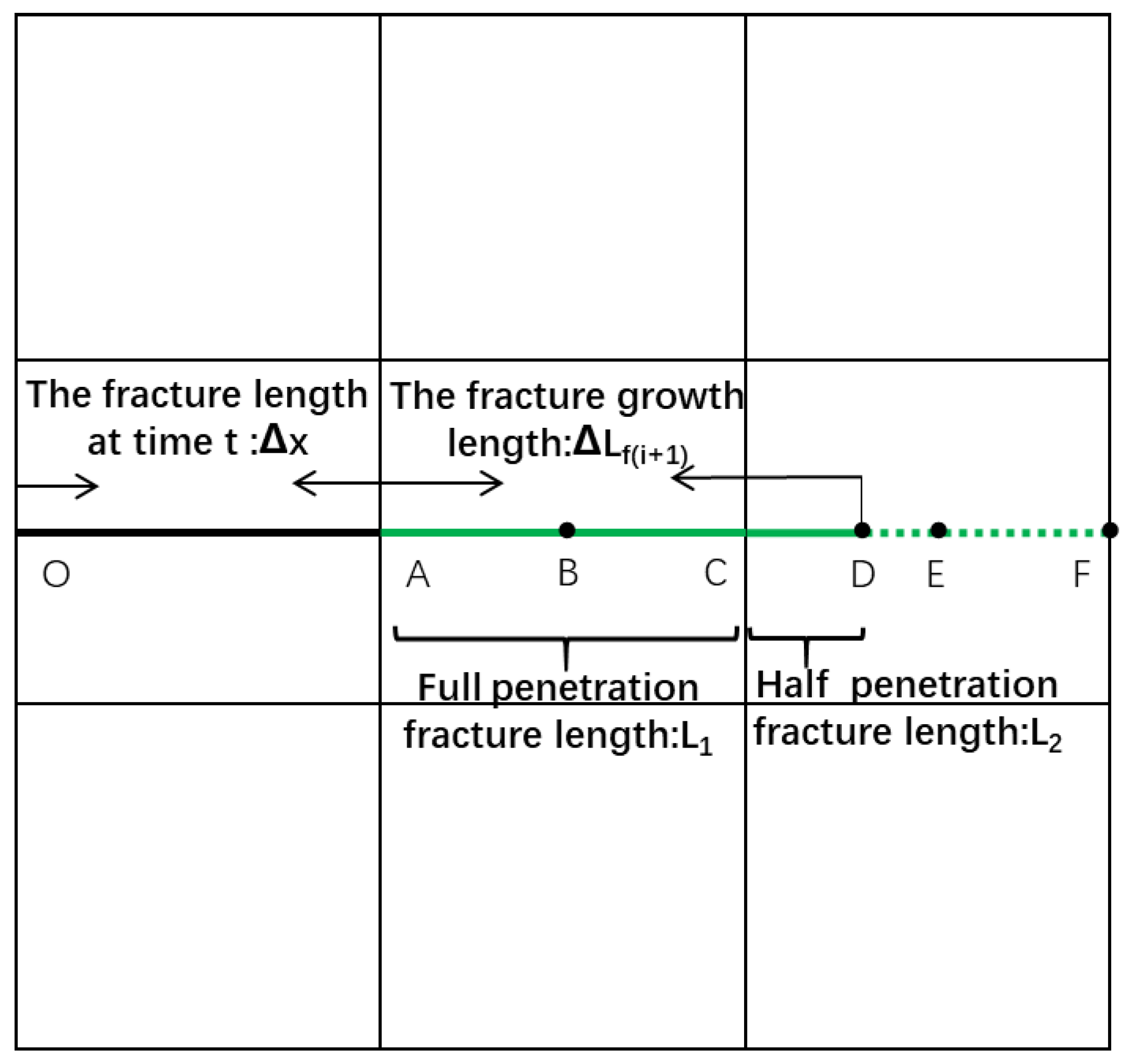
The length of dynamic fracture is calculated based on the KGD model. At the time point from t to (t + ∆t), we try to search grid pressures of each fracture grid and confirm the ith fracture grid is greater than the opening pressure and that the (i + 1)th fracture grid pressure is lower than the fracture opening pressure. The fracture point is located between the (i + 1)th fracture grids, which is between B and E especially, as shown in Figure 1. In order to determine the location of fracture point accurately, the pressures of the two fracture grids are linearized, and the pressures at points C and E are respectively taken as the grid pressure Pf(i) and Pf(i+1). The equation is as follows:
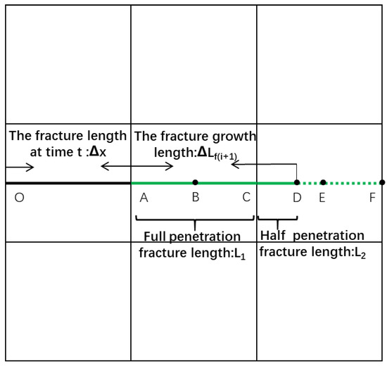
Figure 1.
Fracture propagation length at time t + ∆t, which includes the fracture length of the fully and partially penetrated grid block.
As shown in Figure 1, point O is the starting point of fracture opening, points A, C, and F are the intersection points of the matrix and the fracture grid, points B and E are the midpoints of the matrix grid.The direction of fracture propagation is determined with the original fracture length Lf(i). In order to determine the incremental fracture length AD = ∆Lf(i+1) at any given time step from t to t + ∆t, the newly increased fracture segment is divided into a fully penetrated section AC and a partially penetrated section CD. For the first part, the length of every fracture segment is
where M is the number of open fractures, and ∆x is the matrix grid length in the x direction.
For the second part, the length of the fracture in the partially penetrated reservoir block is computed based on the pressure distribution of adjacent fracture grids. Specifically, the pressure of point C is Pf(i+1), which exceeds the fracture opening fracture, and the pressure of point E is Pf(i+1), which is less than the fracture opening pressure. It can be confirmed that the fracture tip is located between the midpoints of the two fracture grids (between C and E). Hence, we obtain the position of the fracture tip by linearizing the pressure, and the length of the fracture partially penetrating the matrix grid is
where ∆x is the matrix length in the x direction.
The fracture length in this time step is
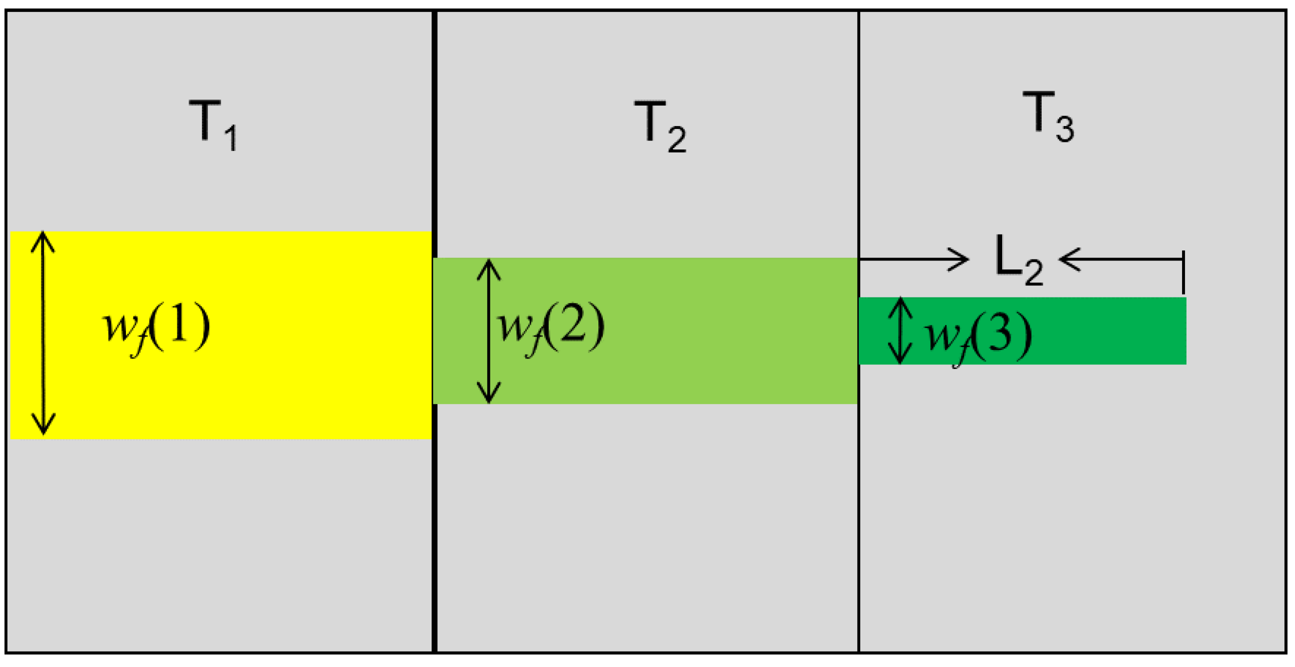
2.2.4. Fracture Width
The fracture width varies (Figure 2), and we calculate the width based on the GDK model [13,14]. The relationship between the fracture width and fracture length is
where E is the Young’s modulus, and Pi is the pressure of the ith fracture grid.
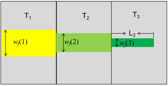
Figure 2.
The different width of different fracture segments at time t + ∆t.
2.2.5. Fracture Permeability
The fracture width wf(i, t) is the ith fracture grid in time t, which can be calculated by Equation (16), and the fracture permeability can be calculated by using the Poiseuille equation. Therefore, the permeability of the fracture at a distance x from the fracture initiation point in the ith time step is [24]
where kf(x, 0) is the initial permeability when the fractures open, wf(x, 0) is the initial fracture width, and wf(x, t) is the fracture width for time t.
In order to characterize dynamic fracture, the embedded discrete fracture model (EDFM) is introduced. In this model, the conductivity between two adjacent matrix grids within same fracture is
where Ti and Tj are the ith and jth fracture grids, kf(i) and kf(j) are the permeability of the ith and jth matrix grids, wi and wj are the widths of the ith and jth fractures, and h is the fixed fracture height.
In order to improve the stability of the coupled model caused by the permeability contrast between fractures and matrix grids, we introduce a method that equals the fracture permeability to matrix permeability [25]. For the fracture grid fully penetrating the matrix grid, the equivalent matrix permeability is
where kx1 is the equivalent matrix permeability, kx is the permeability in the x direction, and ∆y is the matrix grid length in the y direction.
For the fracture grid partially penetrating the matrix grid, the equivalent matrix permeability is
2.3. Numerical Simulation Calculation Process
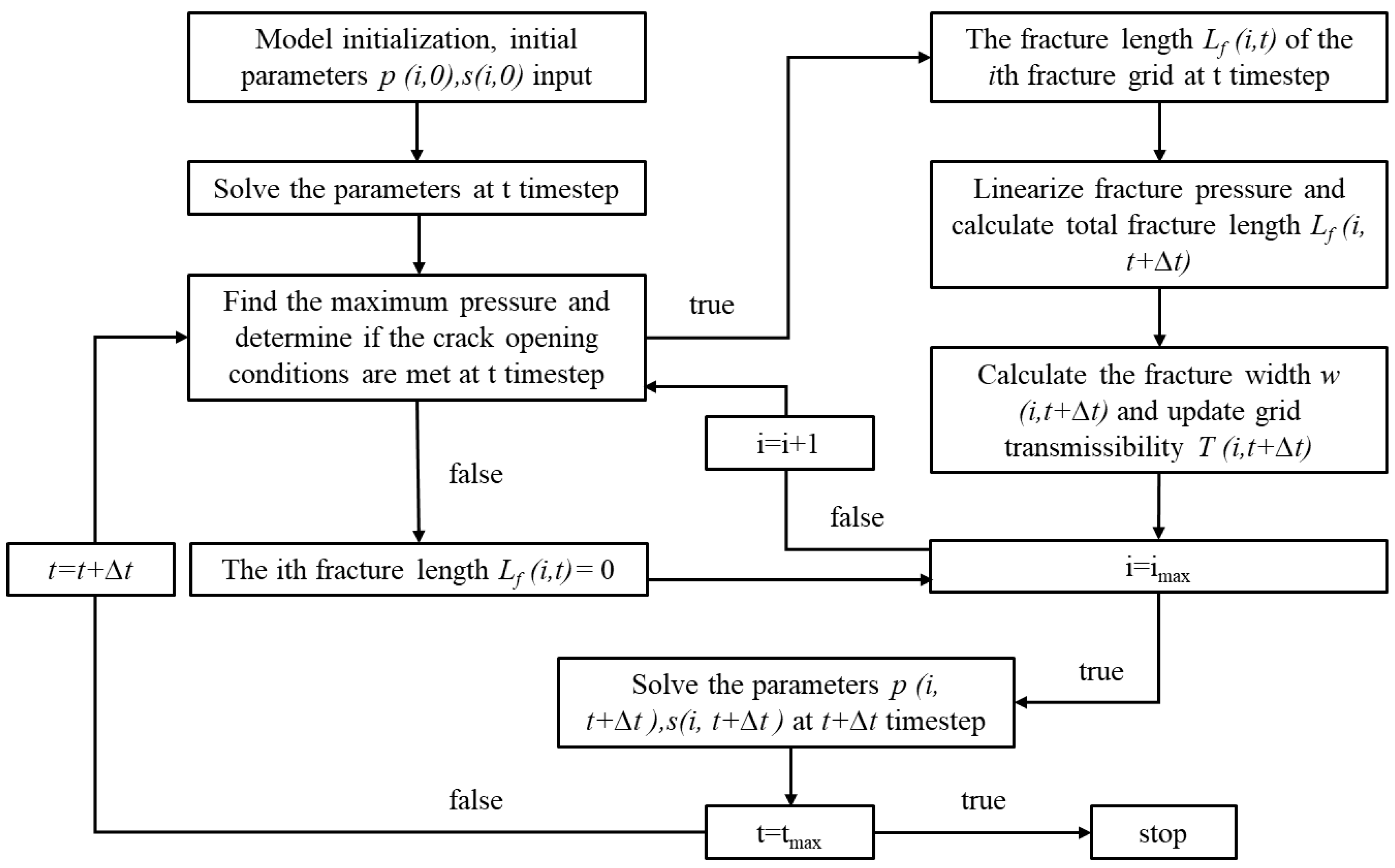
As the Figure 3 shows, a numerical model of an oil–water two-phase reservoir considering the dynamic fractures is established. The simulator couples the KGD fracture propagation model with the oil–water two-phase flow model, in which the change in grid conductivity is used to reflect the process of fracture opening and extension. By comparing the pressure of fracture grids, the simulation starts with a process to confirm the fracture state is open or closed. Then, the length of the fracture in the partially penetrated matrix can be obtained by linearizing the pressure value and confirming the fracture point, which helps obtain the widths of every fracture grid based on the KGD model. Next, the change in fracture conductivity is equivalently applied to the matrix grids where the fracture grids are located. Last, the updated reservoir properties are input into the simulator to solve the pressure values, water, oil saturation, and so on, which cause an interplay problem that must be solved. The specific calculation process is as follows:
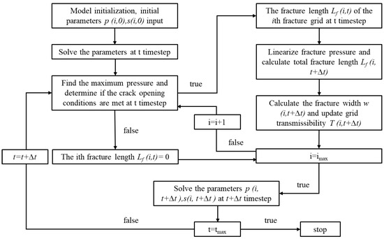
Figure 3.
Numerical simulation calculation flowchart of the fracture propagation model.
- (1)
- Confirm the fracture grid state at time t. At the initial moment, the initial grid pressure P(i,0) and saturation S(i,0) at t time are input, there are no fracture grids for which the pressure is greater than opening pressure, and all the fracture grids are closed. At time t, the pressures of all fractures is compared with the opening pressure to determine the opening fracture grids.
- (2)
- Confirm the fracture geometry at time t + ∆t. All the pressures of the fracture grids are compared with the opening pressure to confirm that the pressure Pf(i, t) of the ith fracture grid is greater than the fracture opening pressure, while the pressure Pf(i + 1, t) of the adjacent i + 1th fracture grid is lower than the fracture opening pressure, so the length of fracture fully penetrating the matrix grid can be calculated. Then, focus on the length of the fracture partially penetrating the matrix grid. In order to determine the position of the fracture tip, linearize the pressures between adjacent fracture grids along the fracture extension direction. The total fracture length is the sum of the fracture lengths of the two parts mentioned above. We can use the KGD model to calculate the width distribution with Equation (16).
- (3)
- Update the fracture conductivity of the fracture grids according to the fracture width distribution with Equation (17). The change in fracture conductivity is equivalent to the matrix grid where they are located based on Equations (21) and (22). Based on Formulas (18)–(20), modify the fracture grid conductivity Ti and Tj to achieve the goal of modifying the fracture conductivity.
- (4)
- Use the coupled model to perform reservoir numerical simulation and solve the pressures P(i, t + ∆t) and saturation S(i, t + ∆t) of every grid at time t + ∆t. Repeat steps (1), (2), and (3) until the end of the last time step.
To execute this algorithm, we utilized MATLAB Reservoir Simulation Toolbox (MRST) for code editing of the algorithm [26,27].
3. Results and Discussion
3.1. Model Verification
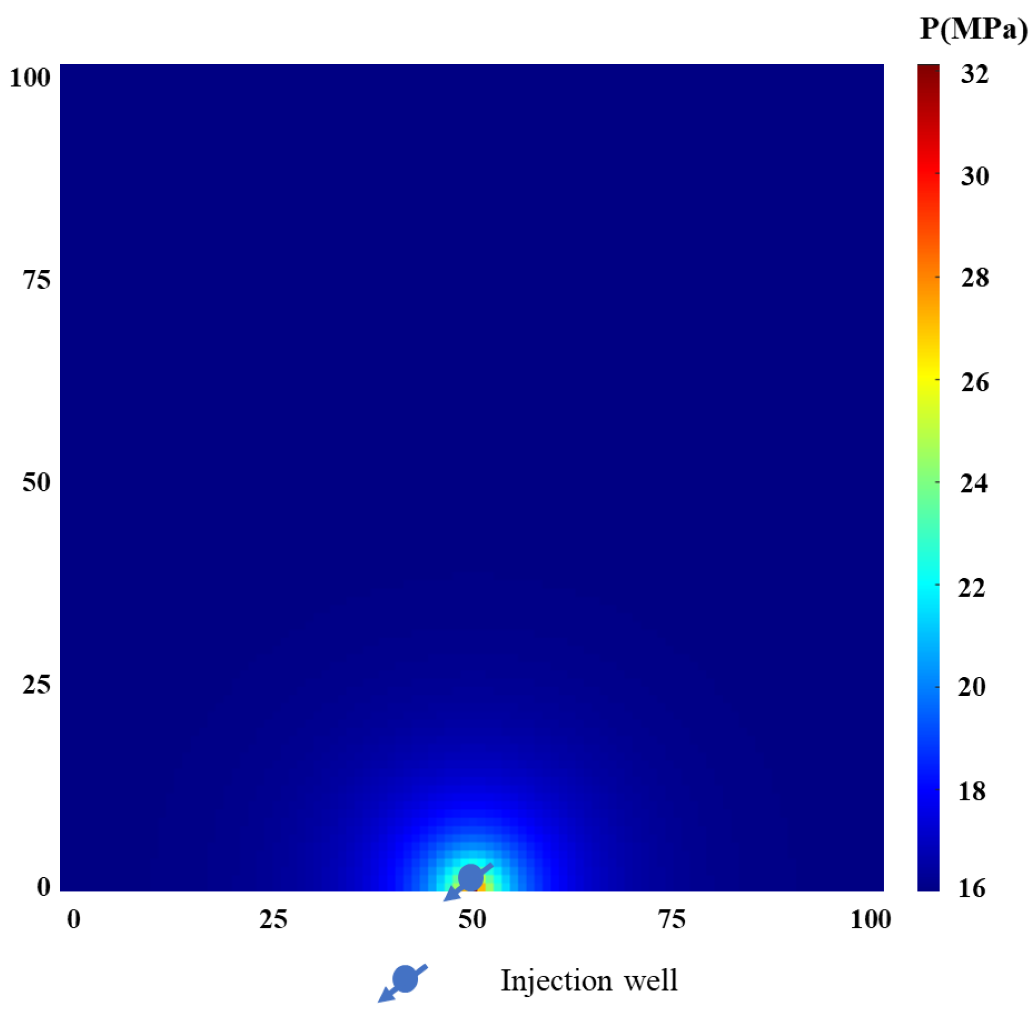
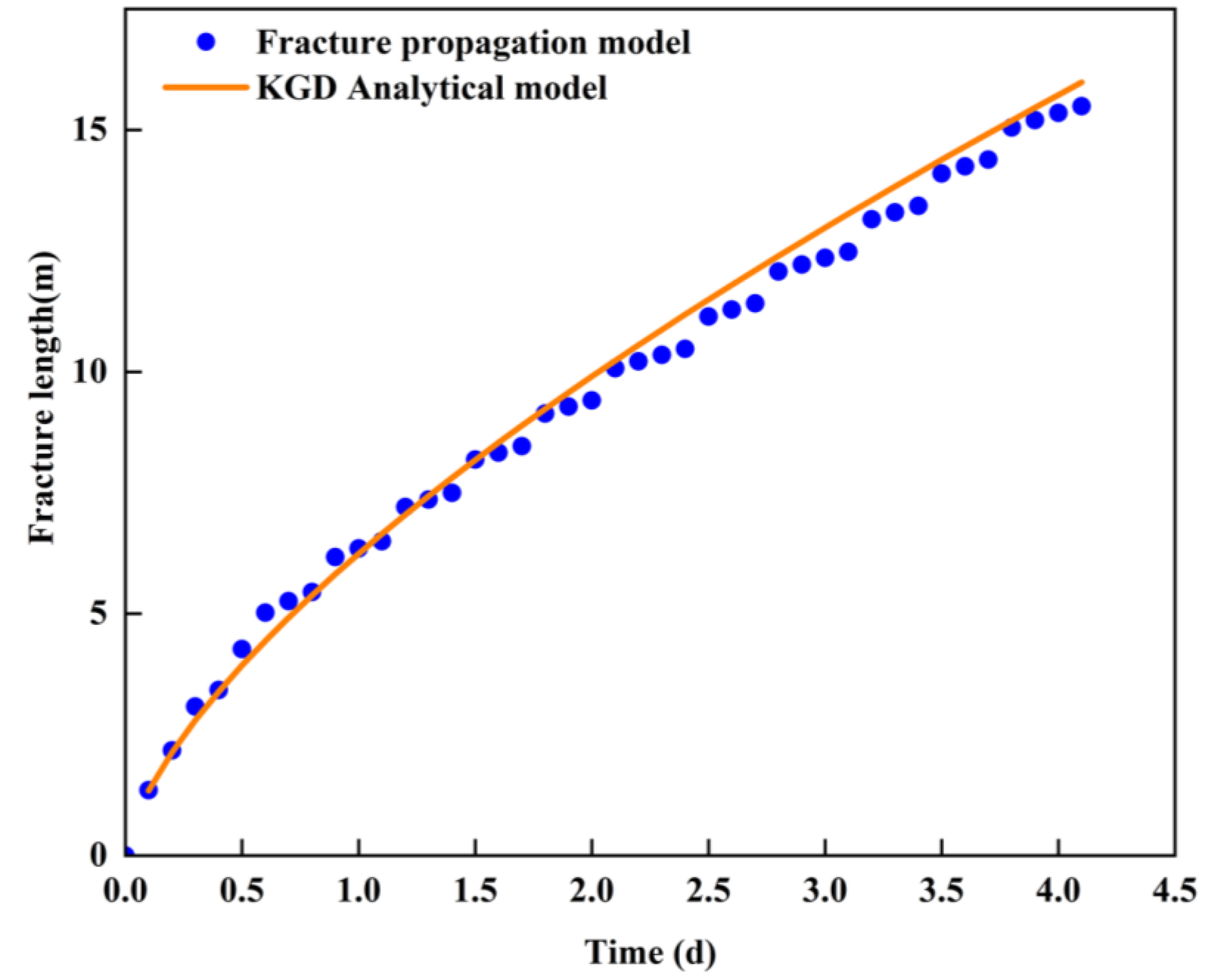
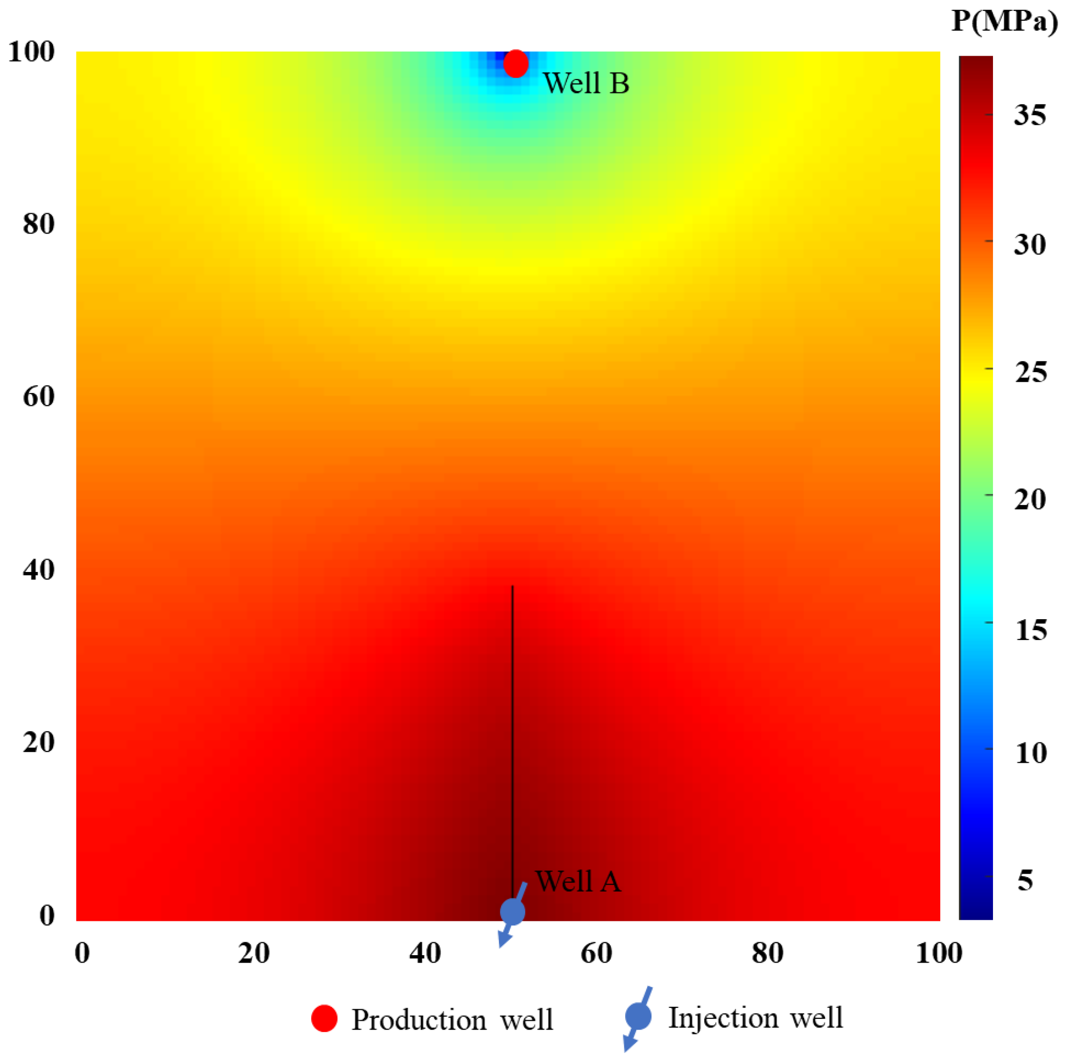
In order to demonstrate the reliability of the model, we carry out model validation and compare the fracture length change curves of the fracture propagation model and the KGD analytical model. The grid number is 101 × 101 × 1 and the main parameter is in Table 1. The injection well is located in the middle point of the lower boundary and the water injection rate is 3.5 m3/d (Figure 4). As Figure 5 shows, there may be slight differences between the fracture length of the fracture propagation model and the analytical solution of the KGD model, with the fracture length of the fracture propagation model undergoing a sudden change, which is due to the mesh division and numerical discretization in the fracture propagation model. However, the results show that the fitting effect is good and that the fracture propagation trend is consistent.

Table 1.
The main reservoir parameters of a typical case.
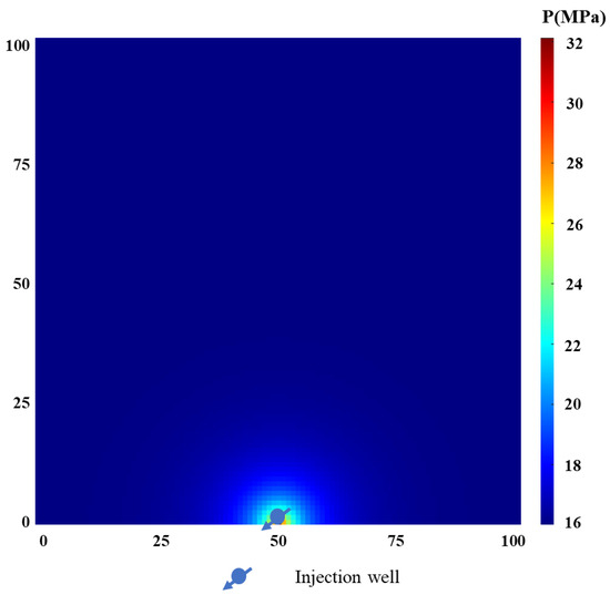
Figure 4.
The pressure distribution map of a single well water injection at the initial moment.
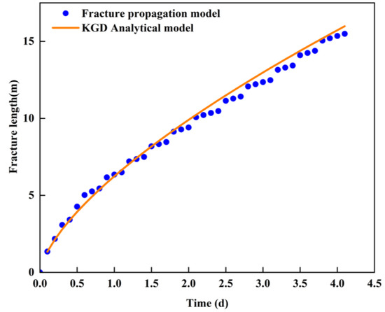
Figure 5.
The fracture length change curve of the fracture propagation model and the KGD analytical model.
3.2. The Fracture Propagation Law
A single well injection and a single well production model is established as a typical case to study the law of fracture propagation. The main parameters of the model are given in Table 1, including the reservoir dimension, permeability, porosity, rock compressibility, and so on. Water injection well A is in the middle of the bottom boundary, while the production well B is in the middle point of the top boundary (Figure 6). Well A injects water at a contrasting pressure of 39 MPa and well B produces a contrast pressure of 2 MPa. The simulation time is 400 days. It is also assumed that the fracture extension direction is along the y axis, which is the maximum stress direction.
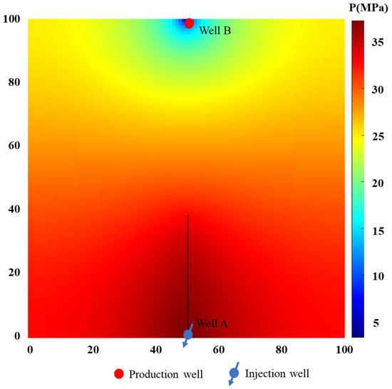
Figure 6.
Pressure distribution map and fracture propagation morphology during 400 days of water injection under one injection and one production mode.
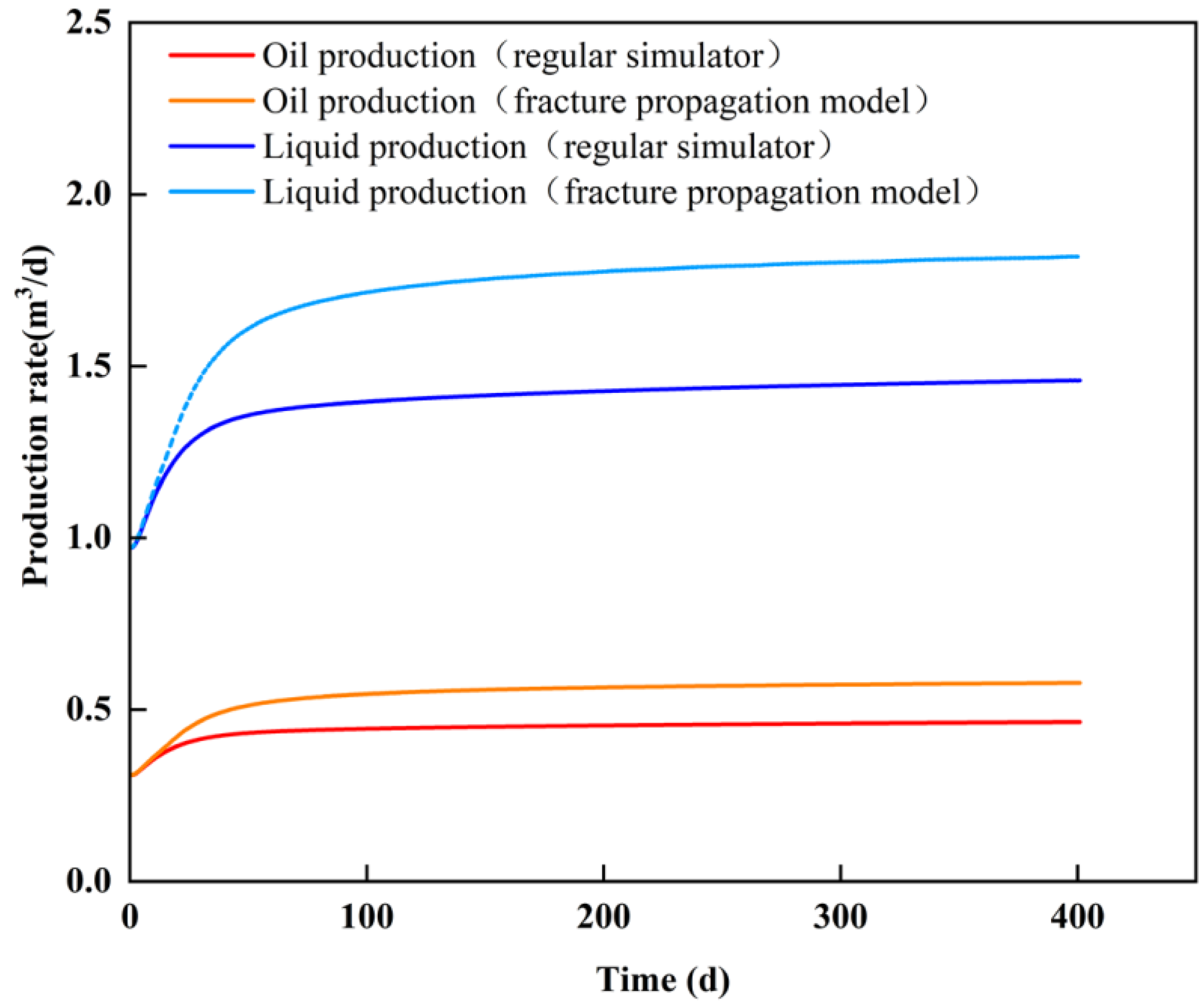
Figure 7 shows a comparison between our fracture propagation model and a regular numerical simulator simulation of the production curve after 400 days of water injection. It can be observed that the daily oil and liquid production under the fracture propagation model is higher than that under the regular simulator. Regular simulators cannot simulate the dynamic expansion of fractures, which can result in significant errors.
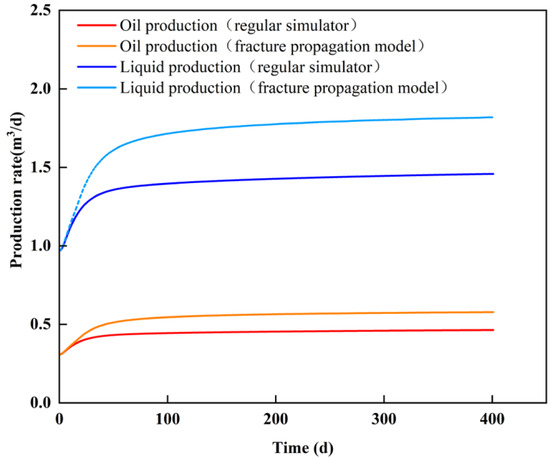
Figure 7.
The comparison of production between the regular simulator and the fracture propagation model.
Figure 8 is the oil saturation distribution map at a different time, which shows that injected water flows along the dynamic fracture and is different from the model without dynamic fracture. The oil–water front moves rapidly forward along the fracture at an early time and spreads on both sides of the fracture after the movement speed of the oil–water front becomes slow, which is caused by the slowing down of the fracture extension speed. The movement distance of the water front in the x direction is about 10 m, and the movement distance in the y direction is 45 m; the movement distance of the water front in the x direction is much shorter than the distance in the y direction. This is because the dynamic fractures become highly permeable flow channels and the oil–water front moves faster along the maximum stress direction [28]. This indicates that it is difficult for the injected water to flow along the minimum principal stress direction even if the production well in the x direction is closer to the injection well.
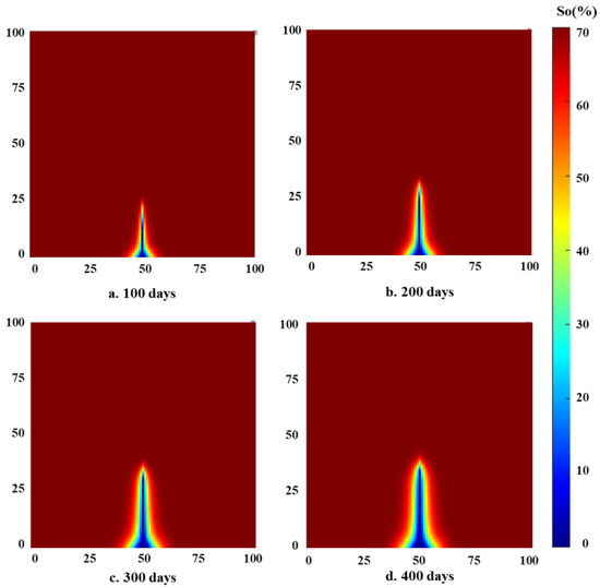
Figure 8.
The oil saturation distribution map at different times during water injection.
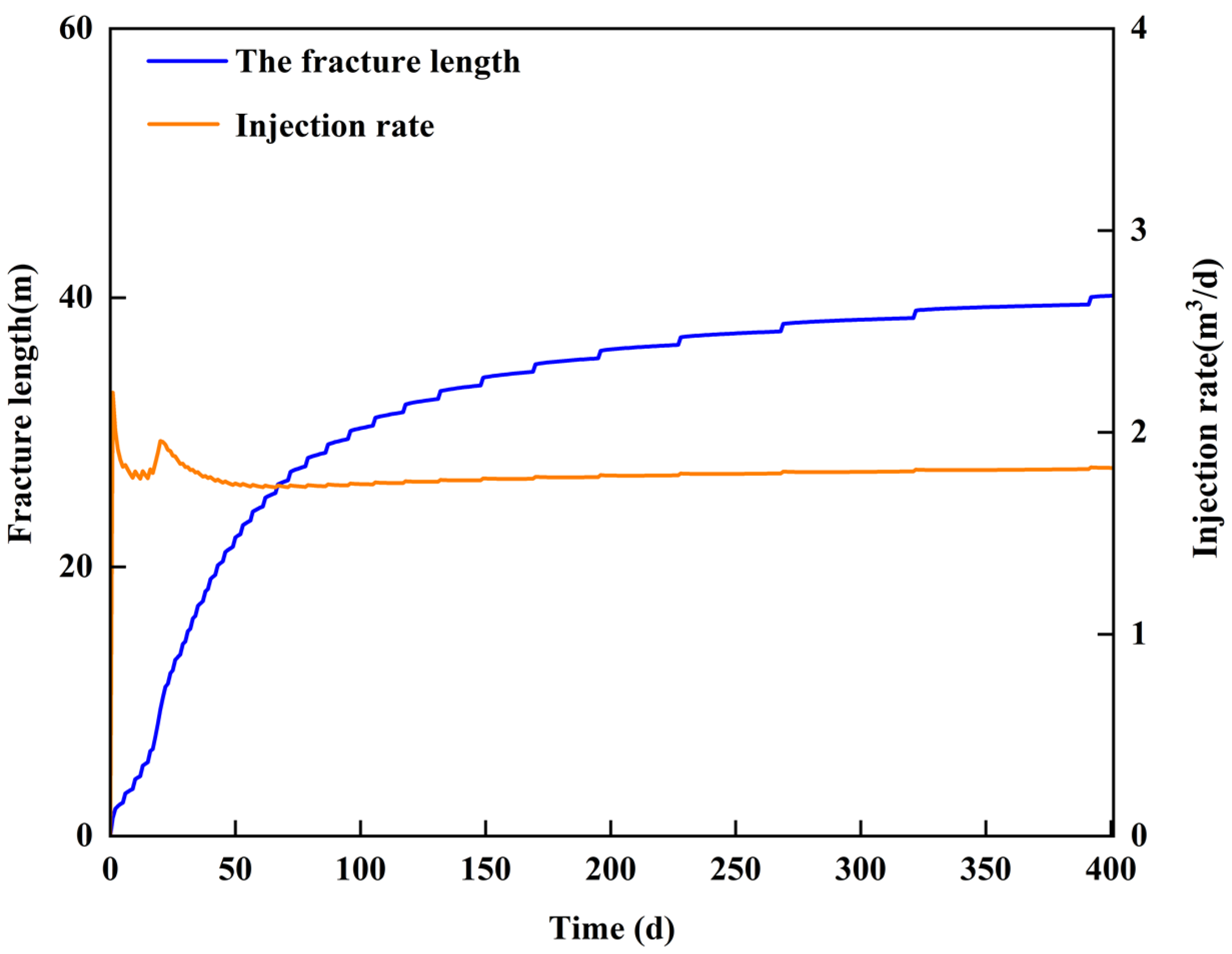
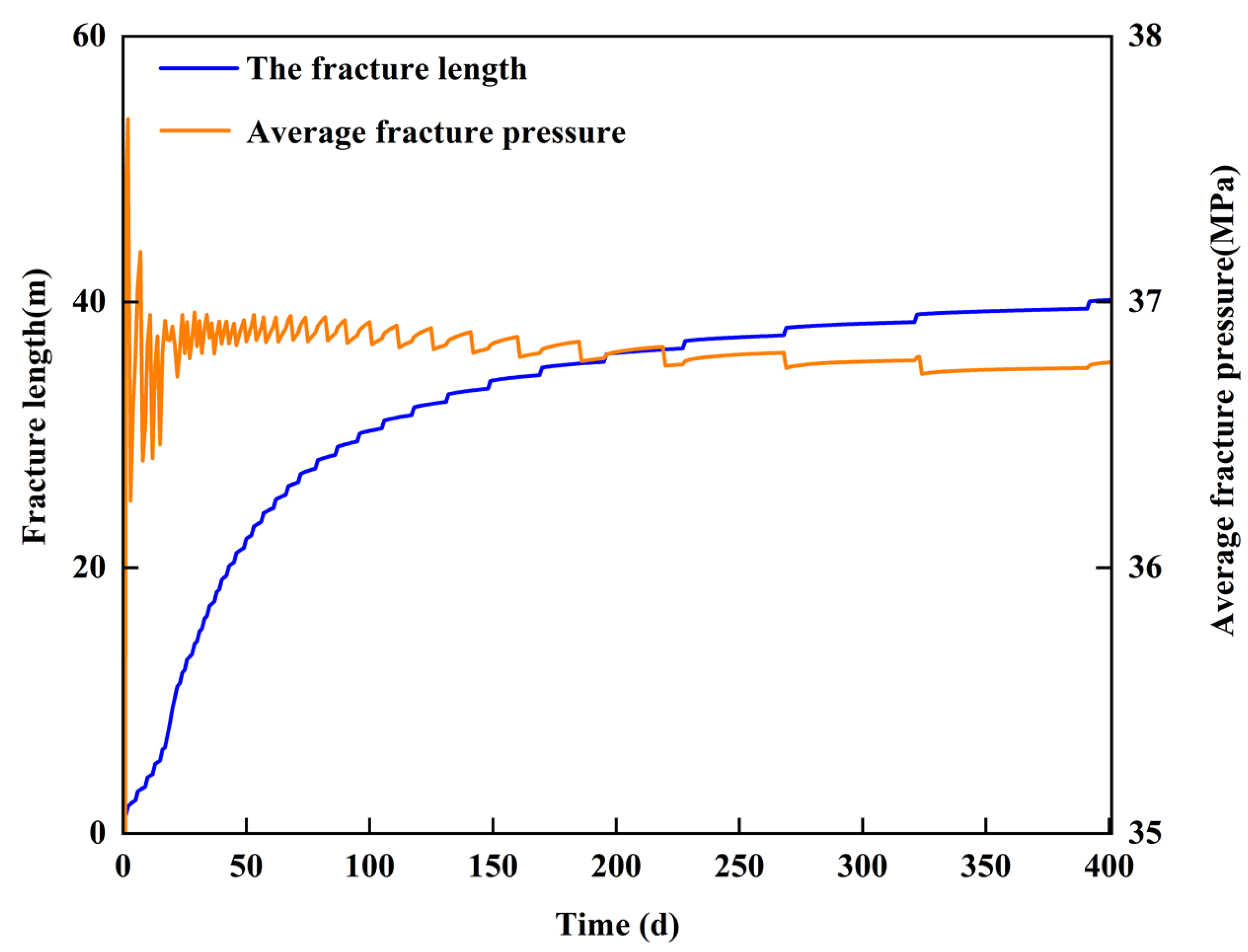
Figure 9 and Figure 10 shows that fracture length and injection rate change during water injection. The fracture length increases fast in the first 100 days, and then the growth rate decreases quickly. In the early stage, large quantities of fluid flow into the fracture, which causes a rapid increase in fracture pressure, and the fracture extends fast. The water injection rate falls off at the beginning because the volume of the opening fracture is too small to accommodate more injected water and the bottom pressure increases too fast. When the fracture extends to 9.2 m, the fracture point pressure decreases rapidly, which leads to a sudden increase in the water injection rate. The reason is that accelerated propagation of the fracture tip leads to a pressure deficit at the tip and a sudden expansion of the production pressure difference, which leads to the sudden increase in the water injection rate. The fracture point pressure follows a distinctive pattern of “pressure increase—fracturing—pressure decrease” [29].
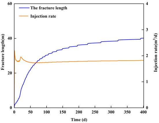
Figure 9.
The fracture length and injection rate during water injection.

Figure 10.
The fracture length and fracture point pressure vs. time.
The fracture point pressure curve exhibits a jagged feature; a decrease in the curve indicates the opening of a new fracture segment with a brief pressure deficit at the tip, and an increase in the curve indicates the energy is accumulated at the tip. The new fracture segment opens along with the fluctuation in pressure at the fracture tip. The increasing segment of the pressure curve at the fracture tip becomes longer, which indicates that the time interval for holding pressure at the fracture tip becomes longer and the fracture propagation speed is slower. The key reason is that the fracture tip farther away from the wellhead has a greater pressure difference with the matrix around the fracture tip, and the fluid in the fracture has faster leakage.
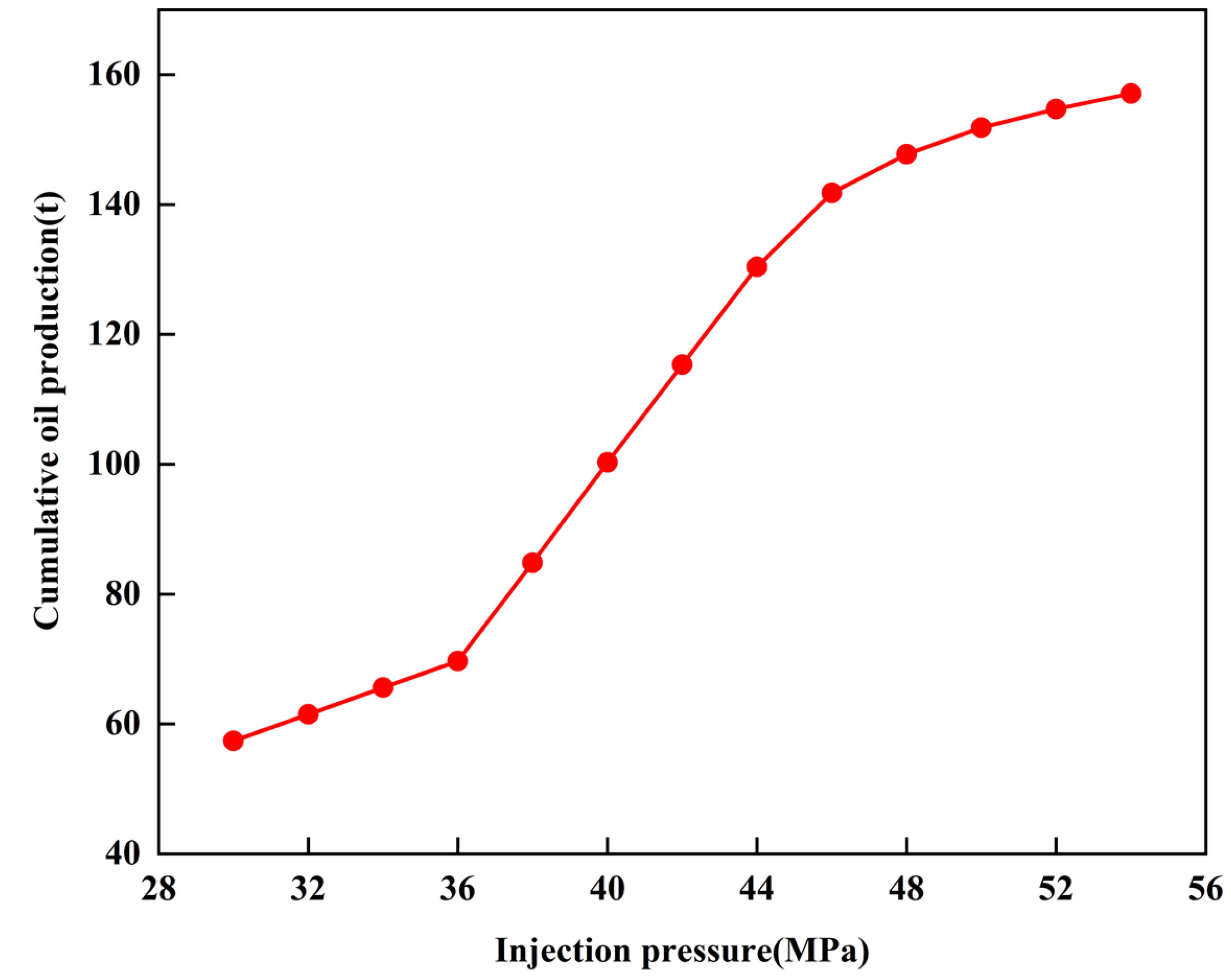
Figure 11 shows the cumulative oil production vs. injection pressure. The cumulative oil production increases with the injection pressure, the growth rate is low when the injection pressure is lower than 36 MPa or greater than 46 MPa, and the cumulative oil production increase quickly when the injection pressure increases from 36 MPa to 46 MPa. When the injection pressure is lower than the critical opening pressure (33.4 MPa), the fracture is closed, which leads to low water injectivity, and the cumulative oil increases slowly with the injection pressure increase. When the injection pressure exceeds the critical opening pressure, the dynamic fracture opens, the water injectivity of the injector well increases, and the oil production grows fast. When the injection pressure exceeds 46 MPa, the oil production growth rate, excessive water injection leads to excessive expansion of the fracture [30]. Although a large amount of water injection significantly increases the water injectivity, the injected water flows along the opening fracture, which results in a low increase in oil production.
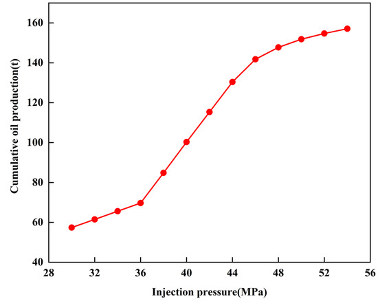
Figure 11.
The cumulative oil productions under different injection pressures.
3.3. Field Application
In this section, a field case is studied. The ultra-low reservoir is in northwest China and an inverted nine-spot rhombus well pattern is adopted. The maximum principal stress is in the x direction, which is parallel to the fracture extension direction. As shown in Figure 11, there is one injection well in the middle and eight production wells around the injection well. The initial model properties are unchanged until the fracture opens. The main injection-production parameters are shown in Table 2.
Table 2.
The main reservoir parameters of a typical case.
As Figure 12 shows, well I1 injects water for 8 years, and the water cut of wells P1 and P5 quickly climbs from 20% to 80% in the first 4 years. Figure 13 shows that the water cut curve of the fracture propagation model using the EDFM is in good agreement with the actual curve, while the water cut curve simulated by Navigator without a dynamic fracture has a large deviation compared with the actual curve. These two wells were converted to a water injection well. The main reason is that the dynamic fracture model considers the variation in fracture permeability and the high permeability channels between the injection and production wells lead to premature water breakthrough in the production wells. However, the regular model without considering fracture permeability changes under Navigator cannot characterize the high permeability channels.
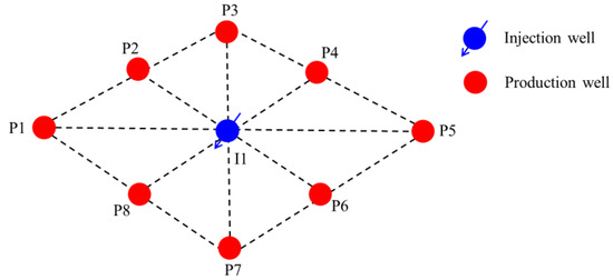
Figure 12.
Schematic diagram of diamond-shaped reverse nine-point well network.
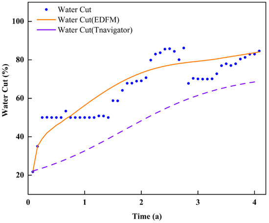
Figure 13.
The water cut curves of well P1 in different reservoir simulators.
4. Conclusions
In this paper, we have achieved the following accomplishments:
- (1)
- We have developed a fracture propagation model that combines the KGD model and the oil–water two-phase flow model to characterize the dynamic fracture finely. The fracture propagation model is verified against the KGD analytical model, and the results show that the fracture propagation length is consistent in different models.
- (2)
- Under constant pressure injection conditions, the fracture length increases quickly at an early time, followed by a slowdown in growth rate later. The injection pressure exhibits small fluctuations, and the time interval of the fluctuations becomes longer.
Under the existing injector–producer conditions, the cumulative oil production rapidly increases within the injection pressure range of 36 MPa to 46 MPa, and slowly increases in other pressure ranges.
- (3)
- The field experiment results show that our fracture propagation model has better fitting results with the on-site water cut curve than a conventional reservoir numerical simulator.
Author Contributions
Conceptualization, D.S.; methodology, D.S.; software, D.S.; validation, D.S., W.B. and X.L.; formal analysis, S.C.; investigation, D.C.; resources, X.L.; data curation, W.B.; writing—original draft preparation, W.B.; writing—review and editing, W.B.; visualization, X.L.; supervision, S.C.; project administration, S.C.; funding acquisition, S.C. All authors have read and agreed to the published version of the manuscript.
Funding
This work is supported by the National Natural Science Foundation of China’s “Mechanism and inversion method of micro fractures induced by water injection in tight oil reservoirs” (11872073).
Data Availability Statement
All data included in this study are available upon request by contact with the corresponding author.
Acknowledgments
Thanks for the support of the MATLAB Reservoir Simulation Toolbox (MRST) in this work.
Conflicts of Interest
The authors declare no conflict of interest.
References
- Li, Q.; Wang, Y.; Wang, F.; Wu, J.; Usman Tahir, M.; Li, Q.; Yuan, L.; Liu, Z. Effect of thickener and reservoir parameters on the filtration property of CO2 fracturing fluid. Energy Sources Part A Recovery Util. Environ. Eff. 2020, 42, 1705–1715. [Google Scholar]
- Yan, B.; Liu, H.; Peng, X. Scenario analysis to evaluate the economic benefits of tight oil resource development in China. Energy Strategy Rev. 2024, 51, 101318. [Google Scholar]
- Lai, F.; Li, Z.; Wei, Q.; Zhang, T.; Zhao, Q. Experimental Investigation of Spontaneous Imbibition in a Tight Reservoir with Nuclear Magnetic Resonance Testing. Energy Fuels 2016, 30, 8932–8940. [Google Scholar] [CrossRef]
- Zhao, J.; Fan, J.; He, Y.; Yang, Z.; Gao, W.; Gao, W. Optimization of Horizontal Well Injection-Production Parameters for Ultra-Low Permeable–Tight Oil Production: A Case from Changqing Oilfield, Ordos Basin, NW China. Pet. Explor. Dev. 2015, 42, 74–82. [Google Scholar]
- Wei, C.; Liu, Y.; Deng, Y.; Cheng, S.; Hassanzadeh, H. Temperature Transient Analysis of Naturally Fractured Geothermal Reservoirs. SPE J. 2022, 27, 2723–2745. [Google Scholar]
- Bai, W.; Cheng, S.; Wang, X.G.Q. A transient production prediction method for tight condensate gas wells with multiphase flow. Pet. Explor. Dev. 2024, 51, 172–179. [Google Scholar]
- Bai, W.; Cheng, S.; Cai, D.; Guo, Q.; Guo, X.; Wang, Y. Integrated Analysis of Two-Phase Production Data in Hydraulic Fractured Deep Shale Reservoirs: Coupling Multiple Fluid Transport Mechanisms. Energy Fuels 2024, 38, 10826–10840. [Google Scholar]
- Wei, C.; Tan, Z.; Huang, G.; Cheng, X.; Zeng, Y.; Luo, H.; Li, Y.; Li, H. Generalized Analytical Well-Test Solutions for Vertically Fractured Wells in Commingled Reservoirs. ASME. J. Energy Resour. Technol. 2023, 146, 053501. [Google Scholar] [CrossRef]
- Adachi, A.; Siebrits, E.; Peirce, A.; Desroches, J. Computer Simulation of Hydraulic Fractures. Int. J. Rock Mech. Min. Sci. 2007, 44, 739–757. [Google Scholar] [CrossRef]
- Secchi, S.; Schrefler, B.A. A Method for 3-D Hydraulic Fracturing Simulation. Int. J. Fract. 2012, 178, 245–258. [Google Scholar] [CrossRef]
- McClure, M.; Babazadeh, M.; Shiozawa, S.; Huang, J. Fully Coupled Hydromechanical Simulation of Hydraulic Fracturing in 3D Discrete-Fracture Networks. SPE J. 2016, 21, 1302–1320. [Google Scholar] [CrossRef]
- Lei, Q.; Gholizadeh Doonechaly, N.; Tsang, C.-F. Modelling Fluid Injection-Induced Fracture Activation, Damage Growth, Seismicity Occurrence and Connectivity Change in Naturally Fractured Rocks. Int. J. Rock Mech. Min. Sci. 2021, 138, 104598. [Google Scholar] [CrossRef]
- Christianovich, S.A.; Zheltov, Y.P. Formation of Vertical Fractures by Means of a Highly Viscous Fluid. In Proceedings of the 4th World Petroleum Congress, Rome, Italy, 6–15 June 1955; Volume 2, pp. 579–586. [Google Scholar]
- Geertsma, J.; De Klerk, F. A Rapid Method of Predicting Width and Extent of Hydraulically Induced Fractures. J. Pet. Technol. 1969, 21, 1571–1581. [Google Scholar] [CrossRef]
- Sharma, S.; Chaudhary, A.; Nair, R. Modeling and Simulation of Reservoir Poroelastic Response during Hydraulic Fracturing. In Proceedings of the International Conference and Exhibition, Barcelona, Spain, 3–6 April 2016; Society of Exploration Geophysicists and American Association of Petroleum Geologists: Barcelona, Spain, 2016; p. 208. [Google Scholar] [CrossRef]
- Wang, Y.; Cheng, S.; Zhang, K.; He, Y.; Yu, H. Pressure-Transient Analysis of Water Injectors Considering the Multiple Closures of Waterflood-Induced Fractures in Tight Reservoirs: Case Studies in Changqing Oilfield, China. J. Pet. Sci. Eng. 2019, 172, 643–653. [Google Scholar] [CrossRef]
- Zhang, F.; Emami-Meybodi, H. A Semianalytical Method for Two-Phase Flowback Rate-Transient Analysis in Shale Gas Reservoirs. SPE J. 2020, 25, 1599–1622. [Google Scholar] [CrossRef]
- Lei, Z.; Tian, C.; Wang, F.; Wang, W.; Peng, H.; Wang, T.; Li, Q.; Yu, Z. A Dynamic Discrete Fracture Model for Simulation of Tight Low-Permeability Reservoirs. In All Days; IPTC: Kuala Lumpur, Malaysia, 2014; p. IPTC-17992-MS. [Google Scholar] [CrossRef]
- Lei, Z.; Xie, Q.; Tao, Z.; He, Y.; Zhu, Z.; Peng, Y.; Liu, C. Waterflooding Management and Optimization for Reservoir Simulation with Coupled Geomechanics and Dynamic Fractures Using Streamline-Based Information. In Proceedings of the SPE Europec Featured at 81st EAGE Conference and Exhibition, London, UK, 3–6 June 2019; SPE: London, UK, 2019; p. D021S001R010. [Google Scholar] [CrossRef]
- Yang, C.; Cheng, L.; Cao, R.; Shi, J.; Du, X. An Improved Embedded Discrete Fracture Model with Fracture Growth for Water-Induced Fracture Simulation in Low Permeability Reservoirs. Lithosphere 2022, 2021, 2882368. [Google Scholar] [CrossRef]
- Rao, X.; Cheng, L.; Cao, R.; Jia, P.; Du, X. A Fast Embedded Discrete Fracture Model Based on Proper Orthogonal Decomposition POD Method. In Proceedings of the SPE Kuwait Oil & Gas Show and Conference, Mishref, Kuwait, 13–16 October 2019; SPE: Mishref, Kuwait, 2019; p. D023S004R006. [Google Scholar] [CrossRef]
- Samy, A. Wellbore Strengthening Uncertainties and Workflow Optimizations. In Proceedings of the International Petroleum Technology Conference, Dhahran, Saudi Arabia, 12 February 2024; IPTC: Dhahran, Saudi Arabia, 2024; p. D011S017R007. [Google Scholar] [CrossRef]
- Li, Z.; Luo, H.; Bhardwaj, P.; Wang, B.; Delshad, M. Modeling Dynamic Fracture Growth Induced by Non-Newtonian Polymer Injection. J. Pet. Sci. Eng. 2016, 147, 395–407. [Google Scholar] [CrossRef]
- Lujun, J.; Settari, A.T.; Sullivan, R.B.; Orr, D. Methods for modeling dynamic fractures in coupled reservoir and geomechanics simulation. In Proceedings of the SPE Annual Technical Conference and Exhibition, Houston, TX, USA, 26–29 September 2004. Society of Petroleum Engineers. [Google Scholar]
- Gadde, P.B.; Sharma, M.M. Growing injection well fractures and their impact on waterflood performance. In Proceedings of the SPE Annual Technical Conference and Exhibition, New Orleans, LA, USA, 30 September–3 October 2001. Society of Petroleum Engineers. [Google Scholar]
- Lie, K.-A. An Introduction to Reservoir Simulation Using MATLAB/GNU Octave: User Guide for the MATLAB Reservoir Simulation Toolbox (MRST); Cambridge University Press: Cambridge, UK, 2019; Available online: https://www.cambridge.org/9781108492430 (accessed on 8 August 2019).
- Bao, K.; Lie, K.A.; Møyner, O.; Liu, M. Fully implicit simulation of polymer flooding with MRST. Comput. Geosci. 2017, 21, 1219–1244. [Google Scholar]
- Zhang, F.; Wu, S.; Liu, H. A Waterflood Induced Fracture Simulation Model for Naturally Fractured Low-Permeability Reservoirs. In Proceedings of the SPE Asia Pacific Oil & Gas Conference and Exhibition, Perth, Australia, 25–27 October 2016. [Google Scholar] [CrossRef]
- Du, K.; Rui, Z.; Dindoruk, B.; Yang, T.; Patil, S. A Mathematical Model and Numerical Simulation of Waterflood Induced Dynamic Fractures of Low Permeability Reservoirs. In Proceedings of the SPE Asia Pacific Oil and Gas Conference and Exhibition, Jakarta, Indonesia, 10–12 October 2023; p. D011S002R003. [Google Scholar]
- Tianyi, F.; Shuhong, W.; Hua, L.; Baohua, W.; Xiaobo, L. A Dynamic Hybrid Dual Porosity Model to Simulate the Waterflood-Induced Fractures in Low-Permeability Reservoir. In Proceedings of the SPE Asia Pacific Oil & Gas Conference & Exhibition, Jakarta, Indonesia, 17–19 October 2017. [Google Scholar] [CrossRef]


Disclaimer/Publisher’s Note: The statements, opinions and data contained in all publications are solely those of the individual author(s) and contributor(s) and not of MDPI and/or the editor(s). MDPI and/or the editor(s) disclaim responsibility for any injury to people or property resulting from any ideas, methods, instructions or products referred to in the content. |
© 2024 by the authors. Licensee MDPI, Basel, Switzerland. This article is an open access article distributed under the terms and conditions of the Creative Commons Attribution (CC BY) license (https://creativecommons.org/licenses/by/4.0/).