Research on Energy Dissipation of Hydrofoil Cavitation Flow Field with FBDCM Model

Abstract

In order to obtain a more detailed and comprehensive relationship between the cavitation phenomenon and energy loss, this paper takes an NACA66 hydrofoil as an example to analyze the specific relationship between the cavitation flow field and energy dissipation by using entropy production theory, a ZGB cavitation model, and k-ε turbulence model which were modified by a Filter-Based Density Correction model (FBDCM). The results show that the modified k-ε model can effectively capture the morphology of cavity evolution in the cavitation flow field. The vortex dilatation term contributes the most to the vorticity transport in cavitation flow. The energy loss of the cavitation flow field is primarily composed of turbulent dissipation, which is primarily distributed in the area below the lifted attached cavity and inside the vortex induced by the cloud cavity. The direct dissipation entropy production is predominantly distributed in the area near the stagnation point of the hydrofoil’s leading edge and inside the cavity. The wall entropy production is chiefly distributed in the area where the cavity is not covered. The cavitation entropy production mainly occurs on the vapor–liquid interface, and the value is negative, indicating that the vapor–liquid conversion in the cavitation process needs to absorb energy from the flow field.

1. Introduction

Cavitation occurs primarily in regions where the local pressure drops below the corresponding saturation vapor pressure at a specific temperature. It is a kind of multi-scale vapor–liquid flow that involves unsteady characteristics such as vapor–liquid mass transfer, compressibility, vortex evolution, turbulent viscosity effects, etc. The unsteady phenomenon of cavitation flow includes the dynamic cyclic process of inception, development, fracture, discharge, collapse, and regeneration of the cavity. Cavitation flow has beneficial effects in certain situations. The accompanying high-frequency noise can be used for the early diagnosis of cavitation problems and early warning of potential mechanical damages [1]. However, cavitation flow is always accompanied by abrupt load changes, resulting in pressure ripples, cavitation erosion, efficiency reduction, noise, vibration, and other hazards, thus affecting the safe and stable operation of fluid machinery.

The cavitation phenomenon in fluid machinery inevitably leads to energy loss [2]. With the aim of evaluating the energy loss of the flow field, the pressure drop method, Darcy’s formula, and the exergy equilibrium method are usually used. For these three types of methods, local energy losses such as viscous dissipation and turbulent dissipation cannot be quantitatively obtained. However, the combination of a CFD numerical simulation [3] and an entropy production analysis is a new method for quantifying local and overall hydraulic losses. CFD simulation can save a lot of experimental time and cost and can obtain information that cannot be obtained from experiments. The combined method can reveal the irreversible extent of the evolution of the flow field, visually display the area of flow deterioration, and identify specific locations where energy loss occurs. To quantitatively evaluate the energy loss in the flow field, many researchers have established an inherent connection between the local entropy production rate and hydraulic loss in fluid mechanical systems. Bejan et al. [4] initially proposed the idea of minimizing entropy production and analyzed the reasons for entropy production during heat transfer in single-phase flow fields. Kock et al. [5] time-averaged the transport equation for entropy production and classified its occurrences in single-phase flow fields. Wang Wei et al. [6] used different turbulence models to simulate the entropy generation rate of a single-phase flow field around a two-dimensional hydrofoil and pointed out that the energy loss of the flow field primarily occurs at the hydrofoil’s leading edge, the boundary layer of the upper wall surface, and the wake region. They also declared that the turbulent dissipation dominates the production of entropy. In the cavitation flow field, Zhang Yatai et al. [7] analyzed the correlation between the entropy production and the external characteristics of the hydrofoil and observed that the energy loss in the cavitation flow field is generally concentrated at the rear of the cavity and the trailing of the hydrofoil. Yu An et al. [8] analyzed the entropy production caused by direct dissipation, turbulent dissipation, wall shear stress, the average temperature gradient, and fluctuating temperature gradient in an unsteady cavitation flow at 70 °C and studied the interaction between entropy production and cavitation. The results indicate that the direct dissipation of entropy production better reflects the overall pattern of the total entropy production, and that the velocity gradient, as well as phase transition, are important factors to control the entropy changes.

A suitable turbulence model plays a crucial role in feature capture for cavitation flows [9,10]. The LES model is very accurate in simulating cavitation structures and turbulent flow states, but it requires many grids and a very small time step, which is not convenient for engineering calculations. The RANS model has a small computational load; however, it can over predict the turbulent viscosity of the cavity tail, resulting in a much larger viscous force at the tailing of the cavity, which hinders the upstream development of the re-entrant jet. Therefore, the turbulent viscosity of the RANS model needs to be adjusted to enhance the reliability of simulating cavitation flow.

There are two main viscosity correction methods for the RANS model: one is the filter model (FBM), which corrects turbulent viscosity through filter scale [11], and the other is the density correction model (DCM), which considers the compressibility characteristics of vapor–liquid mixtures [12]. Based on the FBM, Liu Lu et al. [13] studied the cloud cavity evolution process, shedding frequency, lift coefficient, and hydrofoil surface velocity gradient distribution around the Clark-Y hydrofoil. The results show that the FBM effectively weakens the turbulent viscosity far away from the wall, but the simulation of the cavity evolution process in the near-wall region is poor. Yin Tingyun et al. [14] studied the cavitation flow around a three-dimensional Clark-Y hydrofoil with the DCM. Their research findings indicate that the periodic initiation, shedding, and collapse of the hydrofoil are in good agreement with the experiment. For the purpose of obtaining a more accurate reflection of the flow state across the entire flow field, Huang Biao et al. [15] developed the Filter-Based Density Correction model (FBDCM), based on the combination of the FBM and the DCM. This model can simultaneously account for the effects of turbulent viscosity and density fluctuations in numerical simulations of cavitation flow, ultimately capturing the interactions and dynamic behaviors between turbulence and cavitation. Huang Biao et al. [16] used the FBDCM to predict the cavity morphology of Clark-Y hydrofoils under a certain operating condition. The results indicate that the FBDCM reduces the impact of turbulent viscosity within the cavity, more accurately obtains the characteristics of the unsteady evolution of the cavity, and captures the interaction, as well as the dynamic behavior, between turbulence and cavitation. Chen Guanghao [17] adopted the FBDCM and ZGB cavitation model [18] for simulating the two-phase turbulence around the Clark-Y hydrofoil. The model is in good agreement with experiments in predicting the time-averaged lift, drag coefficient, and shedding frequency. The accuracy of the FBDCM in the numerical simulation of cavitation flow has also been confirmed by other scholars [19,20].

Although previous scholars have studied the cavitation flow field and energy dissipation law, the dynamic characteristics of the entropy production rate in a cavitation flow field and its relationship with transient flow structure are still unclear. This paper uses numerical methods to study the relationship between vortex evolution, cavity morphology, the vapor–liquid phase transition process, and energy loss in the flow field. The organizational structure of this article is as follows: Section 2 introduces the numerical model and software settings for hydrodynamic simulations. In Section 3, the interaction between cavitation and vortexes during the evolution process was analyzed and discussed, and the relationship between the entropy generation rate distribution and flow structure was obtained. Section 4 summarizes the main conclusions.

2. Numerical Model

2.1. Governing Equations

This paper assumes that the two-phase flow involved is homogeneous flow. The governing equations, namely, Favre-averaged continuity and momentum equations, are represented as follows [16]:

$${\displaystyle \frac{\partial {\rho }_{\mathrm{m}}}{\partial t}}+{\displaystyle \frac{\partial \left({\rho }_{\mathrm{m}}{u}_{\mathrm{j}}\right)}{\partial x_{\mathrm{j}}}}=0$$

(1)

$${\displaystyle \frac{\partial \left({\rho }_{\mathrm{m}}{u}_{\mathrm{i}}\right)}{\partial t}}+{\displaystyle \frac{\partial \left({\rho }_{\mathrm{m}}{u}_{\mathrm{i}}{u}_{\mathrm{j}}\right)}{\partial x_{\mathrm{j}}}}=-{\displaystyle \frac{\partial p}{\partial x_{\mathrm{i}}}}+{\displaystyle \frac{\partial }{\partial x_{\mathrm{j}}}}\left[\left(\mu +{\mu }_{\mathrm{t}}\right)\left({\displaystyle \frac{\partial u_{\mathrm{i}}}{\partial x_{\mathrm{j}}}}+{\displaystyle \frac{\partial u_{\mathrm{j}}}{\partial x_{\mathrm{i}}}}-{\displaystyle \frac{2}{3}}{\displaystyle \frac{\partial u_{\mathrm{i}}}{\partial x_{\mathrm{j}}}}{\delta }_{\mathrm{ij}}\right)\right]$$

(2)

$${\rho }_{\mathrm{m}}={\rho }_{\mathrm{l}}{\alpha }_{\mathrm{l}}+{\rho }_{\mathrm{v}}{\alpha }_{\mathrm{v}}$$

(3)

where subscripts i and j indicate the coordinate directions; ρ_m, u, and p represent the density, velocity, and pressure of the mixed phase, respectively; μ and μ_t are the laminar and turbulent viscosities of the vapor–liquid mixture, respectively; ρ_l means the density of water; and ρ_v is the density of vapor.

2.2. Filter-Based Density Modified Model

In this research, the standard k-ε model was employed as the turbulence model. The specific expression is as follows [16]:

$${\displaystyle \frac{\partial \left({\rho }_{\mathrm{m}}k\right)}{\partial t}}+{\displaystyle \frac{\partial \left({\rho }_{\mathrm{m}}{u}_{\mathrm{j}}k\right)}{\partial x_{\mathrm{j}}}}=P_{\mathrm{t}}-{\rho }_{\mathrm{m}}\epsilon +{\displaystyle \frac{\partial }{\partial x_{\mathrm{j}}}}\left[\left(\mu +{\displaystyle \frac{{\mu }_{\mathrm{t}}}{{\sigma }_{\mathrm{k}}}}\right){\displaystyle \frac{\partial k}{\partial x_{\mathrm{j}}}}\right]$$

(4)

$${\displaystyle \frac{\partial \left({\rho }_{\mathrm{m}}\epsilon \right)}{\partial t}}+{\displaystyle \frac{\partial \left({\rho }_{\mathrm{m}}{u}_{\mathrm{j}}\epsilon \right)}{\partial x_{\mathrm{j}}}}=C_{\epsilon 1}{\displaystyle \frac{\epsilon }{k}}{P}_{\mathrm{t}}-C_{\epsilon 2}{\rho }_{\mathrm{m}}{\displaystyle \frac{{\epsilon }^2}{k}}+{\displaystyle \frac{\partial }{\partial x_{\mathrm{j}}}}\left[\left(\mu +{\displaystyle \frac{{\mu }_{\mathrm{t}}}{{\sigma }_{\epsilon }}}\right){\displaystyle \frac{\partial \epsilon }{\partial x_{\mathrm{j}}}}\right]$$

(5)

where C_μ is 0.09, k represents turbulent kinetic energy; ε denotes the turbulent dissipation rate; and P_t is the turbulent kinetic energy generation term. The values of the model parameters, C_ε1, C_ε2, σ_ε, and σ_k are 1.44, 1.92, 1.3, and 1.0, respectively.

The vortex viscosity coefficient μ_t in Equations (4) and (5) can be obtained by the Equation (6) [16]:

$${\mu }_{\mathrm{t}}=C_{\mathsf{\mu }}{\rho }_{\mathrm{m}}{\displaystyle \frac{k^2}{\epsilon }}$$

(6)

The FBDCM is utilized to correct the μ_t:

$${\mu }_{\mathrm{T}\text{\_}\mathrm{hybrid}}={\displaystyle \frac{C_{\mathsf{\mu }}{\rho }_{\mathrm{m}}{k}^2}{\epsilon }}{f}_{\mathrm{hybrid}}$$

(7)

$$f_{\mathrm{hybrid}}=\chi \left({\rho }_{\mathrm{m}}/{\rho }_{\mathrm{l}}\right)f_{\mathrm{FBM}}+\left[1-\chi \left({\rho }_{\mathrm{m}}/{\rho }_{\mathrm{l}}\right)\right]f_{\mathrm{DCM}}$$

(8)

$$\chi \left({\rho }_{\mathrm{m}}/{\rho }_{\mathrm{l}}\right)=0.5+\tan \mathrm{h}\left[{\displaystyle \frac{C_1\left(0.6{\rho }_{\mathrm{m}}/{\rho }_{\mathrm{l}}-C_2\right)}{0.2\left(1-2C_2\right)+C_2}}\right]/\left[2\tan \mathrm{h}\left(C_1\right)\right]$$

(9)

where μ_{T_hybrid} is the corrected turbulent viscosity, and f_hybrid is the transition function; the values of C₁ and C₂ are 4 and 0.2, respectively.

The coefficient f_FBM in Equation (8) is derived from the FBM, and can be obtained by equations as follows:

$$f_{\mathrm{FBM}}=\min \left(1,{\displaystyle \frac{\Delta \epsilon }{k^{3/2}}}\right)$$

(10)

$$\Delta ={\left({\Delta }_{\mathrm{x}}{\Delta }_{\mathrm{y}}{\Delta }_{\mathrm{z}}\right)}^{1/3}$$

(11)

where Δ_x, Δ_y, and Δ_z represent the lengths of the grids along the three coordinate directions.

The coefficient f_DCM in Equation (8) originates from the DCM and can be determined by equations as follows:

$$f_{\mathrm{DCM}}={\displaystyle \frac{{\rho }_{\mathrm{v}}+{\left(1-{\alpha }_{\mathrm{v}}\right)}^{\mathrm{n}}\left({\rho }_{\mathrm{l}}-{\rho }_{\mathrm{v}}\right)}{{\rho }_{\mathrm{v}}+\left(1-{\alpha }_{\mathrm{v}}\right)\left({\rho }_{\mathrm{l}}-{\rho }_{\mathrm{v}}\right)}}$$

(12)

where n takes a value of 10 [21].

2.3. Cavitation Model

The Singhal (FCM) model, Zwart–Gerber–Belamri (ZGB) model, and Schnerr–Sauer model have been proposed based on the Rayleigh–Plesset cavity dynamics two-phase flow equation. Among them, the ZGB model focuses on the influence of the cavitation volume change during cavity inception and development, and has been widely used. The ZGB cavitation model is formulated as follows:

$${\displaystyle \frac{\partial \left({\rho }_{\mathrm{v}}{\alpha }_{\mathrm{v}}\right)}{\partial t}}+{\displaystyle \frac{\partial \left({\rho }_{\mathrm{v}}{\alpha }_{\mathrm{v}}{u}_{\mathrm{j}}\right)}{\partial x_{\mathrm{j}}}}=m^{+}-m^{-}$$

(13)

where m⁺ and m⁻ denote the evaporation and condensation source terms, respectively.

When $p\le P_{\mathrm{v}}$, the expression for the evaporation process is as follows:

$$m^{+}=F_{\mathrm{vap}}{\displaystyle \frac{3{\rho }_{\mathrm{v}}{\alpha }_{\mathrm{nuc}}\left(1-{\alpha }_{\mathrm{v}}\right)}{R_{\mathrm{b}}}}\sqrt{{\displaystyle \frac{2}{3}}{\displaystyle \frac{\left(p_{\mathrm{v}}-p\right)}{{\rho }_{\mathrm{l}}}}}$$

(14)

When $p\ge P_{\mathrm{v}}$, the expression for the condensation process is as follows:

$$m^{-}=F_{\mathrm{cond}}{\displaystyle \frac{3{\rho }_{\mathrm{v}}{\alpha }_{\mathrm{v}}}{R_{\mathrm{b}}}}\sqrt{{\displaystyle \frac{2}{3}}{\displaystyle \frac{\left(p_{\mathrm{v}}-p\right)}{{\rho }_{\mathrm{l}}}}}$$

(15)

where α_nuc is the volume fraction of nucleation site, with a value of 5 × 10⁻⁴; R_b is the initial cavity radius at the nucleation site, with a value of 10⁻⁶ m; and F_vap and F_cond are evaporation and condensation coefficients determined based on experience, with values of 50 and 0.01, respectively.

2.4. Entropy Production Equation

According to Bejan et al.’s research [4], entropy production is associated with both turbulence dissipation and heat transfer dissipation. In the process of fluid flow, the turbulence dissipation term arises from the velocity gradients, while the heat transfer dissipation term results from the temperature differences.

In this paper, it is assumed that the temperature of the flow field remains constant. Therefore, the heat dissipation term can be ignored. The expression for the entropy production rate $S_{\mathrm{total}}^{‴}$ per unit volume within a differential element is as follows:

$$S_{\mathrm{total}}^{‴}={\displaystyle \frac{\Phi }{T}}$$

(16)

where T denotes temperature, K; Φ denotes turbulence dissipation term.

Since the turbulence model chosen for this paper is the RANS model, the instantaneous motion is decomposed into mean motion and fluctuating motion. Consequently, the entropy production is primarily composed of the direct dissipation entropy production due to the average velocity and the turbulent dissipation entropy production due to the fluctuating velocity [5]. Moreover, in cavitation flow, there exists a vapor–liquid two-phase transition, necessitating the consideration of entropy production during the phase transition process [22]. The total entropy production rate $S_{\mathrm{total}}^{‴}$ per unit volume can be expressed as follows [5]:

$$S_{\mathrm{total}}^{‴}=S_{\overline{\mathrm{D}}}^{‴}+S_{{\mathrm{D}}^{\prime }}^{‴}+S_{\mathrm{C}}^{‴}$$

(17)

where $S_{\overline{\mathrm{D}}}^{‴}$ is the direct dissipation entropy production rate, W/(m³·K); $S_{{\mathrm{D}}^{\prime }}^{‴}$ is the turbulent dissipation entropy production rate, W/(m³·K); and $S_{\mathrm{C}}^{‴}$ is the cavitation entropy production rate, W/(m³·K).

$S_{\overline{\mathrm{D}}}^{‴}$ can be obtained by equations as follows:

$$S_{\overline{\mathrm{D}}}^{‴}={\displaystyle \frac{{\mu }_{\mathrm{eff}}}{T}}\left[{\left({\displaystyle \frac{\partial \overline{u}}{\partial y}}+{\displaystyle \frac{\partial \overline{v}}{\partial x}}\right)}^2+{\left({\displaystyle \frac{\partial \overline{u}}{\partial z}}+{\displaystyle \frac{\partial \overline{w}}{\partial x}}\right)}^2+{\left({\displaystyle \frac{\partial \overline{w}}{\partial y}}+{\displaystyle \frac{\partial \overline{v}}{\partial z}}\right)}^2\right]+{\displaystyle \frac{2{\mu }_{\mathrm{eff}}}{T}}\left[{\left({\displaystyle \frac{\partial \overline{u}}{\partial x}}\right)}^2+{\left({\displaystyle \frac{\partial \overline{v}}{\partial y}}\right)}^2+{\left({\displaystyle \frac{\partial \overline{w}}{\partial z}}\right)}^2\right]$$

(18)

$S_{\mathrm{C}}^{‴}$ can be obtained by equations as follows:

$$S_{{\mathrm{D}}^{\prime }}^{‴}={\displaystyle \frac{{\mu }_{\mathrm{eff}}}{T}}\left[{\left({\displaystyle \frac{\partial u^{\prime }}{\partial y}}+{\displaystyle \frac{\partial v^{\prime }}{\partial x}}\right)}^2+{\left({\displaystyle \frac{\partial u^{\prime }}{\partial z}}+{\displaystyle \frac{\partial w^{\prime }}{\partial x}}\right)}^2+{\left({\displaystyle \frac{\partial w^{\prime }}{\partial y}}+{\displaystyle \frac{\partial v^{\prime }}{\partial z}}\right)}^2\right]+{\displaystyle \frac{2{\mu }_{\mathrm{eff}}}{T}}\left[{\left({\displaystyle \frac{\partial u^{\prime }}{\partial x}}\right)}^2+{\left({\displaystyle \frac{\partial v^{\prime }}{\partial y}}\right)}^2+{\left({\displaystyle \frac{\partial w^{\prime }}{\partial z}}\right)}^2\right]$$

(19)

$S_{\mathrm{C}}^{‴}$ can be obtained by equations as follows:

$$S_{\mathrm{C}}^{‴}=-{\displaystyle \frac{2}{3}}{\displaystyle \frac{{\mu }_{\mathrm{eff}}}{T}}\left(\nabla \cdot \mathrm{v}\right)=-{\displaystyle \frac{2}{3}}{\displaystyle \frac{{\mu }_{\mathrm{eff}}}{T}}{\left[\dot{m}\left({\displaystyle \frac{1}{{\rho }_{\mathrm{l}}}}-{\displaystyle \frac{1}{{\rho }_{\mathrm{v}}}}\right)\right]}^2$$

(20)

where $\overline{u}$, $\overline{v}$, and $\overline{w}$ are the components of average velocity in the x, y, and z directions, m/s; u′, v′, and w′ are the components of fluctuating velocity in the x, y and z directions, m/s; μ_eff is the effective dynamic viscosity of the fluid, and Pa·s; $\dot{m}$ represents the mass transfer rate between water and vapor, kg/(m³·s).

Since the Reynolds average method is used in this paper, extracting the fluctuating velocity component from the Equation (19) is challenging. The turbulent dissipation entropy production rate $S_{{\mathrm{D}}^{\prime }}^{‴}$ can be calculated by the following equation [23]:

$$S_{{\mathrm{D}}^{\prime }}^{‴}={\displaystyle \frac{{\rho }_{\mathrm{m}}\epsilon }{T}}$$

(21)

Furthermore, Kock et al. [24] demonstrated that applying the entropy production formula directly at the wall would result in significant errors due to the existence of wall friction. Therefore, Zhang Xiang et al. [25] proposed a method to calculate the wall entropy production rate $S_{\mathrm{W}}^{″}$ using wall shear stress, as shown in the following equation:

$$S_{\mathrm{W}}^{″}={\displaystyle \frac{\tau \cdot v}{T}}$$

(22)

where τ is the wall shear stress, Pa; ν is the average velocity of the fluid at the center of the first grid layer along the hydrofoil surface, m/s.

The direct dissipation entropy production value $S_{\overline{\mathrm{D}}}$ (W/K), turbulent dissipation entropy production value $S_{{\mathrm{D}}^{\prime }}$ (W/K), cavitation entropy production value $S_{\mathrm{C}}$ (W/K), and wall entropy production value $S_{\mathrm{w}}$ (W/K) can be expressed by integrating the above entropy production rate per unit volume:

$$S_{\overline{\mathrm{D}}}={\displaystyle {\int }_V{S}_{\overline{\mathrm{D}}}^{‴}}\mathrm{d}V$$

(23)

$$S_{{\mathrm{D}}^{\prime }}={\displaystyle {\int }_V{S}_{{\mathrm{D}}^{\prime }}^{‴}}\mathrm{d}V$$

(24)

$$S_{\mathrm{C}}={\displaystyle {\int }_V{S}_{\mathrm{C}}^{‴}}\mathrm{d}V$$

(25)

$$S_{\mathrm{w}}={\displaystyle {\int }_S{S}_{\mathrm{W}}^{″}}\mathrm{d}S$$

(26)

where V and S, respectively, denote the volume and the area of the over-current.

After considering the cavitation entropy, the total entropy production value calculation equation is as follows:

$$S_{\mathrm{total}}=S_{\overline{\mathrm{D}}}+S_{{\mathrm{D}}^{\prime }}+S_{\mathrm{C}}+S_{\mathrm{w}}$$

(27)

2.5. Geometric Dimensions Fluid Domain and Software Settings

The hydrofoil studied in this paper was an NACA66, which is the same as the experimental size of the reference [26]. The thickest part of the hydrofoil was positioned 45% along its chord length, with a thickness-to-chord ratio of 12%. The maximum camber ratio was situated 50% along the chord length, with a camber-to-chord ratio of 2%. The chord length of the hydrofoil c was 0.075 m, the span length b was 0.069 m, and the angle of attack α was 8°. The length and height of the computational domain ware set to 10 times chord length and 2.5 chord length, respectively. The distance between the trailing edge of the hydrofoil and the outlet was 5 times chord length. The cavitation number $\sigma =\left(p_{\infty }-p_{\mathrm{v}}\right)/\left(0.5{\rho }_{\mathrm{l}}{u}_{\infty }^2\right)$, and the static pressure outlet p_∞ were calculated by the cavitation number. The velocity inlet was a uniform flow, with turbulence intensity I = 1%. The physical properties of liquid water and water vapor in the simulation were based on their physical properties at 25 °C. The saturated vapor pressure p_v was 3169 Pa. All the walls, including hydrofoils, were adiabatic and slip free. There was a 1 mm gap between the left wall of the fluid domain and the left side of the hydrofoil. The Reynolds number (Re) of incoming flow was 6 × 10⁵ and the cavitation number σ was 0.8. The three-dimensional hydrofoil computational domain is displayed in Figure 1.

Currently, Ansys Fluent offers numerous physical models and accurate numerical solution methods. Therefore, this research employed the commercial software Ansys Fluent (2020 R2) software (Canonsburg, PA, USA). The convergence residual was set to 10⁻⁶. The first-order implicit scheme was used to discretize the transient term. The velocity pressure coupling relationship was solved using the SIMPLE algorithm to obtain more accurate results. The PRESTO scheme was used to solve the pressure equation. In order to ensure the accuracy of the simulation, the second-order scheme was used for solving the volume fraction of the cavitation model. To guarantee the calculation stability during the simulation, the Courant number (Co) was set to be less than 1. Therefore, the time step could be obtained by equation Δt = T_ref/200 = 4.7 × 10⁻⁵ s, where T_ref = c/u_∞.

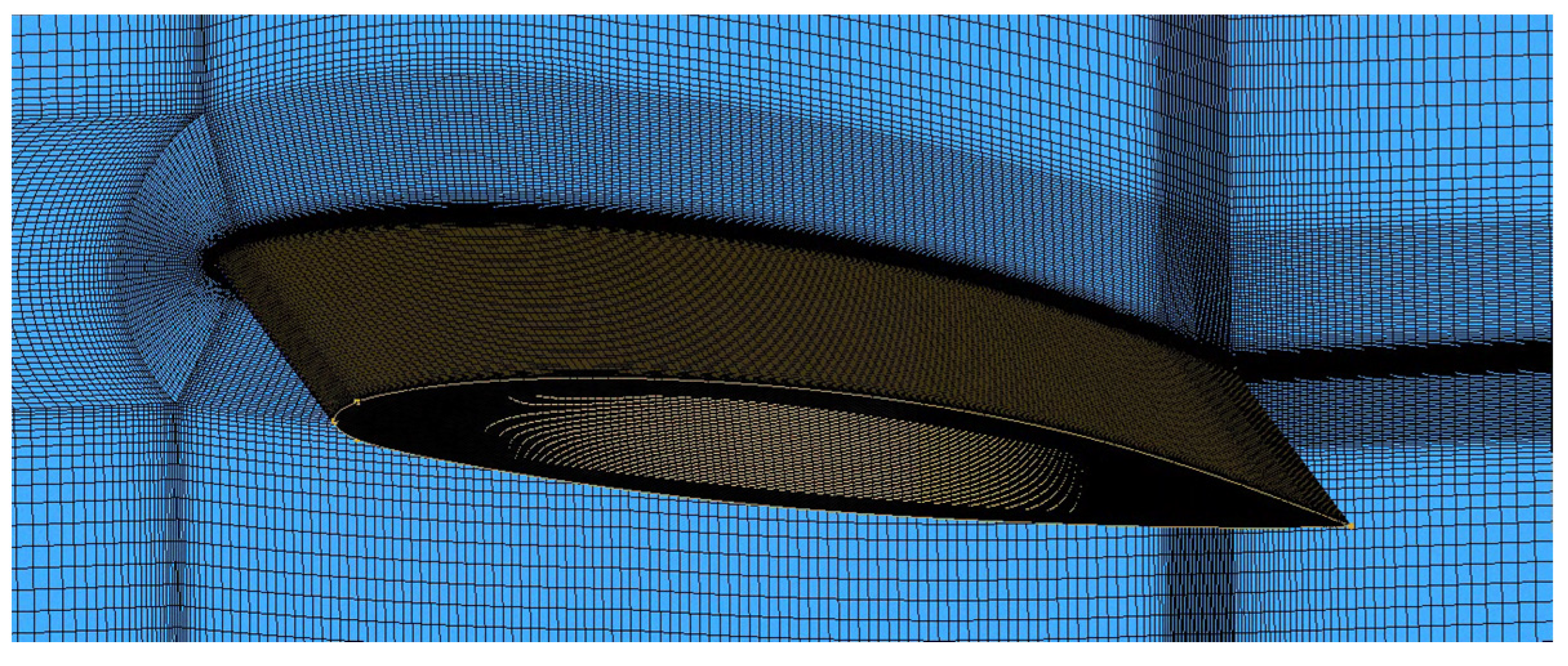
2.6. Grid Generation and Independence Verification

This article used ANSYS ICEM CFD (2020 R2) software (Canonsburg, PA, USA) to discretize the structured mesh of a computational domain with a 1 mm gap. In order to better match the shape of the hydro-foil and the flow domain, the grid adopted an O-H topology structure. For accurately obtaining the cavitation characteristics, an enhanced wall function was applied to solve the viscous bottom layer. The vicinity of the hydrofoil was a prism layer grid, which was divided into 80 layers. The first layer grid height was 2.8 × 10⁻⁶ mm, and the growth rate of the prism layer grid was 1.1. The dimensionless distance of y⁺ of the hydrofoil surface was about 1, which is suitable for simulating the inception and detachment of a cavity near the wall. Figure 2 shows the mesh details of the hydrofoil surface.

In the verification of grid independence, this study set 20, 55, 90, or 125 nodes along the hydrofoil span direction, and generated 4 sets of grids with different numbers. In this case, the hydrofoil attack angle was 8°, the cavitation number σ was 0.8, and the Reynolds number was 6 × 10⁵. The time-averaged lift and drag coefficients, as well as the cavitation shedding frequency, were adopted as the verification indexes. The expressions of time-averaged lift and drag coefficients were as follows:

$$C_{\mathrm{L}}={\displaystyle \frac{F_{\mathrm{L}}}{0.5{\rho }_{\mathrm{l}}{u}_{\infty }^{2}cb}}$$

(28)

$$C_{\mathrm{D}}={\displaystyle \frac{F_{\mathrm{D}}}{0.5{\rho }_{\mathrm{l}}{u}_{\infty }^{2}cb}}$$

(29)

where F_L is the lift force, F_D is the drag force, c is the chord length, and b is the span length.

The number of grids and the simulation results of the four sets of grids are shown in

Table 1. Mesh independence verification results.

	Number of Cells	CL	CD	f
M1	3,036,694	0.602	0.085	18.25
M2	5,618,224	0.608	0.087	18.11
M3	8,199,754	0.614	0.088	18.09
M4	10,781,284	0.616	0.088	18.08
Exp. [26]	-	0.620	0.090	18.05

. After simulation, the time-averaged lift coefficient, drag coefficient, and cavity shedding frequency of the M3 and M4 grids were very close to the experimental results [26]. Considering both the computational time and numerical accuracy, this paper used an M3 grid for the subsequent numerical simulation.

Figure 3 compares the experimental results of reference [26] with the simulation results of the M3 grid in this paper. The lift coefficient normalized power spectral density simulated in this article clearly shows a dominant frequency, which is consistent with the experimental results [26].

According to Table 1 and Figure 3, the simulation model in this paper is accurate and suitable for analyzing the dynamic behavior of the cavitation flow field and energy loss.

3. Results and Discussion

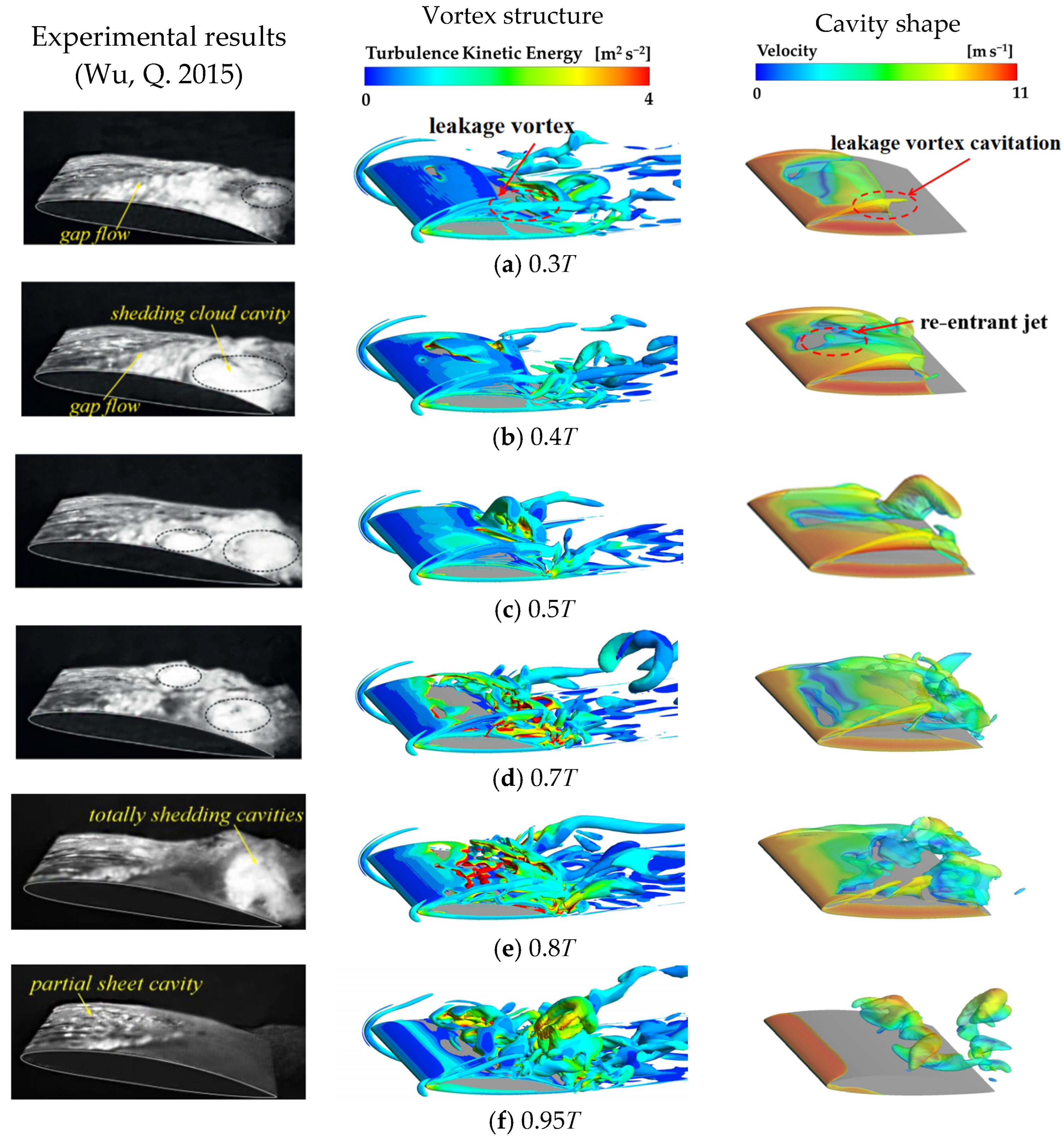
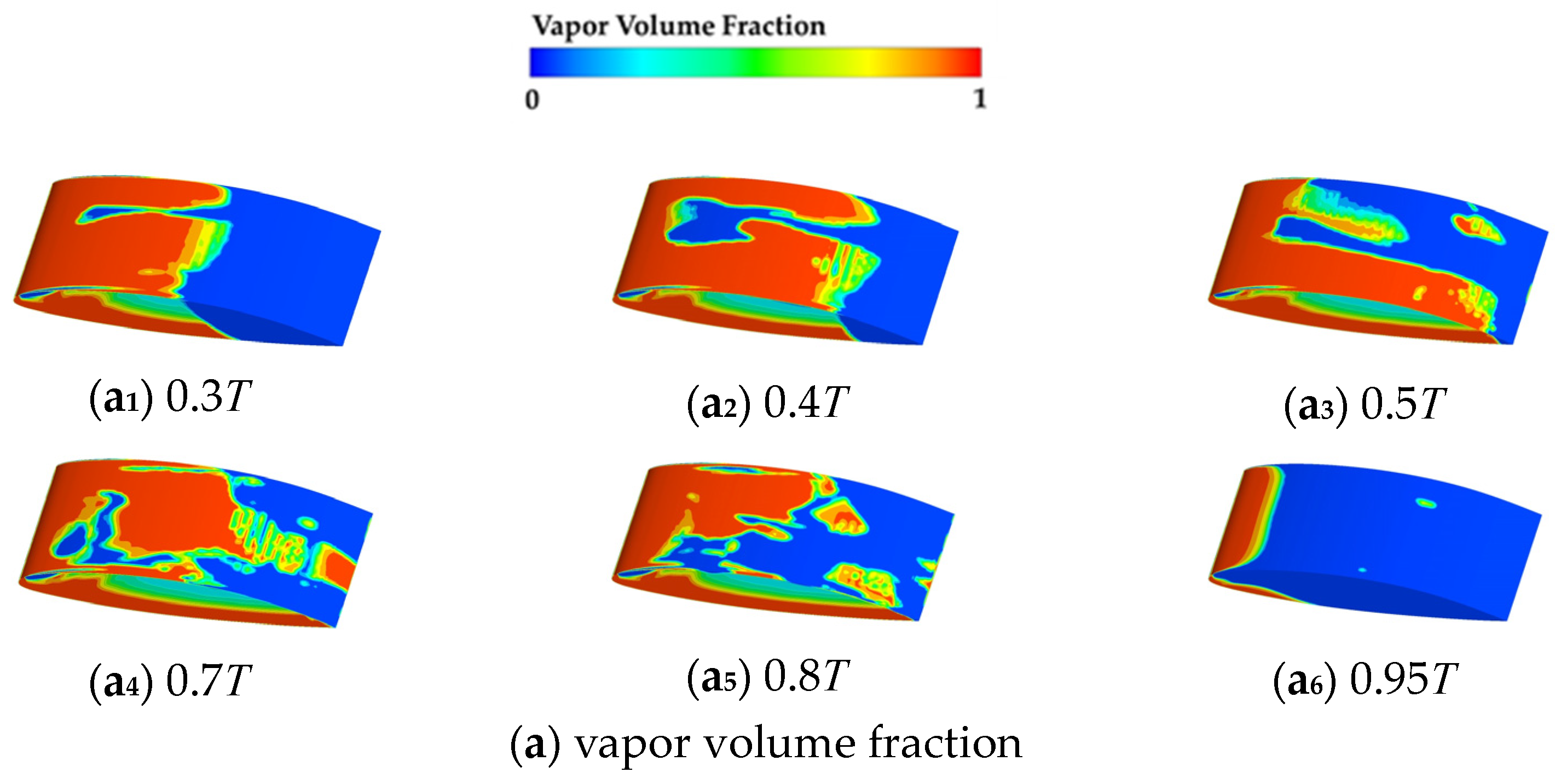
3.1. Vortex and Cavity

To accurately identify the vortex structure in the three-dimensional cavitation flow field, the Q-criterion was applied in this paper. The Q-criterion decomposes the local velocity gradient, tensor D_ij, into a symmetric tensor S_ij (S_ij represents the fluid deformation effect) and an antisymmetric tensor ꞷ_ij (ꞷ_ij represents the fluid rotation effect). When the antisymmetric tensor exceeds the symmetric tensor, a vortex structure is formed. The relevant formula is as follows:

$$Q={\displaystyle \frac{1}{2}}\left(\left|\right|{\omega }_{\mathrm{ij}}|{|}^2-|\left|S_{\mathrm{ij}}\right|{|}^2\right)$$

(30)

$$S_{\mathrm{ij}}={\displaystyle \frac{1}{2}}\left({\displaystyle \frac{\partial u_{\mathrm{i}}}{\partial x_{\mathrm{j}}}}+{\displaystyle \frac{\partial u_{\mathrm{j}}}{\partial x_{\mathrm{i}}}}\right)$$

(31)

$${\omega }_{\mathrm{ij}}={\displaystyle \frac{1}{2}}\left({\displaystyle \frac{\partial u_{\mathrm{i}}}{\partial x_{\mathrm{j}}}}-{\displaystyle \frac{\partial u_{\mathrm{j}}}{\partial x_{\mathrm{i}}}}\right)$$

(32)

The vortex evolution and the cavity morphology of the cloud cavitation flow field during one period are shown in Figure 4. The threshold of Q was selected as 2 × 10⁵ s⁻², the surface of the vortex structure was colored by turbulent kinetic energy, while the surface of the cavity morphology was colored by velocity.

As shown in the vortex structure in Figure 4, from 0.3T to 0.4T, the attached cavity near the leading edge of the hydrofoil continuously grew downstream. At this time, the main body of the vortex existed near the rear and the left gap of the hydrofoil. At 0.7T, the attached cavity ruptured under the action of the shear force from the re-entrant jet, forming cloud cavity which continued to move downstream. When the cloud cavity moved towards the hydrofoil wake region, the vortex structure became fragmented, forming a more complex flow pattern. As shown in the evolution process of cavity shape in Figure 4, at 0.3T, a leakage cavity appeared at the 1 mm gap, then subsequently merged with the attached cavity. Between 0.3T and 0.4T, the length and thickness of the attached cavity constantly grew and reached the maximum volume. From 0.4T to 0.5T, a re-entrant jet was generated under the action of the reverse pressure gradient on the upper surface near the trailing edge. When the re-entrant jet flowed near the leading edge of the hydrofoil, the attached cavity broke under the impact of the re-entrant jet. At 0.5T and 0.7T, the re-entrant jet continued to move towards the leading edge and induced a transverse vortex, which was mixed with the main stream shear layer. The truncated cavity formed a large cloud cavity under the combined action of vortex suction and main-stream lifting. Between 0.8T and 0.95T, as the large cloud cavity moved towards the hydrofoil’s trailing edge, a new attached cavity was forming at the hydrofoil’s leading edge. Part of the re-entrant jets with larger kinetic energy continued to develop upstream, then, the new attached cavity retracted. As the energy of the re-entrant jet burnt out, the attached cavity grew downstream once more. The cloud cavity moved downstream towards the region with higher pressure near the hydrofoil’s trailing edge, gradually condensing and disappearing.

In order to further study the mechanism of vorticity changes and the essence of vortex structure development, this paper introduces a variable density vorticity transport equation to decompose the vorticity changes. The vorticity transport equation is as follows:

$${\displaystyle \frac{D\overrightarrow{\omega }}{Dt}}=\left(\overrightarrow{\omega }\cdot \nabla \right)\overrightarrow{V}-\overrightarrow{\omega }\left(\nabla \cdot \overrightarrow{V}\right)-2\nabla \times \left(\overrightarrow{\Omega }\times \overrightarrow{V}\right)+{\displaystyle \frac{\nabla {\rho }_{\mathrm{m}}\times \nabla \rho }{{\rho }_{\mathrm{m}}^2}}+\left({\nu }_{\mathrm{m}}+{\nu }_{\mathrm{t}}\right){\nabla }^2\overrightarrow{\omega }$$

(33)

The left side of Equation (33) represents the rate of vorticity change with time. The first term on the right side of the equation is the vortex stretching term (RVS), which affects the magnitude and direction of vorticity. The second term is the vortex dilatation term (RVD), which is proportional to the velocity divergence and only affects the vorticity. The third term is the coriolis force term. The coriolis force is a force with no potential, and the effect of this term is not considered when analyzing the cavitation flow around the hydrofoil. The fourth term is the baroclinic torque term (BT), which reflects the local vorticity growth rate caused by the inconsistency of the pressure gradient and density gradient. The fifth term is the viscous diffusion term in vorticity, which reflects the vorticity change caused by viscous dissipation. At high Reynolds numbers, the contribution of the fifth term to vorticity transport is small and can be neglected.

Figure 5 illustrates the evolution of vorticity, RVS, RVD, and BT on the iso-surface of the vapor volume fraction (α_v = 0.1) throughout a cycle.

It can be seen from Figure 5 that the RVD contributes the most to the vorticity transport during the whole cavitation evolution period. The effect of the RVS on vorticity transport is slightly greater than that of the BT. Figure 5b reveals that a large RVS area existed on both sides of the cavity. The reason is that the large-scale vortex near the right wall and the left leakage cavity of the hydrofoil were replaced by the small-scale vortex. The extent of stretching and deflection of the vortices was enhanced, which led to the increase of the angular moment and the increase of the RVS. At 0.4T~0.5T, the re-entrant jet encountered the main stream near the stagnation point of the leading edge, and the transition region was disturbed. The velocity gradient between the cloud cavity and the main stream increased, which increased the RVS. As depicted in Figure 5c, in the growing period of the cavity (0.3T~0.4T), the RVD promoted the growth of cavitation. During the shedding period of the cavity (0.5T~0.8T), the volume of the cloud cavity increased continuously, the expansion ability of the vortex was weakened, and the ability of the RVD to transport the vorticity was suppressed. As depicted in Figure 5d, the BT was very small during the entire evolution of the cavity, which mainly appeared at the boundary of the cavity closure area.

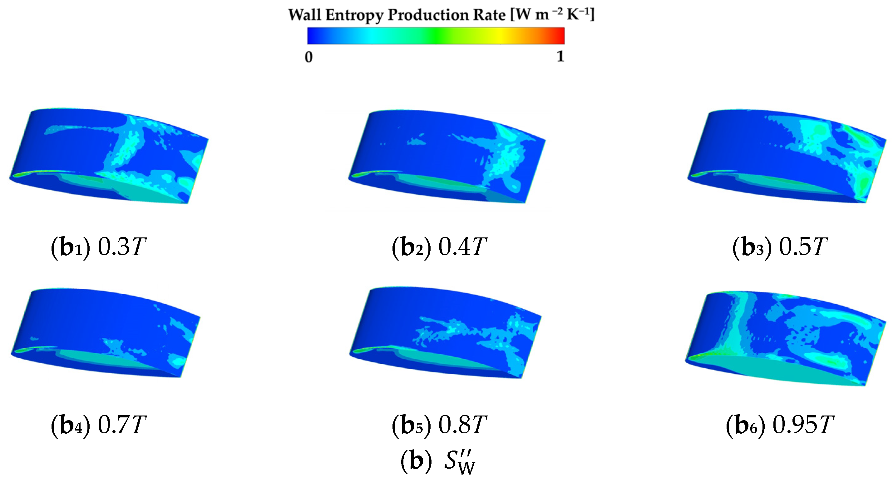
3.2. Energy Analysis

To analyze the interaction between cavity evolution and $S_{\mathrm{t}\mathrm{o}\mathrm{t}\mathrm{a}\mathrm{l}}$, Figure 6 presents the variation of $S_{\mathrm{t}\mathrm{o}\mathrm{t}\mathrm{a}\mathrm{l}}$ in a cycle.

It can be seen from Figure 6 that at 0T the cavity collapsed at the tail of the hydrofoil, which caused a strong phase transition and intense vortex movement, resulting in a higher $S_{\mathrm{t}\mathrm{o}\mathrm{t}\mathrm{a}\mathrm{l}}$. In the range of 0~0.1T, with the dissipation of the vortex in the flow field, the $S_{\mathrm{t}\mathrm{o}\mathrm{t}\mathrm{a}\mathrm{l}}$ decreased continuously. At 0.1T~0.3T, the flow pattern of the flow field was relatively stable. As the attached cavity continued to increase, the $S_{\mathrm{t}\mathrm{o}\mathrm{t}\mathrm{a}\mathrm{l}}$ increased slowly. The period of 0.4T~0.9T was the stage of attached cavity fracture and cloud cavity shedding. Due to the coupling motion of cloud cavity and vortex, the $S_{\mathrm{t}\mathrm{o}\mathrm{t}\mathrm{a}\mathrm{l}}$ increased greatly. During the period of 0.9T~1T, the $S_{\mathrm{t}\mathrm{o}\mathrm{t}\mathrm{a}\mathrm{l}}$ decreased with the collapse of the large cavity at the trailing edge of the hydrofoil. Meanwhile, a small attached cavity reappeared at the leading edge of the hydrofoil, and the variation of the $S_{\mathrm{t}\mathrm{o}\mathrm{t}\mathrm{a}\mathrm{l}}$ entered the next cycle.

The $S_{\mathrm{t}\mathrm{o}\mathrm{t}\mathrm{a}\mathrm{l}}$ within a cycle, as well as the lift and drag coefficients of the hydrofoil, are shown in Figure 7.

Figure 7 shows that in the range of 0T to 0.15T, the low-pressure region on the upper surface of the hydrofoil gradually expanded, resulting in an increase in the lift coefficient. Simultaneously, the energy loss of the flow field dropped sharply, which indicates that the vortex structure remaining in the last cycle gradually dissipated. At 0.5T~0.9T, the cloud cavity was cut off by the re-entrant jet, then fell off, moved downstream and collapsed, and the irreversible loss increased. Simultaneously, the turbulence in the cavitation flow field intensified, leading to more complicated vortex evolution. This complex evolution of the cavity led to oscillations in the lift and drag coefficients of the hydrofoil.

To quantitatively analyze the different types of entropy production value, the entropy production value of each item in a cycle is shown in Figure 8.

From Figure 8, it can be observed that the $S_{{\mathrm{D}}^{\prime }}$ was the main factor in the energy consumption, accounting for over 80%. The remaining terms, in descending order, are $S_{\overline{\mathrm{D}}}$, $S_{\mathrm{W}}$, and $S_{\mathrm{C}}$. A negative value of $S_{\mathrm{C}}$ indicates that the phase transition process is an entropy reduction process. At 0~0.1T, small-scale vortices in the wake region of the hydrofoil continued to dissipate, and the $S_{{\mathrm{D}}^{\prime }}$ decreased continuously. The $S_{\overline{\mathrm{D}}}$ also slightly decreased. Between 0.1T and 0.2T, the flow field was in a relatively stable state, the $S_{\mathrm{t}\mathrm{o}\mathrm{t}\mathrm{a}\mathrm{l}}$ was almost equal, and the $S_{\mathrm{C}}$ decreased. In addition, because of the small amount of friction between the cavity and the hydrofoil surface, the friction loss was low, resulting in a decrease in the $S_{\mathrm{W}}$. In the range of 0.4T~0.7T, as the attached cavity broke and moved downstream, the loss of the flow field was increased, lead to an increase in the $S_{\mathrm{t}\mathrm{o}\mathrm{t}\mathrm{a}\mathrm{l}}$. At 0.7T~0.9T, with the collapse of cloud cavity, the $S_{{\mathrm{D}}^{\prime }}$ continued to increase. In addition, due to the retraction of the attached cavity, the $S_{\mathrm{W}}$ increased. With the growth of the attached cavity and the dissipation of the tail vortex, the $S_{{\mathrm{D}}^{\prime }}$ dropped sharply, the $S_{\mathrm{W}}$ also decreased, and the $S_{\mathrm{t}\mathrm{o}\mathrm{t}\mathrm{a}\mathrm{l}}$ decreased.

To analyze the relationship between the dynamics of cavity detachment and the distribution of the $S_{\mathrm{t}\mathrm{o}\mathrm{t}\mathrm{a}\mathrm{l}}^{‴}$, Figure 9 demonstrates the vapor volume fraction and the $S_{\mathrm{t}\mathrm{o}\mathrm{t}\mathrm{a}\mathrm{l}}^{‴}$ at a cross-section of the hydrofoil. The shape of the cavity is represented by an iso-surface with the volume fraction of α_v = 0.1.

From Figure 9, it can be observed that in the attached cavity, the volume fraction was high, but the $S_{\mathrm{t}\mathrm{o}\mathrm{t}\mathrm{a}\mathrm{l}}^{‴}$ was relatively low. In the cloudy cavity, both the vapor fraction volume and the $S_{\mathrm{t}\mathrm{o}\mathrm{t}\mathrm{a}\mathrm{l}}^{‴}$ were high. The $S_{\mathrm{t}\mathrm{o}\mathrm{t}\mathrm{a}\mathrm{l}}^{‴}$ was predominantly concentrated at the forefront of the hydrofoil, the rear boundary of the attached cavity, the interior of the cloud cavity, and the wake region of the hydrofoil. Moreover, there consistently existed a high $S_{\mathrm{t}\mathrm{o}\mathrm{t}\mathrm{a}\mathrm{l}}^{‴}$ at the forefront of the hydrofoil throughout its cycle. Additionally, the rupture of the attached cavity also resulted in a significant $S_{\mathrm{t}\mathrm{o}\mathrm{t}\mathrm{a}\mathrm{l}}^{‴}$ in the rupture zone.

For a deeper analysis of the characteristics of various entropy production rates and their interrelationships with cavity shape, Figure 10 illustrates the evolution process of the cavity shape (α_v = 0.1), the $S_{\overline{\mathrm{D}}}^{‴}$, as well as the $S_{D^{\prime }}^{‴}$ at a cross-section of the hydrofoil within a cycle.

Figure 10a indicates that the $S_{\overline{\mathrm{D}}}^{‴}$ was mainly concentrated near the stagnation point of the hydrofoil and the inner region of the cavity. Near the stagnation point, the fluid separated, and then the flow direction changed, resulting in the generation of unsteady vortices. In the cavity, due to the mixing of vapor and liquid phases, some energy loss was also caused. Figure 10b reveals that the higher $S_{D^{\prime }}^{‴}$ mainly occured in the fluid domain below the lifted attached cavity and inside the vortex induced by the cloud cavity. The reason is that the re-entrant jet collided with the main stream, resulting in strong vortices, which increased the $S_{D^{\prime }}^{‴}$. The distribution of the $S_{D^{\prime }}^{‴}$ was similar to that of the $S_{\mathrm{t}\mathrm{o}\mathrm{t}\mathrm{a}\mathrm{l}}^{‴}$, indicating that the energy loss of the hydrofoil cavitation flow field was mainly composed of turbulent dissipation.

For analyzing the relationship between the cavity shape and $S_{\mathrm{C}}^{‴}$, Figure 11 presents the cavity shape (α_v = 0.1), the $S_{\mathrm{C}}^{‴}$, and the $\dot{m}$ at a cross-section of the hydrofoil in a cycle. In the $\dot{m}$ distribution, the negative value represents the condensation process and the positive value represents the evaporation process.

From Figure 11a, it can be observed that a high $S_{\mathrm{C}}^{‴}$ was primarily concentrated at the vapor–liquid interface, which is consistent with the view that the $S_{\mathrm{C}}^{‴}$ mainly comes from the mass exchange between the two phases. Figure 11b indicates that the evaporation rate inside the cavity and the condensation rate at the edge of the cavity were relatively high. Between the regions of high evaporation and high condensation rates, there existed a transition zone with low $\dot{m}$. In this region, the $S_{\mathrm{C}}^{‴}$ was relatively low.

In order to analyze the relationship between the vapor volume fraction and the $S_{\mathrm{W}}^{″}$ distribution, Figure 12 demonstrates the changing process of the vapor volume fraction and the $S_{\mathrm{W}}^{″}$ on the hydrofoil surface. The shape of the cavity was selected as the iso-surface with volume fraction α_v = 0.1.

Figure 12 reveals that in the whole period, the high $S_{\mathrm{W}}^{″}$ was mainly concentrated in the area where the cavity is not covered. The reason is that near the viscous bottom layer of the hydrofoil, the shear stress between the water and wall is larger than that between the cavity and wall, and the velocity of water is larger than the mixture in the cavity, so the energy loss of the hydrofoil surface which is not covered by the cavity is larger.

4. Conclusions

In order to gain a more comprehensive understanding of the energy loss caused by cavitation, this article used a k-ε model (modified with FBDCM) and ZGB cavitation model to numerically simulate the cavitation flow field around a 3-dimensional NACA66 hydrofoil. The main summaries are as follows:

(1)

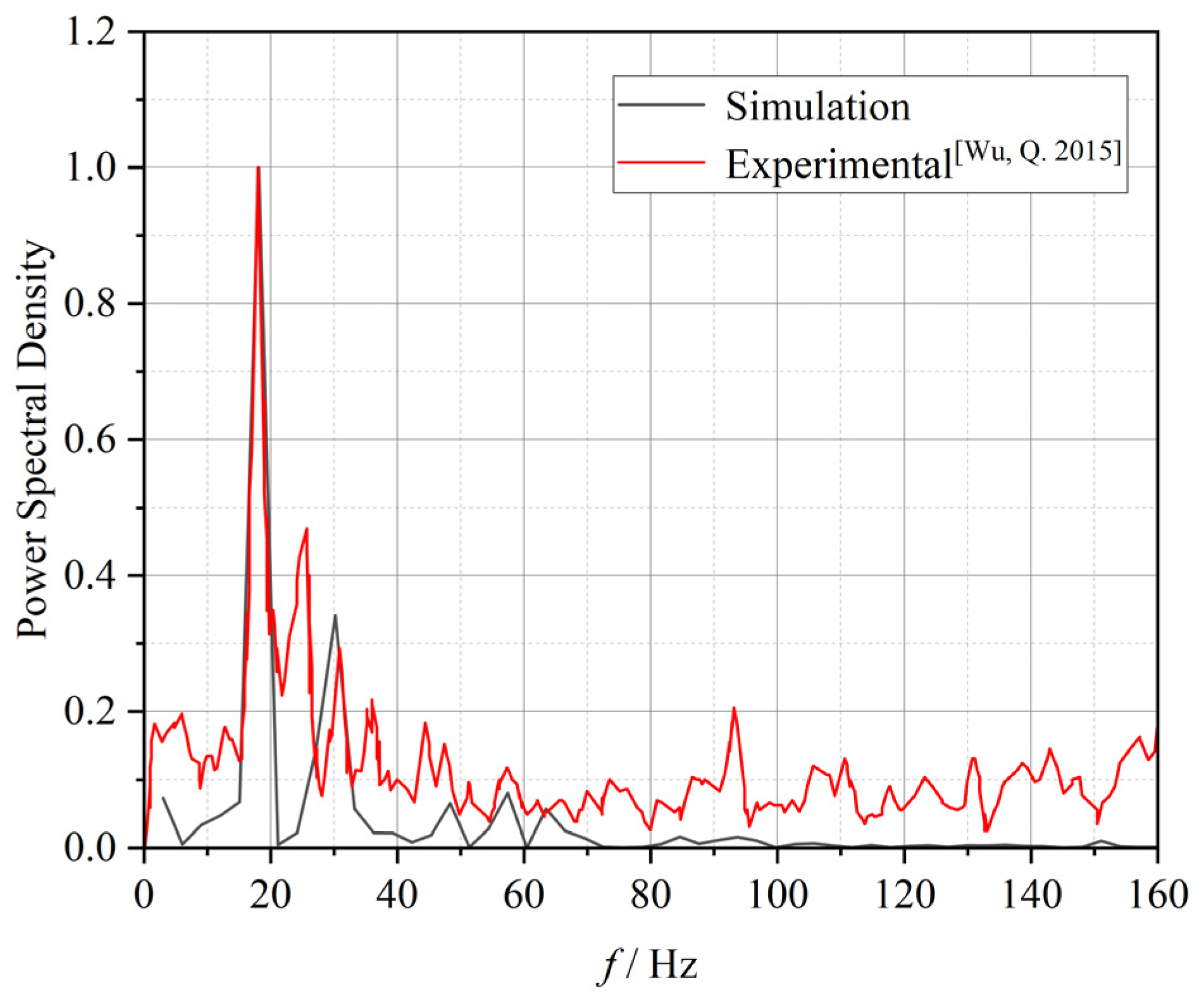
According to the comparison with the experiment results, FBDCM can effectively capture the flow characteristics of cavity initiation, development, fracture, shedding, and collapse, revealing the complex dynamics between cavitation and vortexes. The numerical model in this paper can accurately predict the lift coefficient, drag coefficient, and the frequency of cavitation evolution.

(2)

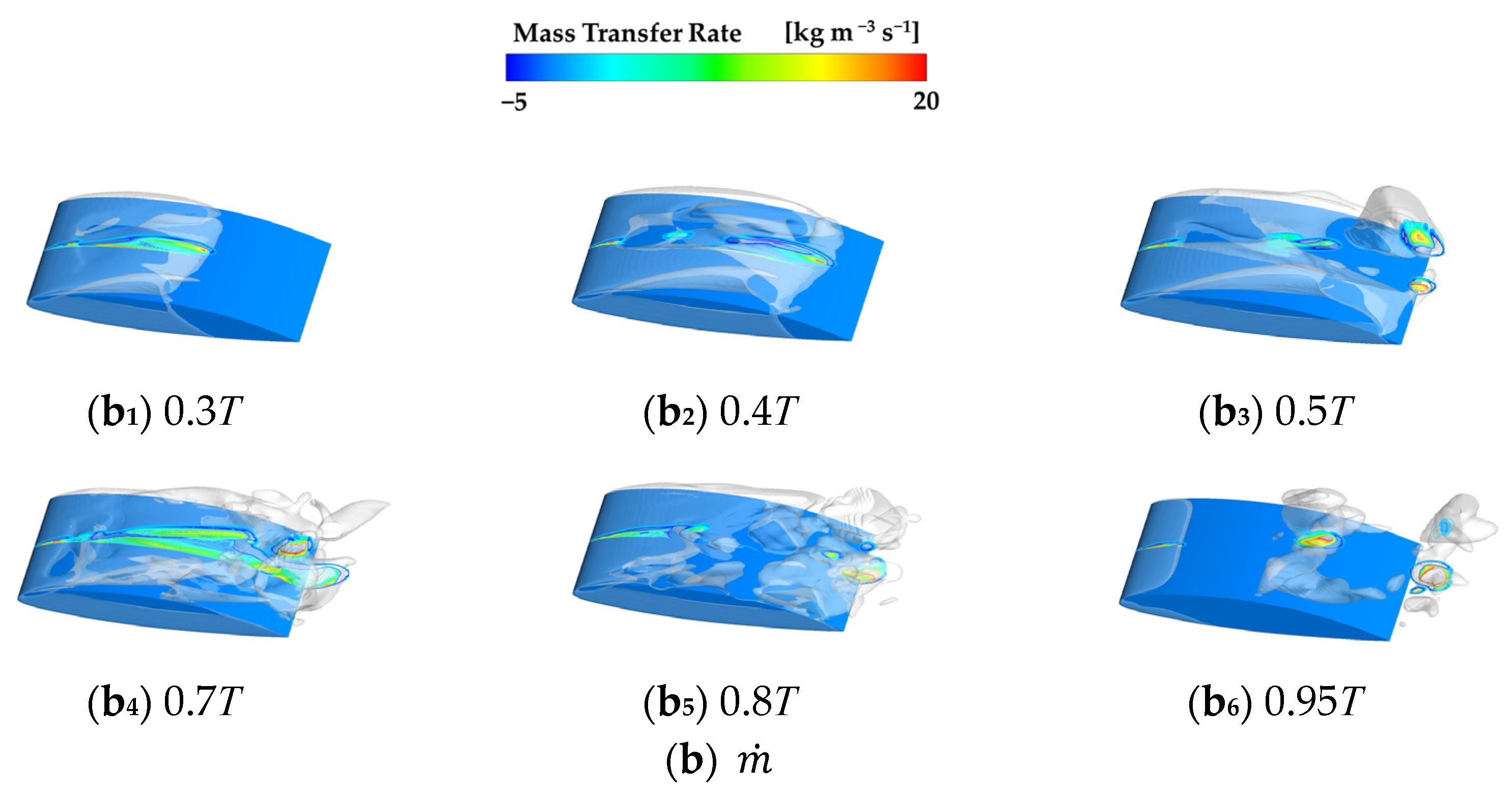
The vortex dilatation term in the vorticity transport equation plays a crucial role throughout the cavitation evolution cycle. The impact of the vortex stretching term on vorticity transport is slightly greater than that of the baroclinic torque term. The vortex stretching term mainly exists on the right cavity surface of the hydrofoil and the left leakage cavity surface. In 0.3T~0.4T (cavity growing stage), the vortex dilatation term promotes the development of cavity. In 0.5T~0.8T (cavity shedding stage), the volume of the cloud cavity continues to increase, the vortex expansion ability inside the cavity weakens, and the ability of the vortex dilatation term to transport vortices decreases. The baroclinic moment term has a weak impact on the whole cavity evolution process, primarily appearing at the boundary of the cavity closure region.

(3)

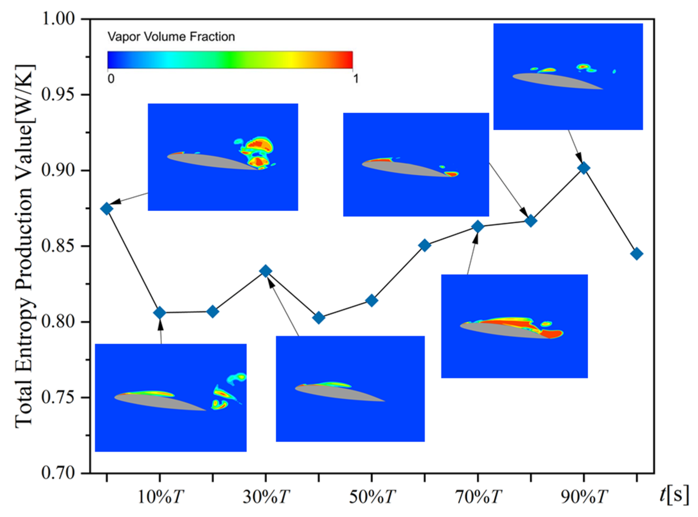
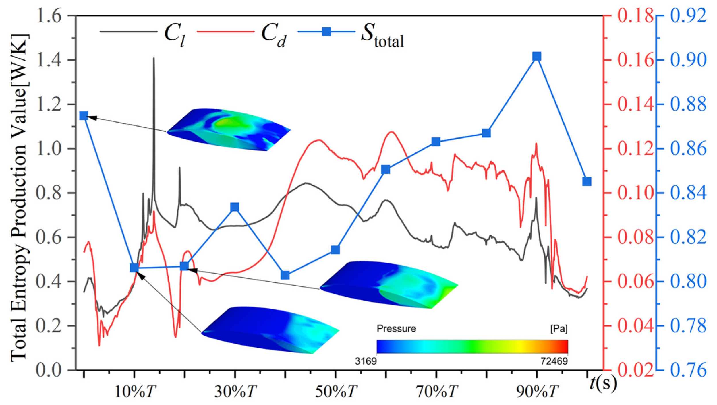
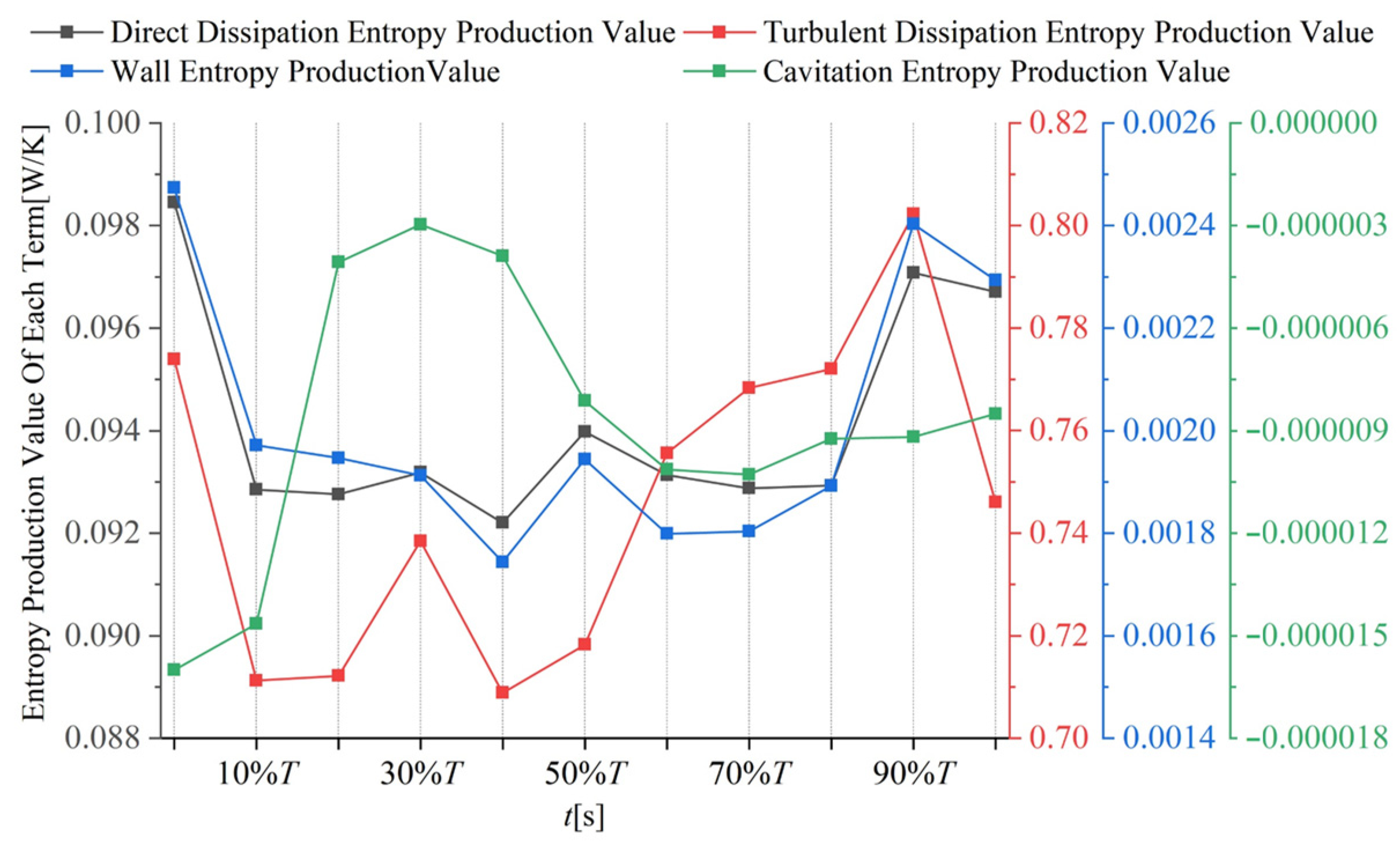
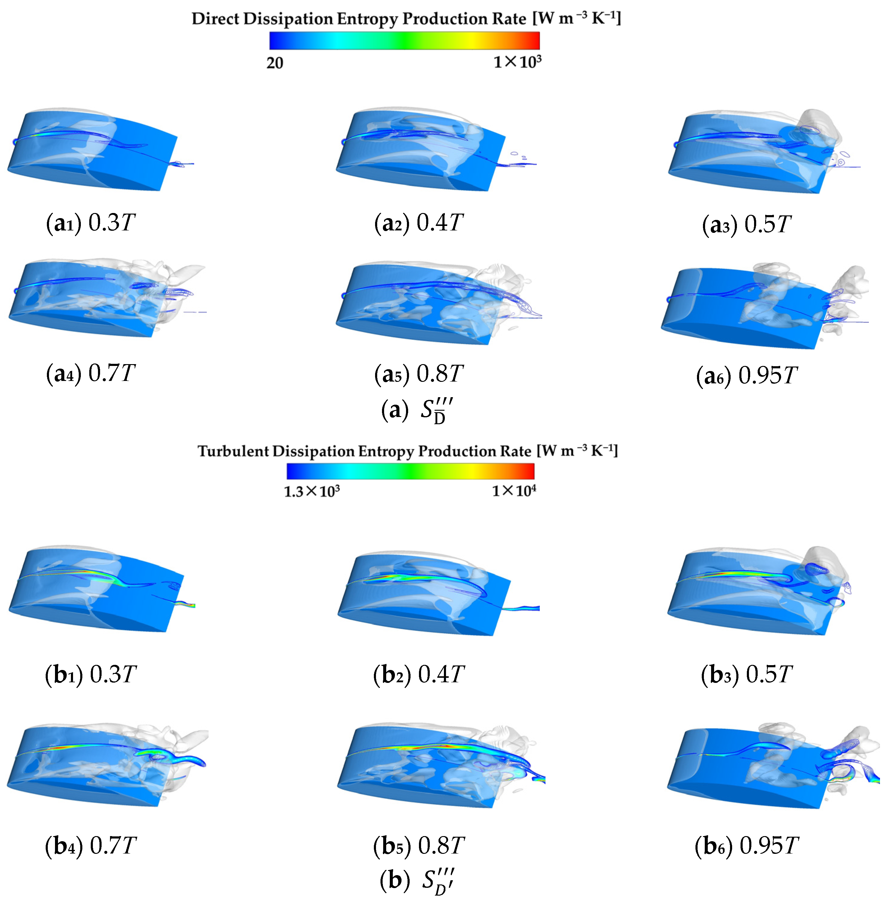
During the phenomenon of cloud cavity shedding and collapse, the total entropy production value in the flow field is significant. When the cavity collapses, the total entropy production value reaches its peak value. The turbulent dissipation entropy production rate is predominantly localized in the fluid domain below the lifted attached cavity and within the vortex induced by the cloud cavity, accounting for over 80% of the total entropy production. The direct dissipation entropy production rate primarily occurs near the stagnation point of the hydrofoil’s leading edge and inside the cavity. The wall entropy production rate is concentrated in uncovered cavity areas, while the cavitation entropy production rate is mainly concentrated on the vapor–liquid interface.

This paper has established a suitable numerical model for simulating cavitation flow around the NACA66 hydrofoil and has obtained the detailed relationship between the entropy production rate distribution and flow structure. The conclusions drawn in this article can be applied to hydrofoil design to reduce cavitation and energy loss. However, there are still some studies that have not been thoroughly conducted, and the research conditions should be further expanded, such as different angles of attack, Reynolds numbers, cavitation numbers, temperatures, and other parameters. This is also the author’s further work.

References

1. Kollek, W.; Kudźma, Z.; Stosiak, M.; Mackiewicz, J. Possibilities of diagnosing cavitation in hydraulic systems. Arch. Civ. Mech. Eng. 2007, 7, 61–73. [Google Scholar] [CrossRef]
2. Liu, Y.; Li, X.; Wang, W.; Li, L.; Huo, Y. Numerical investigation on the evolution of cavitating dynamics and energy loss around a hydrofoil in fluoroketone under different temperatures. Ocean Eng. 2023, 287, 115856. [Google Scholar] [CrossRef]
3. Karpenko, M. Aircraft hydraulic drive energy losses and operation delay associated with the pipeline and fitting connections. Aviation 2024, 28, 1–8. [Google Scholar] [CrossRef]
4. Bejan, A.; Kestin, J. Entropy Generation through Heatand Fluid Flow; John Wiley & Sons Inc.: New York, NY, USA, 1982. [Google Scholar] [CrossRef]
5. Kock, F.; Herwig, H. Local entropy production in turbulent shear flows: A high-Reynolds number model with wall functions. Int. J. Heat Mass Transf. 2003, 47, 2205–2215. [Google Scholar] [CrossRef]
6. Wang, W.; Wang, J.; Li, J.; Liang, Z. Entropy generation rates calculation in turbulent flow through an airfoil based on eddy viscosity models. Chin. J. Comput. Mech. 2018, 35, 387–392. [Google Scholar] [CrossRef]
7. Zhang, Y.; Yang, B.; Chen, W.; Chen, H.; Xiang, L. Study on Cavitation Characteristics of Hydrofoil Based on Entropy Production Theory. J. Propuls. Technol. 2019, 40, 1490–1497. [Google Scholar] [CrossRef]
8. Yu, A.; Tang, Q.; Zhou, D. Entropy production analysis in thermodynamic cavitating flow with the consideration of local compressibility. Int. J. Heat Mass Transf. 2020, 153, 119604. [Google Scholar] [CrossRef]
9. Gu, Y.; Qiu, Q.; Ren, Y.; Ma, L.; Ding, H.; Hu, C.; Wu, D.; Mou, J. Cavitation flow of hydrofoil surface and turbulence model applicability analysis. Int. J. Mech. Sci. 2024, 277, 109515. [Google Scholar] [CrossRef]
10. He, Z.; Guan, W.; Wang, C.; Guo, G.; Zhang, L.; Gavaises, M. Assessment of turbulence and cavitation models in prediction of vortex induced cavitating flow in fuel injector nozzles. Int. J. Multiph. Flow 2022, 157, 104251. [Google Scholar] [CrossRef]
11. Johansen, S.T.; Wu, J.; Shyy, W. Filter-based unsteady RANS computations. Int. J. Heat Fluid Flow 2003, 25, 10–21. [Google Scholar] [CrossRef]
12. Coutier-Delghosa, O.; Fortes-Patella, R.; Reboud, J.L. Evaluation of the Turbulence Model Influence on the Numerical Sim-ulations of Unsteady Cavitation. J. Fluids Eng. 2003, 125, 38–45. [Google Scholar] [CrossRef]
13. Liu, J.; Yu, J.; Yang, Z.; He, Z.; Yuan, K.; Guo, Y.; Li, Y. Numerical investigation of shedding dynamics of cloud cavitation around 3D hydrofoil using different turbulence models. Eur. J. Mech. B/Fluids 2021, 85, 232–244. [Google Scholar] [CrossRef]
14. Yin, T.; Pavesi, G.; Pei, J.; Yuan, S. Numerical analysis of unsteady cloud cavitating flow around a 3D Clark-Y hydrofoil considering end-wall effects. Ocean Eng. 2021, 219, 108369. [Google Scholar] [CrossRef]
15. Huang, B.; Wang, G.; Zhao, Y. Numerical simulation unsteady cloud cavitating flow with a filter-based density correction model. J. Hydrodyn. 2014, 26, 26–36. [Google Scholar] [CrossRef]
16. Huang, B.; Wang, G.; Yuan, H.; Wang, F. Assessment of a Density Modify Based Turbulence Closure for Unsteady Cavitating Flows. Trans. Beijing Inst. Technol. 2010, 30, 1170–1174. [Google Scholar] [CrossRef]
17. Suarez, S.; Puyol, R.; Schafer, C.; Mucklich, F. Numerical investigation of dynamics of unsteady sheet/cloud cavitating flow using a compressible fluid model. Mod. Phys. Lett. B 2015, 29, 1450269. [Google Scholar] [CrossRef]
18. Zwart, P.J.; Gerber, A.G.; Belamri, T. A two-phase flow model for predicting cavitation dynamics. In Proceedings of the 5th International Conference on Multiphase Flow, Yokohama, Japan, 30 May–4 June 2004. [Google Scholar]
19. Suarez, S.; Puyol, R.; Schafer, C.; Mucklich, F. Lift-drag characteristics of S-shaped hydrofoil under different cloud cavitation conditions. Ocean Eng. 2023, 278, 114374. [Google Scholar] [CrossRef]
20. Suarez, S.; Puyol, R.; Schafer, C.; Mucklich, F. Thermodynamic effect on attached cavitation and cavitation-turbulence interaction around a hydrofoil. Ocean Eng. 2023, 281, 114764. [Google Scholar] [CrossRef]
21. Suarez, S.; Puyol, R.; Schafer, C.; Mucklich, F. Numerical Prediction of Cavitating Flow on a Two-Dimensional Symmetrical Hydrofoil and Comparison to Experiments. J. Fluids Eng. 2007, 129, 279–292. [Google Scholar] [CrossRef]
22. Yu, A.; Li, L.; Zhou, D.; Ji, J. Large eddy simulation of the pulsation characteristics in the cavitating flow around a NACA0015 hydrofoil. Ocean Eng. 2023, 267, 113289. [Google Scholar] [CrossRef]
23. Liu, Y.; Li, X.; Ge, M.; Li, L.; Zhu, Z. Numerical investigation of transient liquid nitrogen cavitating flows with special emphasis on force evolution and entropy features. Cryogenics 2021, 113, 103225. [Google Scholar] [CrossRef]
24. Kock, F.; Herwig, H. Entropy production calculation for turbulent shear flows and their implementation in cfd codes. Int. J. Heat Fluid Flow 2005, 26, 672–680. [Google Scholar] [CrossRef]
25. Zhang, X.; Wang, Y.; Xu, X.; Wang, H. Energy Conversion Characteristic within Impeller of Low Specific Speed Centrifugal Pump. Nongye Jixie Xuebao 2011, 42, 75–81. [Google Scholar] [CrossRef]
26. Wu, Q.; Huang, B.; Wang, G.; Gao, Y. Experimental and numerical investigation of hydroelastic response of a flexible hydrofoil in cavitating flow. Int. J. Multiph. Flow 2015, 74, 19–33. [Google Scholar] [CrossRef]
Figure 1. Three-dimensional computational domain of the hydrofoil.
Processes 12 01780 g001
Figure 2. The mesh details of the hydrofoil surface.
Processes 12 01780 g002
Figure 3. The normalized power spectral density of the lift coefficient between the numerical simulation and experimental results [26].
Processes 12 01780 g003
Figure 4. The experimental results [26], vortex structure evolution (iso−surface of Q = 2 × 10⁵ s−2), and cavity shape (αv = 0.1) in a cycle.
Processes 12 01780 g004
Figure 5. The evolution of the vorticity, RVS, RVD, and BT in a cycle.
Processes 12 01780 g005aProcesses 12 01780 g005b
Figure 6. The variation of S t o t a l in a cycle.
Processes 12 01780 g006
Figure 7. Lift coefficient, drag coefficient, and S t o t a l in a cycle.
Processes 12 01780 g007
Figure 8. The entropy production value of each item in a cycle.
Processes 12 01780 g008
Figure 9. The vapor volume fraction and the S t o t a l on the middle cross plane of the hydrofoil in a cycle.
Processes 12 01780 g009aProcesses 12 01780 g009b
Figure 10. The S D ¯ and the S D on the middle cross plane of the hydrofoil in a cycle.
Processes 12 01780 g010
Figure 11. The S C and the m ˙ on the middle cross plane of the hydrofoil in a cycle.
Processes 12 01780 g011aProcesses 12 01780 g011b
Figure 12. Vapor volume fraction and wall entropy production rate on the hydrofoil surface.
Processes 12 01780 g012aProcesses 12 01780 g012b