Pour Point Prediction Method for Mixed Crude Oil Based on Ensemble Machine Learning Models

Abstract

Pipelines are the most common way to transport crude oil. The crude oil developed from different fields is mixed first and then transported. The pour point of mixed crude oil is very important for pipeline schemes and ensuring the safe, efficient, and flexible operation of the pipeline. An integrated machine learning model based on XGBoost is identified as optimal to predict the pour point of mixed crude oil by comprehensive comparison among six different types of machine learning models: multiple linear regression, random forest, support vector machine, LightGBM, backpropagation neural network, and XGBoost. A mixed crude oil pour point prediction model with strong engineering adaptability is proposed, focusing on enhancing the flexibility of machine learning model inputs (using density and viscosity instead of component crude oil pour points) and addressing challenges such as data volume and input missing in engineering scenarios. With the inputs of pour point T_g, density ρ, viscosity μ, and ratio X_i in component oils, the mean absolute error of the model prediction estimations after training with 8912 data is 1.12 °C, when the pour point T_g of the component crude oil is missing, the mean absolute error is 1.93 °C and the percentage of the predicted absolute error within 2 °C is 88.0%. This study can provide support for the intelligent control of flow properties of pipeline transport mixed oil.

1. Introduction

Pipelines are the most common way to transport crude oil. The crude oil developed from different fields is mixed first and then transported. The online monitoring of crude oil properties and the real-time prediction of mixed crude oil properties is necessary for the intelligent, safe, and efficient operation of mixed crude oil transportation pipelines. The pour point of crude oil has an important impact on temperature control, transportation method selection, and the safe and efficient operation of a crude oil pipeline. Presently, the pour point of mixed crude oil entering pipelines is monitored through manual sampling. Manual sampling testing is inefficient, leading to delays in obtaining pour point measurements for mixed crude oil. The crude oil properties cannot be obtained in a timely and effective manner during transportation, because the measurement of the pour point occurs after the mixed crude oil enters the pipeline.

The pour point is influenced by the interaction of various crude oil components (e.g., wax, colloids, asphaltenes, and light hydrocarbons), resulting in a nonlinear relationship between the pour point of mixed crude oil and that of component crude oils, lacking a reliable theoretical model [1]. The crude oil transported via long-distance pipelines may originate from multiple sources, with properties varying significantly across different blocks of the same oil field, causing substantial fluctuations in the properties of “the same type of oil” [2]. Hence, the prediction of the pour point of mixed crude oil is full of challenges. At present, the pour point prediction for mixed crude oil is mainly achieved by the empirical model and the machine learning model.

The empirical model for calculating the mixed crude oil pour point is based on the component crude oil pour points and their proportion [3]. The relationship between the pour point of mixed crude oil and that of the component crude oil does not follow linear weighted rules [4] (i.e., Equation (1)). Consequently, researchers have endeavored to refine this relationship. Notable efforts include the model proposed by Liu et al. (i.e., Equation (2)) [5] and Li et al. (i.e., Equation (3)) [6]. These models introduce two correction coefficients—one for the blending ratio of mixed crude oil and another for the pour point of a 1:1 mixture of two component oils. Such adjustments significantly enhance the accuracy of mixed crude oil pour point calculation [7]. However, the inclusion of pour points for equally proportioned mixed crude oil constrains the practicality of these models due to the demanding usage condition, particularly for multi-component mixed crude oil. In scenarios where component crude oil properties exhibit significant fluctuations, the utility of these models becomes challenging. Moreover, owing to the strong sensitivity of pour points to conditions and the inherent limitation of the measurement method, the accuracy of crude oil pour point determination is restricted (testing specifications typically demand a repeatability of 2 °C). Consequently, these empirical models lack robustness against data noise.

To address the stringent applicability conditions arising from the need for equally proportioned mixed crude oils, Chen et al. [7] conducted extensive analysis on mixed crude oil pour point data. They discovered a strong correlation between the absolute deviations of pour points calculated using linear weighted methods for equally proportioned mixed crude oils and the absolute difference between the pour points of two component oils, leading to the formulation of Equation (4). Similarly, Loskutova and Yudina [8], and Majhi et al. [9] utilized pour point data from 76 equally proportioned mixtures of two component crude oils to develop mixed crude oil pour point calculation models (Equations (5) and (6)) that do not rely on equally proportioned data for two component crude oils. However, while eliminating the dependence on pour points of equally proportioned mixed crude oils, these models suffer from reduced prediction accuracy. Summary information of empirical models is presented in

Table 1. Summary of empirical models for pour point of mixed crude oil prediction.

Empirical Model Formulation for Pour Point Prediction	Number	References
$T_{\mathrm{gm}}={\displaystyle \sum _{i=1}^N\left(X_i,T_{\mathrm{g}i}\right)}$	(1)	[4]
$\left\{\begin{array}{l}{T}_{\mathrm{gm}}={\displaystyle \sum _{i=1}^N\left(X_i,T_{\mathrm{g}i}\right)}+{\displaystyle \sum _{j=1}^{N-1}{\displaystyle \sum _{k=j+1}^N\left(B_{jk}\cdot C_{jk}\cdot X_j\cdot X_k\right)}}\\ B_{jk}=1-{\displaystyle \frac{X_k}{2}}+{\displaystyle \frac{X_j}{2}},\begin{array}{cc}& T_{\mathrm{g}k}>T_{\mathrm{g}j}\end{array}\\ C_{jk}=2\left(2T_{\mathrm{g}jk}-T_{\mathrm{g}j}-T_{\mathrm{g}k}\right)\end{array}\right.$	(2)	[5]
$\left\{\begin{array}{l}{T}_{\mathrm{g}m}={\displaystyle \sum _{i=1}^N\left(X_i,T_{\mathrm{g}i}\right)}+{\displaystyle \sum _{j=1}^{N-1}{\displaystyle \sum _{k=j+1}^N\left(B_{jk}\cdot C_{jk}\cdot X_j\cdot X_k\right)}}\\ B_{jk}={\left[{\displaystyle \frac{\lg \left(100X_j\right)}{\lg \left(100X_k\right)}}\right]}^{\mathrm{sign}\left(C_{jk}\right)},\begin{array}{cc}& T_{\mathrm{g}k}>T_{\mathrm{g}j}\end{array}\\ C_{jk}=2\left(2T_{\mathrm{g}jk}-T_{\mathrm{g}j}-T_{\mathrm{g}k}\right)\end{array}\right.$	(3)	[6]
$\left\{\begin{array}{l}{T}_{\mathrm{gm}}={\displaystyle \sum _{i=1}^N\left(X_i,T_{\mathrm{g}i}\right)}+{\displaystyle \sum _{j=1}^{N-1}{\displaystyle \sum _{k=j+1}^N\left(B_{jk}\cdot C_{jk}\cdot X_j\cdot X_k\right)}}\\ B_{jk}=1-{\displaystyle \frac{X_k}{2}}+{\displaystyle \frac{X_j}{2}},\begin{array}{cc}& T_{\mathrm{g}k}>T_{\mathrm{g}j}\end{array}\\ C_{jk}=\pm 0.698\left|T_{\mathrm{g}j}-T_{\mathrm{g}k}\right|\end{array}\right.$	(4)	[7]
$\left\{\begin{array}{l}{T}_{\mathrm{gm}}={\displaystyle \sum _{i=1}^N\left(X_i,T_{\mathrm{g}i}\right)}+{\displaystyle \sum _{j=1}^{N-1}{\displaystyle \sum _{k=j+1}^N\left(B_{jk}\cdot C_{jk}\cdot X_j\cdot X_k\right)}}\\ B_{jk}=1-{\displaystyle \frac{X_k}{2}}+{\displaystyle \frac{X_j}{2}},\begin{array}{cc}& T_{\mathrm{g}k}>T_{\mathrm{g}j}\end{array}\\ C_{jk}=0.2904{\left(T_{\mathrm{g}j}-T_{\mathrm{g}k}\right)}^{1.349}\end{array}\right.$	(5)	[8]
$\left\{\begin{array}{l}{T}_{\mathrm{gm}}={\displaystyle \sum _{i=1}^N\left(X_i,T_{\mathrm{g}i}\right)}+{\displaystyle \sum _{j=1}^{N-1}{\displaystyle \sum _{k=j+1}^N\left(B_{jk}\cdot C_{jk}\cdot X_j\cdot X_k\right)}}\\ B_{j,k}=1-{\displaystyle \frac{X_k}{2}}+{\displaystyle \frac{X_j}{2}},\begin{array}{cc}& T_{\mathrm{g}k}>T_{\mathrm{g}j}\end{array}\\ C_{j,k}=0.59{\left(T_{\mathrm{g}j}-T_{\mathrm{g}k}\right)}^{1.1394}\end{array}\right.$	(6)	[9]

, where $T_{gm}$ represents the pour point of mixed crude oil, $T_{gi}$ denotes the pour point of component crude oil $i$, $X_i$ signifies the proportion of component crude oil $i$, $T_{gjk}$ indicates the pour point of a mixture of component crude oils $j$ and $k$ with equal proportions, and $B_{jk}$ and $C_{jk}$ are correction coefficients. Based on the aforementioned considerations, the essential input parameters for predicting the pour point of blended crude oil include the blend ratio of the mixed crude oil and the pour point of the component oils. Empirical models with superior prediction accuracy (Equations (2) and (3)) necessitate knowledge of the pour point of the blended crude oil. Consequently, other physical parameters capable of partially characterizing crude oil, such as density and viscosity, have yet to be incorporated into the prediction of the pour point of blended crude oil.

Although the empirical model for calculating mixed crude oil pour points is practical, improving its prediction accuracy remains a challenge. With the rapid advancement of machine learning algorithms, leveraging measured data to establish machine learning models for understanding pour point patterns in multi-component mixed crude oil offers a promising avenue for enhancing prediction accuracy. In comparison to empirical models that derive mathematical equations through fitting, machine learning exhibits superior capabilities in uncovering implicit data patterns and possesses dynamic adaptive capabilities. Hou et al. [10] developed a mixed crude oil pour point prediction model based on fully connected neural networks trained using back propagation. Leveraging experimental and literature-derived data, component crude oil pour points and proportions were input parameters, while the resulting mixed crude oil pour point served as the output parameter. The model outperformed empirical models in predictive performance. However, the training sample size comprised 357 sets (with data before and after crude oil mixing considered as one set), and the validation sample size was 36 sets. Analysis of the resistance of established machine learning models to data noise was not provided. Furthermore, recent advancements in machine learning algorithms warrant the application of more powerful algorithms in mixed crude oil pour point prediction.

This paper reviews empirical models for mixed crude oil pour point prediction as a benchmark for assessing the effectiveness of machine learning models. By comparing various machine learning models for pour point prediction of different mixed crude oil types, a mixed crude oil pour point prediction model based on the XGBoost ensemble machine learning algorithm is identified as optimal. Building upon this, a mixed crude oil pour point prediction model with strong engineering adaptability is proposed, focusing on enhancing the flexibility of machine learning model inputs (using density and viscosity instead of component crude oil pour points) and addressing challenges such as data volume and input missing in engineering scenarios. Leveraging the powerful data mining capabilities of machine learning models can address the issue of online prediction of pour points for blended crude oils in the presence of missing data (such as pour points of component crude oils) encountered in production. Empirical models exhibit less sensitivity to the amount of fitting data, while machine learning models are more sensitive. Therefore, in situations with limited data, empirical models can be used for prediction. As the amount of data increases, a combination of empirical and machine learning models can be employed, transitioning ultimately to machine learning models.

2. Prediction Model

The lack of reliable technology for online pour point monitoring impedes real-time online prediction of mixed crude oil pour points. Characterizing crude oil, especially mixed crude oil, based on typical properties (pour point, viscosity, and density) and their nonlinear relationships could provide insights. Combining machine learning models with online monitoring of other crude oil properties (e.g., density and viscosity) holds potential for achieving online pour point prediction and control during pipeline transportation. Nonetheless, research on modeling the relationship between different properties of mixed crude oil remains scarce.

2.1. Ensemble Learning Algorithms

Ensemble learning represents a prevailing trend in contemporary machine learning algorithms. Its fundamental concept involves sampling multiple subsets from the overall dataset, constructing sub-models based on these subsets, and effectively amalgamating multiple sub-learners to form an ensemble learner exhibiting notably enhanced accuracy and generalization compared to an individual learner. This approach serves to mitigate the inherent risk of under fitting in single learners, thereby achieving heightened stability and predictive efficacy [11]. Machine learning models operating within the ensemble learning framework boast advantages such as robust nonlinear fitting capabilities, resilience to noise, and computational efficiency [12]. These attributes offer substantial support for modeling the intricate relationships among the diverse properties of crude oil. Consequently, this study integrates ensemble machine learning methodologies for predicting the pour point of blended crude oil. The evolution of input–output relationships for each model forecasting the pour point of blended crude oil is depicted in Figure 1.

Ensemble machine learning models are commonly based on tree models, forming two typical branches of ensemble models by integrating different ensemble principles with tree models [13]. When combined with the bagging strategy, tree models give rise to the random forest model; when combined with the boosting strategy, they yield the Gradient Boosting Decision Tree (GBDT) model [14]. The GBDT model has exhibited remarkable performance across various research domains and data competitions. However, the substantial time and cost involved in parameter training constrain the practical application of GBDT models. XGBoost (eXtreme Gradient Boosting) emerges as an efficient and flexible ensemble model. Through the incorporation of regularization terms and optimization of the second-order derivative calculation of GBDT models, XGBoost enhances the training efficiency of GBDT models while maintaining predictive performance [15]. Although LightGBM optimizes the structure based on XGBoost, it sacrifices some degree of prediction accuracy. In engineering applications for pour point prediction, models typically demand minimal training and self-optimization time. Pre-trained models can be deployed, with periodic updates based on data changes during usage [16]. Considering both model performance and training efficiency, this study adopted XGBoost for modeling the pour point prediction of blended crude oil.

The base learner in the XGBoost model is CART (Classification and Regression Tree). A single CART comprises multiple leaf nodes. Throughout the training and application phases of the model, a given set of input data corresponds to an output value at the leaf node. The collective outputs of multiple leaf nodes in a single CART represent the prediction result for the current input data [17]. Accordingly, the XGBoost model computes the sum of predicted values from all CARTs for a sample as the output value ${\widehat{y}}_i$ for that sample, as depicted in Equations (7) and (8):

$${\widehat{y}}_i=\varphi \left(x_i\right)={\displaystyle \sum _{k=1}^K{f}_k}\left(x_i\right),\hspace{1em}{f}_k\in \Gamma$$

(7)

$$\Gamma =\left\{f(x)=w_{q(x)}\right\}\left(q:R^m\to n,w\in R^n\right)$$

(8)

where ${\widehat{y}}_i$ represents the predicted value of the model for the ith sample; $x_i$ denotes the ith sample; $f_k$ denotes the $k$th tree model; $\Gamma$ represents the space of decision trees; m is the number of features; n is the number of leaf nodes for each tree; q represents the structure mapping each sample to the corresponding leaf node scores for each tree, i.e., q represents the tree model, which takes a sample as input and maps it to the leaf nodes to output prediction scores; and $w_{q\left(x\right)}$ is the set comprising the scores of all leaf nodes of tree q.

The essence of machine learning models lies in the optimization problem aimed at minimizing the statistical value of the loss function on training data. The loss function (optimization objective) for the XGBoost model is defined as follows in Equation (9):

$$\mathcal{L}(\varphi )={\displaystyle \sum _{i}l}\left({\widehat{y}}_i,y_i\right)+{\displaystyle \sum _k\Omega }\left(f_k\right)$$

(9)

$$\Omega \left(f_k\right)=\gamma n+{\displaystyle \frac{1}{2}}\lambda {\displaystyle \sum _{j=1}^n{w}_j^2}$$

(10)

n represents the number of leaf nodes within a tree; $\gamma$ denotes the regularization penalty for $L_1$, wherein a higher count of leaf nodes entails a stronger penalty; $\lambda$ signifies the squared $L_2$ norm of the scores w associated with the leaf nodes in a tree. The first term on the right-hand side of Equation (9) is the loss function term, representing the training error, and it is a differentiable convex function. The second term is the regularization penalty term, denoting the sum of complexities across all trees, aimed at controlling the model’s complexity and mitigating overfitting.

Hence, the training objective of the model shifts to minimizing $\mathcal{L}\left(\varphi \right)$ to derive the corresponding model $f_k$. As the optimization parameter in the XGBoost model is the model $f_k$, not a specific value, conventional optimization methods cannot be employed for optimization in Euclidean space. Incremental training is necessary to update the model. Each iteration retains the original model unchanged and incorporates a new function $f_t\left(x_i\right)$ into the model, as shown in Equation (11):

$$\begin{array}{l}{\widehat{y}}_i^{(0)}=0\hfill \\ {\widehat{y}}_i^{(1)}=f_1\left(x_i\right)={\widehat{y}}_i^{(0)}+f_1\left(x_i\right)\hfill \\ {\widehat{y}}_i^{(2)}=f_1\left(x_i\right)+f_2\left(x_i\right)\hfill \\ \cdots \hfill \\ {\widehat{y}}_i^{(t)}={\displaystyle \sum _{k=1}^t{f}_k}\left(x_i\right)={\widehat{y}}_i^{(t-1)}+f_t\left(x_i\right)\hfill \end{array}$$

(11)

In the context of fitting, the square error loss function based on Equation (11) is transformed into the form of Equation (12):

$${\mathcal{L}}^{(\mathrm{t})}={\displaystyle \sum _{i=1}^n{\left(y_i-\left({\widehat{y}}_i^{(t-1)}+f_t\left(x_i\right)\right)\right)}^2}+\Omega \left(f_t\right)={\displaystyle \sum _{i=1}^n\left[2\left({\widehat{y}}_i^{(t-1)}-y_i\right)f_t\left(x_i\right)+f_t{\left(x_i\right)}^2\right]}+\Omega \left(f_t\right)$$

(12)

The Taylor series approximation is applied to expand Equation (12), isolating the constant term to simplify the objective function. The Taylor expansion formula is represented as Equation (13):

$$f(x+\Delta x)\approx f(x)+f^{\prime }(x)\Delta x+{\displaystyle \frac{1}{2}}{f}^{″}(x)\Delta x^2$$

(13)

Combining with Equation (13), the expanded form of Equation (12) is represented as Equation (14):

$${\mathcal{L}}^{(t)}\simeq {\displaystyle \sum _{i=1}^n\left[l\left(y_i,{\widehat{y}}^{(t-1)}\right)+g_i{f}_t\left(x_i\right)+\frac{1}{2}{h}_i{f}_t^2\left(x_i\right)\right]}+\Omega \left(f_t\right)$$

(14)

Consequently, iterative training of the XGBoost model is performed according to Equation (14). For ease of comprehension, the training procedure for the mixed crude oil pour point prediction model based on XGBoost is organized as depicted in Figure 2.

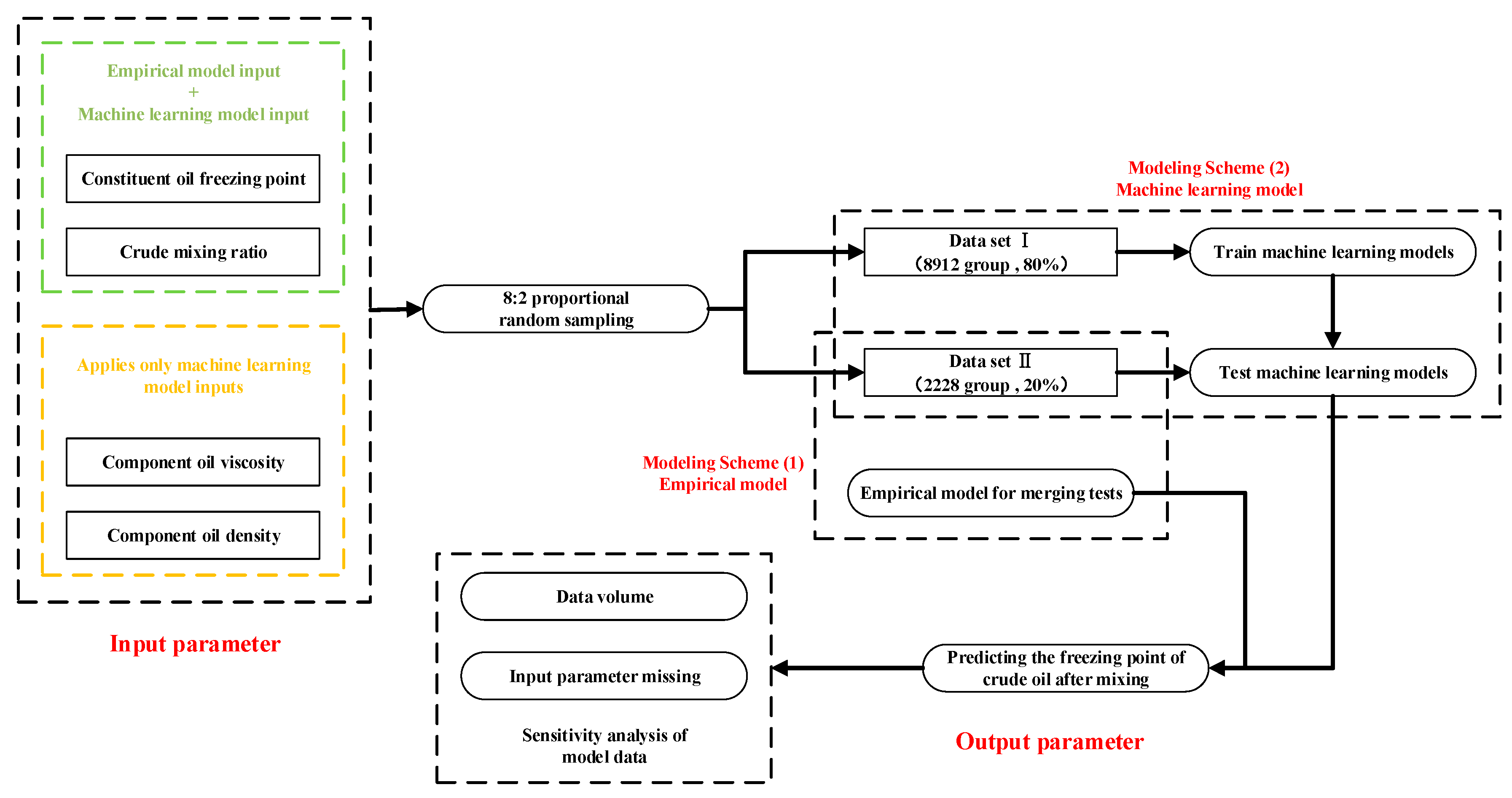
2.2. Model Procedure

Utilizing the ensemble machine learning framework, a tailored machine learning training process was devised. Illustrated in Figure 3, the process primarily encompasses three segments: data preprocessing, model design and training, and result evaluation.

2.2.1. Data Analysis

In both online and manual monitoring data for pipelines, human-recorded errors and data omissions or overlaps are common issues. When constructing the dataset, the first step involves developing data crawlers to integrate valid data scattered throughout daily monitoring reports. Subsequently, a stream-based data cleaning process is conducted, involving data alignment, outlier removal, and missing value imputation. By combining online monitoring data for comparison and supplementation, a clean dataset for predicting mixed crude oil properties is obtained. The dataset is then divided into training and testing sets and standardized to eliminate the influence of different input features’ dimensions and magnitudes, thereby reducing the risk of regression model overfitting. The min–max normalization formula is expressed as Equation (15):

$$x^{\prime }={\displaystyle \frac{\left(x-X_{\min }\right)}{\left(X_{\max }-X_{\min }\right)}}$$

(15)

where $x$ represents the original data, $x^{\prime }$ represents the standardized data, and X_max and X_min, respectively, denote the maximum and minimum values within a feature vector. The preprocessed training data is fed into the model for parameter iteration, and the trained model is tested using the testing set. Leveraging genetic algorithms, hyperparameters utilized for model training are continually optimized to reduce the cost of model retraining, enhance model performance, and improve its adaptability to newly introduced data.

2.2.2. Evaluation Criteria for Crude Oil Pour Point Prediction Models

To assess the predictive performance of regression models, two categories of metrics are introduced: ① classical metrics for evaluating machine learning models and ② evaluation metrics tailored for pour point prediction problems.

(1)

Classical machine learning evaluation metrics

The mean absolute deviation (MAD) is utilized to represent the average deviation level of model predictions, defined as shown in Equation (16). The Root Mean Square Deviation (RMSD) characterizes both the average deviation level and the dispersion of deviations in model predictions, defined as shown in Equation (17). The max absolute deviation (AD_max) denotes the maximum deviation level of model predictions, as shown in Equation (18). R² represents the coefficient of determination for regression, indicating the level of fit of the model to the target data. Its value ranges between 0 and 1, with a tendency towards 1 indicating a perfect model fit. Smaller values of Equations (16)–(19) indicate better model performance.

$$MAD={\displaystyle \frac{1}{n}}{\displaystyle \sum _{i=1}^n\left|{\widehat{y}}_i-y_i\right|}$$

(16)

$$RMSD=\sqrt{{\displaystyle \frac{1}{n}}{{\displaystyle \sum _{i=1}^n\left({\widehat{y}}_i-y_i\right)}}^2}$$

(17)

$$A{D}_{\max }=\max (\left|{\widehat{y}}_i-y_i\right|)$$

(18)

$$R^2=1-{\displaystyle \frac{{\displaystyle \sum _{i=1}^n}{\left({\widehat{y}}_i-y_i\right)}^2}{{\displaystyle \sum _{i=1}^n}{\left({\overline{y}}_i-y_i\right)}^2}}$$

(19)

where $y_i$ represents the measured values, ${\widehat{y}}_i$ represents the model predicted values, ${\overline{y}}_i$ represents the mean value of the sample measurements, and n is the number of samples.

(2)

Evaluation Metrics for Pour Point Prediction Models

The standard SY/T0541-2009 [18] “Test method for gel point of crude oils” of the People’s Republic of China’s petroleum and natural gas industry specifies: “Using the same operator, equipment, and laboratory facilities, following the procedures outlined in the method, repeated measurements of the same oil sample should be performed over a continuous period. The difference between the results of two consecutive measurements should not exceed 2 °C”. This standard leads to the derivation of the pour point absolute deviation (deviation percentage), denoted as Dp. Dp represents the proportion of data points with absolute deviations outside the given interval [0, 2]. Dp is defined as shown in Equation (20).

$$D_{\mathrm{p}}={\displaystyle \frac{n\left\{\left|y_i-{\widehat{y}}_i\right|>2\right\}}{N}}\times 100\%$$

(20)

where $n\left\{\left|y_i-{\widehat{y}}_i\right|>2\right\}$ represents the samples with prediction deviations exceeding 2 °C and $N$ represents the total number of samples.

The error result is that the difference between the predicted value and the experimental is more than 2 °C. The smaller the values of MAD, RMSD, AD_max, and D_p, the more accurate the model prediction results. And the closer the R² value is to 1, the better the fitting degree of the regression model.

3. Numerical Analysis

3.1. Data Infrastructure

Experimental verification and comparative analysis were performed using a scenario involving the blending and exportation of crude oil with four components. The process of blending the four types of crude oil and their subsequent exportation is depicted in Figure 4.

The dataset of crude oil properties originates from on-site manual sampling tests conducted over a span of 10 years in pipelines, yielding a total of 11,140 sample sets. These property data encompass the pour point, density, viscosity at 20 s⁻¹, and blend ratio of mixed crude oil under various compositions of the four components. Density at 20 °C and viscosity at 15 °C are required as per on-site production standards, with temperature adjustments precisely regulated during manual testing. In cases where online measurement data are employed, oil temperatures tend to fluctuate. For density data, a well-established petroleum density conversion method (Equation (21)) can be utilized to convert to a density ${\rho }_{20}$ at 20 °C. In the equation, $\gamma$ denotes the temperature coefficient of petroleum density, which can be obtained from a reference table.

$${\rho }_{20}={\rho }_t+\gamma \left(t-20\right)$$

(21)

For viscosity, the viscosity data obtained from online instruments can be converted to viscosity at 15 °C based on the corresponding viscosity–temperature relationship for crude oil.

The statistical summary of the physical properties for the component crude oils is provided in

Table 2. Statistical results of oil property monitoring data.

Crude Oil ID	Range (°C)	Mean (°C)	Standard Deviation (°C)	15 °C, 20 s−1 Viscosity (mPa·s)	Density of 20 °C (kg/m3)
Crude Oil 1	−24~0	−10.47	5.00	20~80	855~875
Crude Oil 2	−23~10	−0.62	5.30	10~250	830~890
Crude Oil 3	−28~5	−12.83	8.44	5~450	800~860
Crude Oil 4	−16~22	−11.98	4.17	5~500	810~870

, illustrating the complexity, significant variations, and considerable fluctuations in properties among the transported crude oils.

3.2. Modeling Strategy

Figure 5 presents the modeling scheme for predicting the pour point of blended crude oil using both empirical and machine learning models. To quantitatively assess the accuracy and applicability of these models, we employed the holdout method to partition the total dataset into two subsets: Dataset I, which accounts for 80% of the total data (8912 sets), and Dataset II, which comprises 20% of the total data (2228 sets). The testing schemes based on these datasets are outlined as follows:

(1) For the empirical model (Equations (1), (4)–(6)), Dataset II (2228 sets) was utilized for fitting and testing. The pour points of individual component crude oils before blending, along with their blend ratios, served as inputs, while the pour point of the blended crude oil was the output.

(2) Regarding machine learning models based on different principles, Dataset I (8912 sets) was employed for model training, while Dataset II (2228 sets) was used for model validation. The pour points, viscosity, density, and blend ratios of individual component crude oils before blending were considered as potential inputs, with the pour point of the blended crude oil as the output. Additionally, we examined the stability of the machine learning models under various multi-dimensional data feature patterns, such as changes in data volume and missing input data.

3.3. Prediction Results

3.3.1. Validation Results of the Empirical Model

Testing was conducted based on modeling approach (1). In the scenario where pour point data for blended crude oil with two component oils at equal ratios were unavailable, the prediction results of each empirical model are outlined in

Table 3. Comparison of prediction performance of different empirical models.

Model	MAD (°C)	RMSD (°C)	R2	Dp (%)	ADmax (°C)
Equation (1)	3.77	5.25	0.76	7.7	15.07
Equation (4)	2.65	4.74	0.89	9.6	13.06
Equation (5)	2.87	4.39	0.86	8.5	11.07
Equation (6)	3.17	4.62	0.82	8.2	12.19

.

As observed, Equation (4) demonstrates higher predictive accuracy, with an average absolute deviation of 2.65 °C, whereas Equation (6) exhibits better stability, with a proportion of prediction deviations exceeding 2 °C at 8.2%.

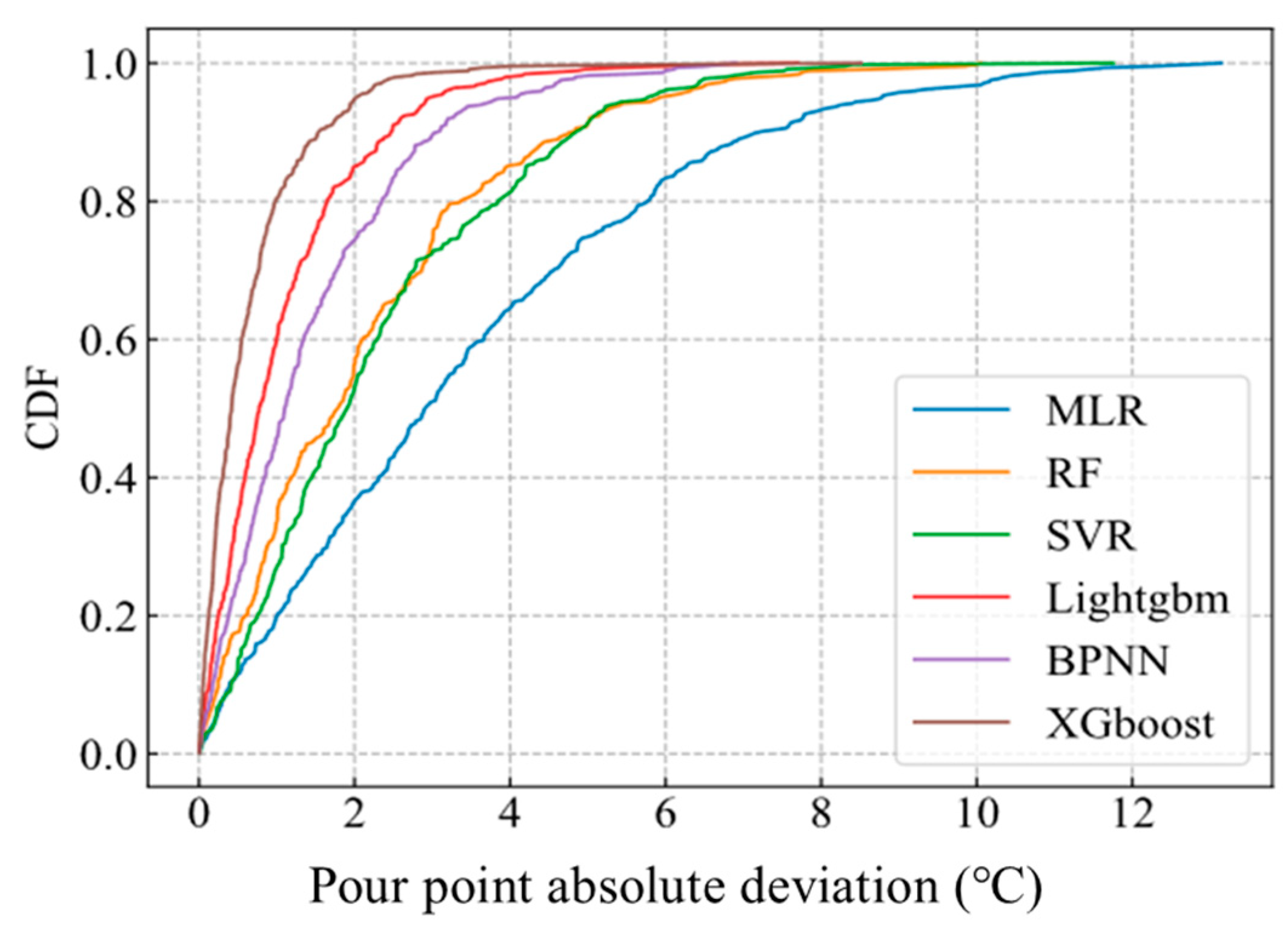
3.3.2. Experimental Results of Machine Learning Models

We conducted experiments on six different machine learning models based on multiple linear regression (MLR), support vector machine (SVR), random forest (RF), backpropagation neural network (BPNN), LightGBM, and XGBoost, as described in references [19,20,21]. The training hyperparameters of the models were randomly initialized and optimized using a genetic algorithm to ensure that the final trained models possessed the best capabilities under their respective principles. Figure 6 illustrates the prediction results of the six machine learning models. Detailed statistical metrics are provided in

Table 4. Comparison of performance of different machine learning models.

Model	MAD (°C)	RMSD (°C)	R2	Dp (%)	ADmax (°C)
MLR	4.03	5.25	0.69	19.56	15.31
RF	2.83	3.74	0.74	17.96	13.71
BPNN	1.70	2.06	0.92	12.80	7.68
SVR	2.17	5.39	0.85	13.26	12.10
LightGBM	2.21	2.86	0.89	15.81	10.04
XGBoost	1.12	1.74	0.94	11.98	5.28

. If accuracy is considered the primary criterion, XGBoost performs the best. It is mainly due to the deep extraction of input features and the accurate loss function using second-order Taylor expansion and the superior generalization performance of ensemble learning and over fitting of the tree avoided by adding regularization. While the MLR model has the simplest structure, it exhibits larger prediction errors and a higher probability of extreme prediction values. The main reason is that the MLR model is relatively simple, cannot capture and learn the nonlinear relationship, and will be unstable in the case of feature redundancy (i.e., multicollinearity) [22,23]. In comparison, SVR, BPNN, and LightGBM demonstrate slightly stronger learning capabilities with moderate prediction performance. Among the six machine learning prediction models, XGBoost shows a more concentrated distribution of prediction results and superior prediction stability.

Figure 7 gives the cumulative probability distribution (CDF) of absolute error of the predicted model. It describes the instability of model prediction results due to fluctuations of physical property parameters and measurement errors. The developed XGBoost model presents a good ability of prediction deviation, and the prediction performance is more reliable than other models [24].

Based on the comprehensive analysis of Table 3 and Table 4, in conjunction with Figure 6 and Figure 7, it is evident that the predictive accuracy of the XGBoost ensemble machine learning model is significantly enhanced compared to the empirical model.

3.3.3. Model Sensitivity Analysis

(1)

Sensitivity of Models to Data Volume

The predictive performance of a developed machine learning model is directly related to the amount of data used for training. In other words, considering the number of dataset samples, sensitivity analysis experiments are carried out on the empirical equation and the XGBoost model with the best performance above. Samples are generated by random sampling of total samples, the sampling proportion varies from 0.01 to 1, the step size is 0.01, that is, the minimum sample number is 112 groups, and the maximum sample number is 11,140 groups. The indicator MAE is calculated when the samples are generated. The variation of MAE with the increasing sample size is shown in Figure 8.

The empirical model is closely related to the data. When the data quality is high, the empirical model with higher precision can be fitted with less data. When the data quality is not high, the small amount of data makes it difficult to effectively determine the fitting parameters. The prediction of the pour point of mixed crude oil may fall into this category. With a small amount of data, the accuracy of the empirical equation is higher than that of the machine learning model, but with the accumulation of the number of samples, the performance of the machine learning model is significantly better than the empirical equation [25]. The main reasons for the poor accuracy of the empirical equation are as follows: the selected empirical model is related to the data, and the accuracy of the pour point data with 1:1 equal ratio of non-component oil is lower than that of the empirical equation with physical property information with an equal ratio of component oil. The data time span is large, resulting in a large difference in physical properties. The empirical model is applicable to oil products within a certain time range and oil products with no great change in physical properties.

Figure 8a demonstrates that, within the scope of this study, the predictive accuracy of empirical models is virtually unaffected by the number of samples. In contrast, machine learning models exhibit a clear dependence on sample size. With limited data volume, the accuracy of empirical models surpasses that of machine learning models. However, as the sample size increases, the performance of machine learning models becomes notably superior to that of empirical models [26]. The predictive power of the machine learning model decreases significantly with the reduction of the amount of training data, mainly because with too little training data, it is difficult for the machine learning model to learn features and inter-relationships at multiple levels, which correspondingly increases the difficulty of model training and prediction. In the case of sufficient data, the predictive power of the model will decrease with the increase in the fluctuation amplitude of components in the data, but the predictive performance will not change significantly in this case. This is mainly because the machine learning model ensures that it has a certain generalization ability to effectively deal with the interference introduced by the difference in the data.

In the early stages of engineering applications, where data volume is scarce, empirical models may be initially employed. As the data volume accumulates to a certain extent (e.g., 1000 samples), machine learning models with self-improvement mechanisms can be utilized to ensure that the average absolute deviation of pour point prediction for blended crude oils is controlled within 2 °C, as shown in Figure 8b.

(2)

Sensitivity Analysis of Models to Missing Input Parameters

In the production of oil pipelines, it is common to encounter scenarios where certain parameters are missing. Fundamentally, the definition of crude oil involves parameters such as density, viscosity, and pour point, which serve as inputs or outputs in the oil transportation process. Missing data for these parameters can lead to a misalignment in the model’s characterization of crude oils, thereby impacting predictive accuracy. For empirical models, the absence of pour points for component crude oils renders the prediction of pour points for blended crude oils impossible. Machine learning possesses the advantage of robustly extracting deep information from data. In this study, the robustness of the XGBoost model was validated under four scenarios of missing data. The specifics of the five testing scenarios are detailed in

Table 5. Scenarios for missing data.

Scenarios	Data Gaps	The Minimum Sample Size Required for an Average Absolute Deviation below 2 °C
1	The density (ρ) of the crude oil at 20 °C and the viscosity (μ) of the crude oil at 15 °C	4213
2	the viscosity (μ) of the crude oil at 15 °C	4122
3	The density (ρ) of the crude oil at 20 °C	3454
4	The pour point (Tg) of the crude oil components	6796
5	No Missing Values	892

.

The predictive outcomes of the model under different scenarios of data absence are depicted in Figure 9.

As expected, the predictive accuracy decreases to varying degrees when input data is missing, such as the viscosity of crude oil components (Scenario 2), the density of crude oil components (Scenario 3), or both (Scenario 1), compared to the scenario with no missing input data (Scenario 5). Moreover, when the input parameters include only the density and viscosity of crude oil components (Scenario 4, i.e., missing the pour point of crude oil components), the predictive accuracy decreases the most. However, it is noteworthy that with a large data volume (6796 sets), the model’s predictions maintain an average absolute deviation within 2 °C (1.96 °C, 1.98 °C, 1.83 °C, 2.00 °C, and 1.48 °C for Scenarios 1 to 5, respectively), indicating practical applicability in engineering. This underscores the significance of leveraging machine learning methods to address the challenge of online pour point prediction, especially considering the maturity of online measurement technologies for viscosity and density compared to pour point measurement. In addition, when the accuracy of the model reaches the bottleneck value, an additional order of magnitude increase in the amount of data is needed to further improve the accuracy of the model. However, with the increase in the amount of data, the improvement effect of the introduced input parameters on the model is gradually weakened [25].

It is important to acknowledge that machine learning models rely on the training dataset. Thus, the accuracy of the model should be verified when new crude oil varieties are introduced or when the model is transferred to different pipelines, representing crude oils with diverse compositions and properties. Nevertheless, the methodology investigated in this study holds potential for broader application.

4. Conclusions

This study addresses the prediction of pour points for blended crude oils from different sources, based on the physical property data of a specific pipeline crude oil. A comprehensive comparison was conducted among six different types of machine learning models: multiple linear regression, random forest, support vector machine, LightGBM, backpropagation neural network, and XGBoost. Additionally, the XGBoost ensemble machine learning model, which exhibited optimal performance, was compared with empirical models. Furthermore, the sensitivity of machine learning models and empirical models was analyzed in terms of data volume and missing input parameters. Key findings are as follows:

(1) Empirical models exhibit less sensitivity to the amount of fitting data, while machine learning models are more sensitive. Therefore, in situations with limited data, empirical models can be used for prediction. As the amount of data increases, a combination of empirical and machine learning models can be employed, transitioning ultimately to machine learning models.

(2) The XGBoost ensemble machine learning model demonstrated the highest predictive performance. With inputs including blend ratio, pour points, viscosity, and density of component crude oils, under the condition of 8912 training datasets, the average absolute deviation of predictions was 1.12 °C, with 88% of predictions having deviations within 2 °C. This predictive accuracy far exceeds that of empirical models (with average absolute deviations all exceeding 2 °C).

(3) The predictive accuracy of the XGBoost model decreases when the physical properties of component crude oils are missing to varying degrees. However, under the aforementioned training data condition, the average absolute deviation of pour points remains within 2 °C. Notably, when pour points of component crude oils are missing, the average absolute deviation of pour points for blended crude oils is 1.93 °C, when using blend ratio, viscosity, and density of component crude oils as inputs. This indicates that leveraging the powerful data mining capabilities of machine learning models can address the issue of online prediction of pour points for blended crude oils in the presence of missing data (such as pour points of component crude oils) encountered in production.

References

1. Xu, H.; Wang, Y.; Wang, K. Review on the gelation of wax and pour point depressant in crude oil multiphase system. Int. J. Mod. Phys. B 2021, 35, 2130005. [Google Scholar] [CrossRef]
2. Jinjun, Z.; Bo, Y.; Hongying, L.; Qiyu, H. Advances in rheology and flow assurance studies of waxy crude. Pet. Sci. 2013, 10, 538–547. [Google Scholar]
3. Srikanth, B.; Papineni, S.-L.; Sridevi, G.; Indira, D.-N.-V.-S.; Radhika, K.-S.-R.; Syed, K. Adaptive XGBOOST Hyper Tuned Meta Classifier for Prediction of Churn Customers. Intell. Autom. Soft Comput. 2022, 33, 21–34. [Google Scholar] [CrossRef]
4. Li, Y.; Zhang, J. Prediction of Viscosity Variation for Waxy Crude Oils Beneficiated by Pour Point Depressants During Pipelining. Pet. Sci. Technol. 2005, 23, 915–930. [Google Scholar] [CrossRef]
5. Liu, T.; Sun, W.; Gao, Y.; Xu, C. Study on the Ordinary Temperature Transportation Process of Multi-blended Crude oil. Oil Gas Storage Transp. 1999, 18, 1–7. [Google Scholar]
6. Li, N.; Mao, G.; Shi, X.; Tian, S.; Liu, Y. Advances in the research of polymeric pour point depressant for waxy crude oil. J. Dispers. Sci. Technol. 2018, 39, 1165–1171. [Google Scholar] [CrossRef]
7. Chen, J.; Zhang, J.; Zhang, F. A new model for determining gel points of mixed crude. J. Univ. Pet. China 2003, 27, 76–80. [Google Scholar]
8. Loskutova, Y.-V.; Yudina, N.-V. Prediction of the effectiveness of pour-point depressant additives from data on the antioxidant properties of crude oil. Chem. Technol. Fuels Oils 2015, 50, 483–488. [Google Scholar] [CrossRef]
9. Majhi, A.; Sharma, Y.-K.; Kukreti, V.-S.; Bhatt, K.-P.; Khanna, R. Wax Content of Crude Oil: A Function of Kinematic Viscosity and Pour Point. Pet. Sci. Technol. 2015, 33, 381–387. [Google Scholar] [CrossRef]
10. Hou, L.; Xu, X.; Liu, X. Application of BP Neural Network in the Gel Point Prediction of Blend Crude Oil. J. Petrochem. Univ. 2009, 3, 86–88. [Google Scholar]
11. Hu, K.; Zhang, F.; Wang, S.; Zhang, Y.; Zhang, Y.; Liu, K.; Gao, Q.; Meng, X.; Meng, J. Application of bayesian regularized artificial neural networks to predict pour point of crude oil treated by pour point depressant. Pet. Sci. Technol. 2017, 35, 1349–1354. [Google Scholar] [CrossRef]
12. Khamehchi, E.; Mahdiani, M.-R.; Amooie, M.-A.; Hemmati-Sarapardeh, A. Modeling viscosity of light and intermediate dead oil systems using advanced computational frameworks and artificial neural networks. J. Pet. Sci. Eng. 2020, 193, 107388. [Google Scholar] [CrossRef]
13. Li, B.; Guo, Z.; Zheng, L.; Shi, E.; Qi, B. A comprehensive review of wax deposition in crude oil systems: Mechanisms, influencing factors, prediction and inhibition techniques. Fuel 2024, 357, 129676. [Google Scholar] [CrossRef]
14. Arabameri, A.; Pal, S.-C.; Costache, R.; Saha, A.; Rezaie, F.; Danesh, A.-S.; Pradhan, B.; Lee, S.; Hoang, N.-D. Prediction of gully erosion susceptibility mapping using novel ensemble machine learning algorithms. Geomat. Nat. Hazards Risk 2021, 12, 469–498. [Google Scholar] [CrossRef]
15. Zhou, Y.; Li, T.; Shi, J.; Qian, Z.; Marisol, B.-C.; Correia, M.-B. A CEEMDAN and XGBOOST-Based Approach to Forecast Crude Oil Prices. Complexity 2019, 2019, 4392785. [Google Scholar] [CrossRef]
16. Nguyen, H.; Cao, M.-T.; Tran, X.-L.; Tran, T.-H.; Hoang, N.-D. A novel whale optimization algorithm optimized XGBoost regression for estimating bearing capacity of concrete piles. Neural Comput. Appl. 2023, 35, 3825–3852. [Google Scholar] [CrossRef]
17. Sheng, K.; He, Y.; Du, M.; Jiang, G. The Application Potential of Artificial Intelligence and Numerical Simulation in the Research and Formulation Design of Drilling Fluid Gel Performance. Gels 2024, 10, 403. [Google Scholar] [CrossRef] [PubMed]
18. SY/T0541-2009; Test Method for Gel Point of Crude Oils. National Energy Administration: Beijing, China, 2009.
19. Saleh, A.; Yuzir, A.; Sabtu, N.; Abujayyab, S.K.; Bunmi, M.-R.; Pham, Q.-B. Flash flood susceptibility mapping in urban area using genetic algorithm and ensemble method. Geocarto Int. 2022, 37, 10199–10228. [Google Scholar] [CrossRef]
20. Gu, Z.; Cao, M.; Wang, C.; Yu, N.; Qing, H. Research on Mining Maximum Subsidence Prediction Based on Genetic Algorithm Combined with XGBoost Model. Sustainability 2022, 14, 10421. [Google Scholar] [CrossRef]
21. Wang, M.; Xie, Y.; Gao, Y.; Huang, X.; Chen, W. Machine learning prediction of higher heating value of biochar based on biomass characteristics and pyrolysis conditions. Bioresour. Technol. 2024, 395, 130364. [Google Scholar] [CrossRef]
22. Hanna, E.G.; Younes, K.; Amine, S.; Roufayel, R. Exploring Gel-Point Identification in Epoxy Resin Using Rheology and Unsupervised Learning. Gels 2023, 9, 828. [Google Scholar] [CrossRef]
23. Mo, T.; Li, S.; Li, G. An interpretable machine learning model for predicting cavity water depth and cavity length based on XGBoost–SHAP. J. Hydroinform. 2023, 25, 1488–1500. [Google Scholar] [CrossRef]
24. Dhankar, S.; Sharma, D.; Mohanta, H.-K.; Sande, P.-C. Machine Learning Applied to Predict Key Petroleum Crude Oil Constituents. Chem. Eng. Technol. 2024, 47, 365–374. [Google Scholar] [CrossRef]
25. Ganesh, S.; Ramakrishnan, S.K.; Palani, V.; Sundaram, M.; Sankaranarayanan, N.; Ganesan, S.-P. Investigation on the mechanical properties of ramie/kenaf fibers under various parameters using GRA and TOPSIS methods. Polym. Compos. 2022, 43, 130–143. [Google Scholar] [CrossRef]
26. Lennon, K.-R.; Rathinaraj, J.-D.-J.; Cadena, M.-A.G.; Santra, A.; McKinley, G.-H.; Swan, J.-W. Anticipating gelation and vitrification with medium amplitude parallel superposition (MAPS) rheology and artificial neural networks. Rheol. Acta 2023, 62, 535–556. [Google Scholar] [CrossRef]
Figure 1. Pour point prediction models of mixed crude oil and their relationship.
Processes 12 01783 g001
Figure 2. Training flow chart of XGBoost model.
Processes 12 01783 g002
Figure 3. Flow charts of machine learning construction.
Processes 12 01783 g003
Figure 4. Pipeline structure of four-source-mixed oil transportation.
Processes 12 01783 g004
Figure 5. Modeling scheme of pour point prediction based on empirical model and machine learning model.
Processes 12 01783 g005
Figure 6. Box plot of pour point prediction error based on machine learning.
Processes 12 01783 g006
Figure 7. CDF performance comparison based on absolute deviation of condensation point prediction results.
Processes 12 01783 g007
Figure 8. Data sensitivity analysis of pour point prediction model; (a) data sensitivity based on empirical models; (b) data sensitivity based on machine learning models.
Processes 12 01783 g008
Figure 9. Mean absolute error with different data missing scenarios.
Processes 12 01783 g009