Adaptive Finite-Time Constrained Attitude Stabilization for an Unmanned Helicopter System under Input Delay and Saturation

Abstract

This study focuses on addressing the constrained attitude stabilization problem for an unmanned helicopter (UH) system subject to disturbances, input delay and actuator saturation. A constrained memory sliding mode is first presented to constrain the flight attitude while handling the input delay. On this basis, an adaptive finite-time nonlinear observer is proposed to estimate the lumped disturbance with unknown upper bound. Moreover, based on the hyperbolic tangent function, a saturated attitude controller is designed to tackle the input saturation problem via the adaptive laws. The finite-time stability of the closed-loop constrained attitude system is proved by Lyapunov synthesis. Finally, the developed scheme can accomplish attitude stabilization and overcome the influence of disturbances, attitude constraint, input delay and actuator saturation in an easy way. Numerical simulations are carried out to demonstrate the effectiveness of the proposed control scheme.

1. Introduction

Attitude stabilization control has received considerable attention due to its important role in UH systems. However, complex nonlinear characteristics such as actuator saturation, input delay, state constraints, parametric uncertainty and external disturbances greatly increase the difficulty and complexity of controller design. In recent years, to overcome these problems, many improvements have been extensively investigated in the literature via several inspiring approaches, to name a few, backstepping control, H∞, sliding mode control (SMC), adaptive control and intelligent optimal control [1,2,3,4,5,6,7].

Compared with a manned helicopter, a UH typically has smaller fuselage and lighter mass, which makes it more sensitive to external disturbances. Meanwhile, with the expansion of flight envelope, the uncertainties caused by the estimations of a UH’s centroid and aerodynamic parameters will further weaken the attitude control stability. Using a disturbance observer and introducing SMC robustness terms are two effective methods to deal with external disturbances and system uncertainties [8,9,10]. In [11], many disturbance-observer-based control schemes have been summarized and reviewed, where the fuzzy mechanism (FM), the neural network (NN) and nonlinear disturbance observer (NDO) were widely studied and applied in UH attitude systems [12,13,14]. Although the FM and the NN have the universal approximation ability for the unknown nonlinear functions, the fuzzy and the NN training algorithms demand huge computation power. Compared with those two methods, the NDO with robustness term is more practical due to having fewer design parameters and training costs [15,16,17]. In [15], an NDO was utilized to handle the influence of external disturbances. To reduce the inherent chattering of SMC and improve the system robustness, an improved NDO was proposed for the spacecraft platform in [16]. Nowadays, modern flight tasks require UHs to achieve control objectives within a finite time for rapid-response and anti-disturbance abilities. A second-order NDO was developed in [17] to reconstruct the lumped disturbances in finite time. It is noted that the methods in [15,16] cannot achieve finite-time convergence, while the method in [17] requires the differential upper bounds of disturbance. Therefore, how to design a feasible NDO that can achieve finite-time convergence without knowing the disturbance upper bound is of great significance.

Constraints seriously restrict attitude stability performance, especially output constraint and actuator saturation, which are inevitably encountered during flight [18,19,20]. To prevent the violation of state constraints, the barrier Lyapunov function (BLF) is a very effective tool. Combining the backstepping method and BLF, two adaptive constrained control schemes were developed for the systems with state and output constraints in [21,22]. Taking the actuator saturation into account, several anti-saturation strategies have been studied [23,24], in which the Nussbaum function or saturation compensator are widely applied. The FM or NN were also utilized to integrate the BLFs to improve control performance and deal with the input or output constraints [25,26]. It is worth noting that most of the above methods are passively compensation input saturation and are unable to achieve finite-time convergence. In addition, the influence of input delay is ignored in the controller design.

In actual attitude control, due to the aging of sensors and actuators, the speeds of receiving and processing external signals are different. As a result, the input delay and communication delay will be generated [27,28], which seriously threaten the control stability. In [29], a backstepping-based adaptive controller was proposed for a class of uncertain systems with unknown constant-time input delay. In [30], an NDO-based auxiliary system is applied to compensate the effect of the input delay for a quadrotor unmanned aerial vehicle with disturbances. By employing the Pade approximation, an intermediate variable method is developed to eliminate the effect of the input delay in [31]. Using the Razumikhim method, a memoryless controller has been designed in [32], while in [33,34], memory controllers have been developed via the Lyapunov–Krasovskii functional approach. Unfortunately, these methods need to know precise delay time in advance, and the Pade approximation method may be not effective for large-scale delays, so further improvements can be made. In addition, to the best of the authors’ knowledge, there are few control methods that have solved the input delay problem while simultaneously overcoming the problems of actuator saturation, output constraints and unknown perturbations for the UH attitude system.

Inspired by the above discussion and analysis, a novel adaptive finite-time constrained attitude controller is investigated for the UH attitude system subject to disturbance, input delay and actuator saturation. In summary, the innovations are listed below.

(1)

In this paper, the problem of attitude stabilization control with output constraints, actuator saturation, input delay and external disturbance is considered. The dependence on precise input delay and the upper bound of disturbance is relaxed; thus, the control scheme is more concise.

(2)

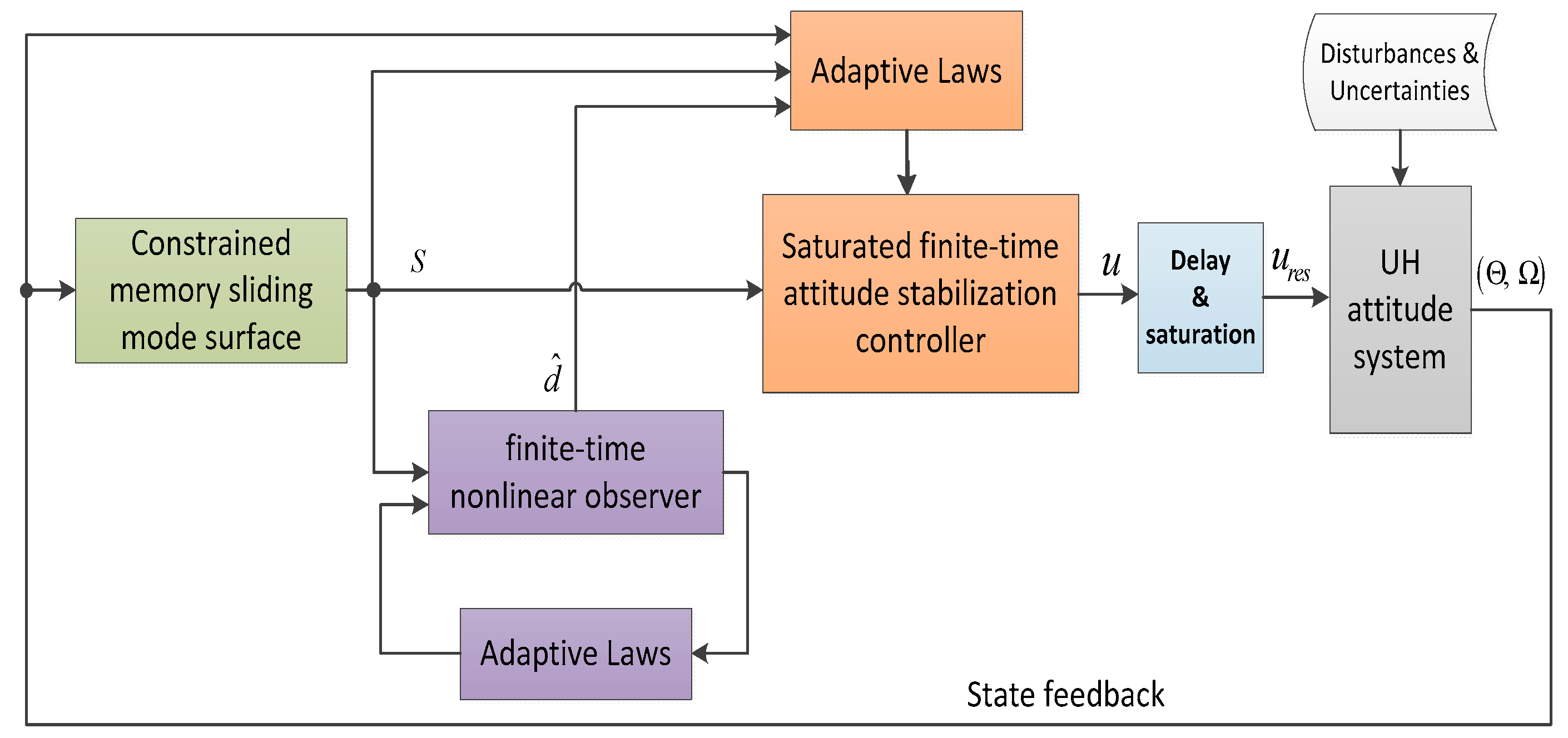
By integrating the BLF and input memory compensation, a novel constrained memory sliding mode (CMSM) is designed to handle the input delay and attitude constraints. On this basis, an adaptive finite-time nonlinear observer (AFNO) is designed for quickly estimating the external interference and unknown delay deviation.

(3)

Based on CMSM and AFNO, a saturated finite-time attitude stabilization controller (SFASC) is designed to tackle the input saturation problem via the adaptive laws. By using Lyapunov analysis, the constrained attitude can converge to zero in finite time despite the disturbance, input delay and actuator saturation.

The remainder of this article is organized as follows. The problem formulation and some preliminaries are addressed in Section 2. The adaptive finite-time constrained attitude stabilization control scheme is presented in Section 3. In Section 4, simulation studies are given to validate the proposed control method. The final conclusions are given in Section 5.

2. Problem Formulation and Preliminaries

2.1. Attitude Dynamics

The attitude system of an UH is considered with input delay, actuator saturation, attitude constraints and unknown disturbances. The attitude dynamics are given as follows [3,13].

$$\left\{\begin{array}{c}\dot{\Theta }(t)=\mathrm{H}(\Theta )\Omega \hfill \\ \dot{\Omega }=-I_m^{-1}{S}_k\left(\Omega \right)I_m\Omega +I_m^{-1}{\Gamma }_u+d_{\tau }\hfill \end{array}\right.$$

(1)

where $\Theta ={[\begin{array}{ccc}\varphi & \theta & \psi \end{array}]}^T$ denotes the attitude angles, $\Omega ={[\begin{array}{ccc}p& q& r\end{array}]}^T$ denotes the angular rates, $I_m=diag(I_{xx},I_{yy},I_{zz})$ denotes the inertia matrix, ${\Gamma }_u$ denotes the total control torque and $d_{\tau }(t)$ denotes the unmodeled uncertainty and unknown external disturbance. The attitude kinematic matrix $\mathrm{H}(\Theta )$ and skew symmetric matrix $S_k\left(\Omega \right)$ are represented as

$$\begin{array}{l}\mathrm{H}(\Theta )=\left[\begin{array}{ccc}1& s_{\varphi }{s}_{\theta }/c_{\theta }& c_{\varphi }{s}_{\theta }/c_{\theta }\\ 0& c_{\varphi }& -s_{\varphi }\\ 0& s_{\varphi }/c_{\theta }& c_{\varphi }/c_{\theta }\end{array}\right]\\ S_k\left(\Omega \right)=\left[\begin{array}{ccc}0& -r& q\\ r& 0& -p\\ -q& p& 0\end{array}\right]\end{array}$$

where $s_{(•)}$ and $c_{(•)}$ represent the functions $\sin (•)$ and $\cos (•)$, respectively.

${\Gamma }_u$ can be expressed as

$${\Gamma }_u=I_m\left(A\Omega +Bu\right)$$

(2)

where $A$ and $B$ are constant matrices of appropriate dimensions with $rank(B)=3.$ $u=\left[{\delta }_{lon},{\delta }_{lat},{\delta }_{ped}\right]$ are the control inputs to be designed, where ${\delta }_{lon}$, ${\delta }_{lat}$ and ${\delta }_{ped}$ are the lateral cyclic control input, longitudinal control cyclic input and tail rotor control input, respectively. The model parameters $I_m$, $A$ and $B$ can be obtained through parameter identification and flight tests [3].

Due to physical limitations on actuators, the inputs are limited by $‖u_i‖\le u_{Mi}$ and the saturated input $u_{res}$ can be represented as

$$u_{res}(i)=\left\{\begin{array}{cc}{u}_i\hfill & \left|u_i\right|\le u_{Mi}\hfill \\ u_{Mi}sign(u_i)\hfill & \left|u_i\right|>u_{Mi}, i=1,2,3\hfill \end{array}\right.$$

(3)

where $u_M$ is the saturated bound of $u$.

In addition, we consider that there exists an unknown input delay $\tau$ satisfying $\tau ={\tau }_0+\Delta \tau$, where ${\tau }_0$ is a known constant delay near $\tau$, and $\Delta \tau$ is the delay deviation with unknown bound $\overline{\Delta }:=\left\{\Delta \tau \in R:\left|\Delta \tau \right|\le \overline{\Delta }\right\}$.

Therefore, the attitude system (1) can be written as

$$\left\{\begin{array}{c}\dot{\Theta }=\mathrm{H}(\Theta )\Omega \hfill \\ \dot{\Omega }=-I_m^{-1}{S}_k(\Omega )I_m\Omega +A\Omega +B{u}_{res}(t-{\tau }_0)+d\hfill \end{array}\right.$$

(4)

where $d$ is the lump disturbance that can be described as

$$d=u_{res}(t-\tau )-u_{res}(t-{\tau }_0)+d_{\tau }$$

(5)

To further facilitate the control scheme design, the following assumptions are given.

Hypothesis 1 (H1).

All states of the system can be measured.

Hypothesis 2 (H2).

The lump disturbance is assumed to be bounded by an unknown positive constant as $‖d‖\le d_m$ for $i=1,2,3$.

The control objective has two parts.

• All the signals of the closed-loop control system are finite-time stable, and the states of system (1) converge to zero in finite time.
• The attitude angles are always within the prescribed constraint intervals, and the control input constraints are never violated despite the disturbances and input delay.

Remark 1.

Hypothesis 2 is reasonable. That is because $d_{\tau }$ primarily consists of the gravitation, wind interference and unknown tiny torques, which are usually bounded with $‖d_{\tau }‖\le d_1$. Since $‖u_{res}(t-\tau )-u_{res}(t-{\tau }_0)‖\le 2‖u_M‖\Delta \tau \le 2‖u_M‖\overline{\Delta }$ holds, observing Equation (5), $‖d‖\le 2u_M\overline{\Delta }+d_1=d_m$ makes sense.

2.2. Mathematical Preliminaries

The following definition and lemmas are listed, which are necessary for the controller design and stability analysis.

Definition 1

([35]). Consider the nonlinear system $\dot{x}=f(x)$ with the open region $C_{\mathsf{{\rm Y}}}$ containing the origin. A barrier Lyapunov function $V_b(x)$ is positive definite, continuous and differentiable in the region $C_{\mathsf{{\rm Y}}}$ satisfying $V_b(x)\le c_{BLF}$ for $\forall t\ge 0$ along the solution of $\dot{x}=f(x)$, where $c_{BLF}$ is a certain positive constant. As $x$ approaches the boundary of $C_{\mathsf{{\rm Y}}}$, one can have $V_b(x)\to \infty$. Generally, the BLF can be chosen as the following logarithmic function.

$$V_b={\displaystyle \frac{1}{2}}\log {\displaystyle \frac{k_b^2}{k_b^2-x^2}},$$

(6)

where $k_b\in R^{+}$ is the constraint on $x$. In the set $\left|x\right|<k_b$, it can be straightforward to verify that $V_b$ is a valid Lyapunov function candidate.

Lemma 1

([36]). For $x_i\in R$ and $0<\gamma \le 1$, the following inequality always holds:

$${\left({\displaystyle \sum _{i=1}^n\left|x_i\right|}\right)}^{\gamma }\le {\displaystyle \sum _{i=1}^n{\left|x_i\right|}^{\gamma }}$$

(7)

Lemma 2

([37,38]). For any $x\in R$ and $\zeta >0$, the following inequalities always hold:

$$0\le \left|x\right|-x\tanh ({\displaystyle \frac{x}{\varsigma }})\le \iota \varsigma$$

(8)

$$-x\tanh ({\displaystyle \frac{x}{\varsigma }})+\varsigma \tanh ({\displaystyle \frac{\left|x\right|}{\varsigma }})\le -\left|x\right|$$

(9)

where $\iota$ is the constant satisfying $\iota =e^{-(\iota +1)}$, i.e., $\iota =0.2785$.

Lemma 3

([39,40]). Consider the nonlinear system $\dot{x}=f(x)$. Choose a continuous Lyapunov function candidate $V_N(x)$. If its derivative satisfies

$${\dot{V}}_N(x)\le -\lambda V_N^{\gamma }(x)+{\eta }_N,$$

(10)

where $\lambda >0$, $0<\gamma <1$ and $0<{\eta }_N<\infty$, then the system state will be stable and bounded in finite time with the residual set

$$\underset{t\to T_{\gamma }}{\lim }{V}_N(x)\le {\left[{\displaystyle \frac{{\eta }_N}{\left(1-{\theta }_0\right)\lambda }}\right]}^{{\displaystyle \frac{1}{\gamma }}}$$

where $0<{\theta }_0<1$. The convergence time satisfies

$$T_{\gamma }\le t_0+{\displaystyle \frac{V_N^{1-\gamma }(t_0)}{{\theta }_0\lambda (1-\gamma )}}.$$

In particular, if ${\eta }_N=0$, then $\underset{t\to T_{\gamma }}{\lim }{V}_N(x)=0$, and the convergence time $T_{\gamma }$ is limited to the following range

$$T_{\gamma }\le t_0+{\displaystyle \frac{V_N^{1-\gamma }(t_0)}{\lambda (1-\gamma )}}.$$

3. Main Results and Analysis

This section focuses on three parts to implement the control scheme design, including a novel constrained memory sliding mode surface, a finite-time nonlinear observer with adaptive laws and a saturated finite-time attitude stabilization controller for the UH attitude system to achieve the proposed control objectives. The overall control strategy is shown in Figure 1.

3.1. Constrained Memory Sliding Mode Surface Design

For the purpose of the attitude stabilization under input delay and attitude constraints, a novel sliding mode surface is designed as

$$S=B^{-1}\left[\Omega +k_{\Theta }\chi (\Theta )\right]+{\displaystyle \underset{t-{\tau }_0}{\overset{t}{\int }}{u}_{res}(\alpha )d\alpha }$$

(11)

where $k_{\Theta }$ is a designed positive constant to ensure the stability of the sliding mode, ${\chi }_i(\Theta )=\log {\displaystyle \frac{{\delta }_i^2}{{\delta }_i^2-{\Theta }_i^2}},i=1,2,3$, and ${\delta }_i$ is the constrained boundary of ${\Theta }_i$. Notice that $B$ is of full rank, so its inverse exists. By substituting Equation (4) into Equation (11), the derivative of $S$ can be described as

$$\begin{array}{cc}\dot{S}\hfill & =B^{-1}\left[\dot{\Omega }+diag({\displaystyle \frac{k_{\Theta }{\Theta }_i}{{\delta }_i^2-{\Theta }_i^2}})\dot{\Theta }\right]+u_{res}(t)-u_{res}(t-{\tau }_0)\hfill \\ & =F+u_{res}(t)+\overline{d}\hfill \end{array}$$

(12)

where

$$\begin{array}{l}F=B^{-1}\left[-I_m^{-1}{S}_k(\Omega )I_m\Omega +A\Omega +diag({\displaystyle \frac{k_{\Theta }{\Theta }_i}{{\delta }_i^2-{\Theta }_i^2}})\mathrm{H}(\Theta )\Omega \right]\\ \overline{d}=B^{-1}d\end{array}$$

According to Hypothesis 2, one can obtain

$$\overline{d}(t)\le ‖B^{-1}‖‖d‖\le {\overline{d}}_m.$$

(13)

where ${\overline{d}}_m$ is the unknown bound of the new lump disturbance $\overline{d}$.

Obviously, when the states reach the sliding mode surface, $S=0$. If $u_{res}=0$ and $\Theta =0$ can be guaranteed, the angular velocity $\Omega$ will also converge to zero.

Remark 2.

Combining the BLF of $\Theta$ and the memory compensation of $u_{res}$, the proposed sliding mode surface has advantages over the methods in [17,38]. On one hand, it can be deduced that if $S$ is stable and bounded, the BLF must be bounded all the time. Thus, this indirectly restricts the attitude $\Theta$ within the boundary ${\Theta }_i<{\delta }_i,i=1,2,3$. On the other hand, the memory control input integral is introduced into $S$, so that the derivative of $S$ no longer contains $u_{res}(t-{\tau }_0)$. In this way, the control law can be designed directly for $u_{res}(t)$ via the conventional delay-free controller methods. Moreover, compared with the anti-delay method in [30], the proposed method does not need to know the accurate value of delay $\tau$. As for the Pade approximation method in [31], a large delay may make the approximation invalid, while the proposed method is still valid. Therefore, the proposed sliding surface has better practicability and expansibility.

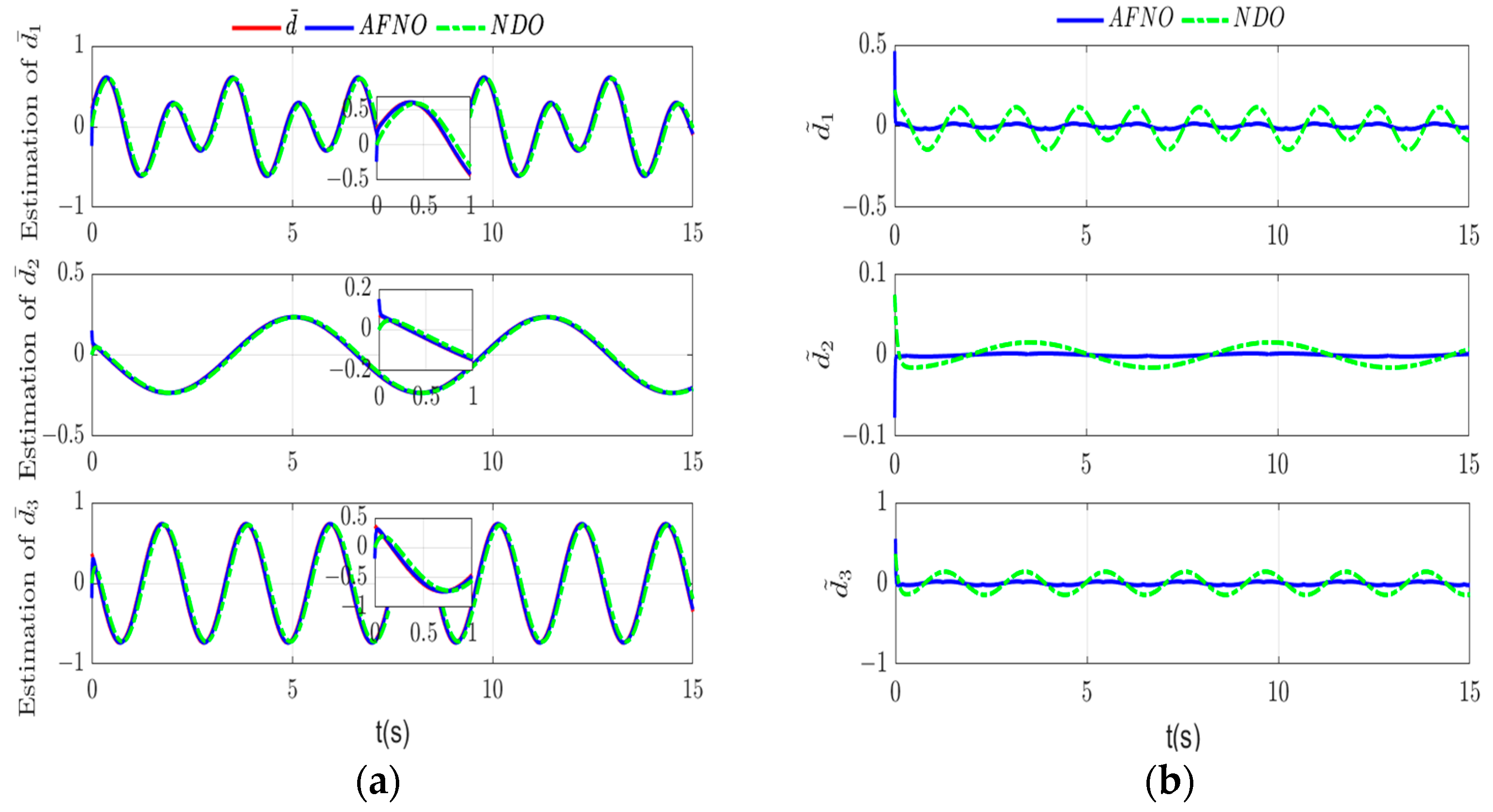
3.2. Adaptive Finite-Time Nonlinear Observer Design

To estimate the new lump disturbance $\overline{d}$, an adaptive finite-time nonlinear observer is designed as follow.

$$\left\{\begin{array}{c}\dot{\hat{S}}=F+u_{res}(t)+\hat{d}\hfill \\ \hat{d}=k_{o1}{e}_S+k_{o2}{e}_S^{\gamma }+\hat{\eta }\tanh ({\displaystyle \frac{e_S}{{\varsigma }_o}})\hfill \end{array}\right.$$

(14)

where $\hat{S}$ and $\hat{d}$ are the estimations of $S$ and $\overline{d}$, respectively. $e_S=S-\hat{S}$ is the estimation error of $S$, $k_{o1}$ and $k_{o2}$ are designed positive constants and ${\varsigma }_o$ is a small positive constant. $\hat{\eta }$ is a time-varying adaptive parameter of ${\overline{d}}_m$. $\gamma ={\alpha }_1/{\alpha }_2$, where ${\alpha }_1<{\alpha }_2$ are two positive odd integers.

Invoking Equation (12) and taking the derivative of $e_S$, one can yield

$${\dot{e}}_S=\dot{S}-\dot{\hat{S}}=\overline{d}-\hat{d}=\tilde{d}$$

(15)

where $\tilde{d}(t)$ is the estimation error of $\overline{d}$. It can be observed that guaranteeing $e_S$ to zero is equivalent to guaranteeing the disturbance estimation error $\tilde{d}(t)$ to zero.

The adaptive law for updating $\hat{\eta }$ is designed as

$$\left\{\begin{array}{c}\dot{\hat{\eta }}=-{\gamma }_o\left({\xi }_o\hat{\eta }+e_S^T\tanh ({\displaystyle \frac{e_S}{{\varsigma }_o}})\right)\\ {\gamma }_o={\displaystyle \frac{2a_0}{{\xi }_o(2a_0-1)}}{k_{o2}}^{{\displaystyle \frac{2}{\gamma +1}}}\end{array}\right.$$

(16)

where ${\xi }_o>0$ and $a_0>1/2$ are designed constants. Obviously, ${\gamma }_o>0$ holds.

Theorem 1.

Consider system (1), by applying the finite-time nonlinear observer (14) with the adaptive update laws (16), $\hat{S}$ can be governed to the neighborhoods of $S$ in finite time, and $\hat{d}$ converges to $\overline{d}$ in finite time.

Proof. 

Choose a Lyapunov function candidate as

$$V_O={\displaystyle \frac{1}{2}}{e}_S^T{e}_S+{\displaystyle \frac{1}{2{\gamma }_o}}{\tilde{\eta }}^2$$

(17)

where $\tilde{\eta }={\overline{d}}_m-\hat{\eta }$.

If ${\xi }_o>0$ and $a_0>1/2$, then one has ${\gamma }_o>0$. Combing Equations (14)–(16), the derivative of $V_O$ yields

$$\begin{array}{cc}{\dot{V}}_O=\hfill & e_S^T{\dot{e}}_S-{\gamma }_o^{-1}\tilde{\eta }\dot{\hat{\eta }}\hfill \\ & =-k_{o1}{e}_S^T{e}_S-k_{o2}{e}_S^T{e}_S^r+e_S^T\overline{d}(t)-\hat{\eta }{e}_S^T\tanh ({\displaystyle \frac{e_S}{{\varsigma }_o}})+{\xi }_o\tilde{\eta }\hat{\eta }-\tilde{\eta }{e}_S^T\tanh ({\displaystyle \frac{e_S}{{\varsigma }_o}})\hfill \\ & \le -k_{o1}{e}_S^T{e}_S-k_{o2}{e}_S^T{e}_S^r+{\overline{d}}_m\left[‖e_S^T‖-e_S^T\tanh ({\displaystyle \frac{e_S}{{\varsigma }_o}})\right]+{\xi }_o\tilde{\eta }\hat{\eta }\hfill \end{array}$$

(18)

Applying Lemma 2 and Young’s inequality, it follows

$$\begin{array}{cc}{\dot{V}}_O\le \hfill & -k_{o1}{e}_S^T{e}_S-k_{o2}{e}_S^T{e}_S^r-{\left[\left(1-{\displaystyle \frac{1}{2a_0}}\right){\xi }_o{\tilde{\eta }}^2\right]}^{{\displaystyle \frac{\gamma +1}{2}}}+{\left[\left(1-{\displaystyle \frac{1}{2a_0}}\right){\xi }_o{\tilde{\eta }}^2\right]}^{{\displaystyle \frac{\gamma +1}{2}}}\hfill \\ & -\left(1-{\displaystyle \frac{1}{2a_0}}\right){\xi }_o{\tilde{\eta }}^2+{\displaystyle \frac{2a_0}{2}}{\xi }_o{\eta }_m^2+3\iota {\varsigma }_o{\eta }_m\hfill \end{array}$$

(19)

Since $0<\gamma <1$ and ${\displaystyle \frac{1}{2}}<{\displaystyle \frac{\gamma +1}{2}}<1$, the following inequality holds.

$${\left[\left(1-{\displaystyle \frac{1}{2a_0}}\right){\xi }_o{\tilde{\eta }}^2\right]}^{{\displaystyle \frac{\gamma +1}{2}}}-\left(1-{\displaystyle \frac{1}{2a_0}}\right){\xi }_o{\tilde{\eta }}^2\le {\displaystyle \frac{1-\gamma }{1+\gamma }}{\left({\displaystyle \frac{2}{1+\gamma }}\right)}^{{\displaystyle \frac{-2}{1-\gamma }}}.$$

(20)

Using Lemma 1, one can obtain

$$\begin{array}{cc}{\dot{V}}_O\hfill & \le -2^{{\displaystyle \frac{\gamma +1}{2}}}{k}_{o2}{V_O}^{{\displaystyle \frac{\gamma +1}{2}}}+{\displaystyle \frac{1-\gamma }{1+\gamma }}{\left({\displaystyle \frac{2}{1+\gamma }}\right)}^{{\displaystyle \frac{-2}{1-\gamma }}}+{\displaystyle \frac{2a_0}{2}}{\xi }_o{\eta }_m^2+3\iota {\varsigma }_o{\eta }_m\hfill \\ & \le -{\lambda }_O{V_O}^{{\displaystyle \frac{\gamma +1}{2}}}+{\eta }_O\hfill \end{array},$$

(21)

where ${\lambda }_O=2^{{\displaystyle \frac{\gamma +1}{2}}}{k}_{o2}$ and ${\eta }_O={\displaystyle \frac{1-\gamma }{1+\gamma }}{\left({\displaystyle \frac{2}{1+\gamma }}\right)}^{{\displaystyle \frac{-2}{1-\gamma }}}+{\displaystyle \frac{a_0}{2}}{\xi }_o{\eta }_m^2+3\iota {\varsigma }_o{\eta }_m$.

According to Lemma 3, $V_O$ will converge to a small region in finite time $T_{\gamma }$.

$$T_{\gamma }\le {\displaystyle \frac{V_O^{1-\gamma }(0)}{{\theta }_0{\lambda }_O(1-\gamma )}},$$

The observer signals $e_S$ and $\tilde{\eta }$ are all stable and bounded with

$$e_S\le \sqrt{2{\left[{\displaystyle \frac{{\eta }_o}{\left(1-{\theta }_0\right){\lambda }_o}}\right]}^{{\displaystyle \frac{2}{\gamma +1}}}}$$

$$\tilde{\eta }\le \sqrt{2{\gamma }_o{\left[{\displaystyle \frac{{\eta }_o}{\left(1-{\theta }_0\right){\lambda }_o}}\right]}^{{\displaystyle \frac{2}{\gamma +1}}}}.$$

Thus, $\hat{S}$ will converge to a small neighborhood of $S$ in finite time. Considering Equations (14) and (15), $\hat{d}$ will converge to a small neighborhood of $\overline{d}$, accordingly. It can be seen that by increasing $k_{o2}$ and reducing ${\xi }_o$, the convergence neighborhood of the observation error will be sufficiently small. This completes the proof. □

Remark 3.

In Equation (12), since the differential of $S$ contains $\overline{d}$, we construct an estimation $\hat{S}$ for $S$ so that $\hat{d}$ can be introduced into $\hat{S}$ naturally, as shown in Equation (14). As long as the designed observer AFNO guarantees $\hat{S}\to S$ and $\dot{\hat{S}}\to \dot{S}$, one can obtain $e_S\to 0$ and ${\dot{e}}_S\to 0$. According to Equation (15), $\hat{d}$ will certainly converge to $\overline{d}$, which finally achieves the goal of lumped disturbance estimation.

Remark 4.

Compared with the classical NDO method in [30], the proposed method can achieve finite-time convergence. Compared with the observer based on the sliding mode method in [17], the proposed observer does not need to know the upper bound of the disturbances. Compared with the observer based on NN or FM methods in [12,13,14], the proposed observer is simpler and does not depend on extra parameter training. Therefore, this observer is more practical.

3.3. Saturated Finite-Time Attitude Stabilization Controller

It should be noticed that the control inputs are not allowed to violate the saturation constraints $u_M$. In this paper, unlike the compensation design and the Nussbaum-function-based methods in [17,23,24], a hyperbolic tangent function is used to directly design the saturated control law to overcome the input saturation problem. The adaptive saturated finite-time attitude stabilization controller is designed as follows.

$$u_{res}(t)=-U_m\tanh ({\displaystyle \frac{S}{{\kappa }_1{\xi }_c^2+{\kappa }_2{\vartheta }_c^2}})$$

(22)

where ${\kappa }_1$ and ${\kappa }_2$ are designed positive constants, and $U_m=diag(u_{mi}),i=1,2,3$ is the control gain. Meanwhile, $0<u_{mi}<u_{Mi}$ means that $‖u_{res}(t)‖<u_{Mi}$ will always hold; thus, the control inputs will never violate the saturation constraints. ${\xi }_c$ and ${\vartheta }_c$ are time-varying parameters with the adaptive laws as follows.

$$\left\{\begin{array}{c}{\dot{\varsigma }}_c=-{\sigma }_1\left[U_m{\kappa }_1{\varsigma }_c\tanh ({\displaystyle \frac{‖S‖}{{\kappa }_1{\xi }_c^2+{\kappa }_2{\vartheta }_c^2}})-{\gamma }_{c1}\tanh ({\displaystyle \frac{{\xi }_c}{\varsigma }})-{\displaystyle \frac{\mu M{\xi }_c^{-1}}{{\vartheta }_c^2+\mu }}\right]\hfill \\ {\dot{\vartheta }}_c=-{\sigma }_2\left[U_m{\kappa }_2{\vartheta }_c\tanh ({\displaystyle \frac{‖S‖}{{\kappa }_1{\xi }_c^2+{\kappa }_2{\vartheta }_c^2}})-{\gamma }_{c2}\tanh ({\displaystyle \frac{{\vartheta }_c}{\varsigma }})-{\displaystyle \frac{M{\vartheta }_c}{{\vartheta }_c^2+\mu }}\right]\hfill \\ M=S^{T}f+S^T\hat{d}+‖\Theta \mathrm{H}\Omega ‖+{\gamma }_{c3}‖\Theta ‖\hfill \end{array}\right.$$

(23)

where ${\sigma }_1$, ${\sigma }_2$, ${\gamma }_{c1}$, ${\gamma }_{c2}$ and $\varsigma$ are designed positive constants.

Theorem 2.

Consider the attitude system (1) satisfying Hypotheses 1–2. If the CMSM surface is designed as Equation (11), the AFNO is designed as Equation (14) with the adaptive law Equation (16) and the SFASC is designed as Equation (22) with the adaptive laws Equation (23), then the proposed control scheme can guarantee the following:

(1) 

All the signals of the closed-loop attitude control system are stable and bounded in finite time despite the attitude constraints, actuator saturation, input delay and external disturbance.

(2) 

The system states converge to zero in finite time.

(3) 

The attitudes remain within the constrained set.

(4) 

The control inputs never violate the saturation constraints.

Proof. 

For the overall control system, choose a Lyapunov function candidate as

$$V_S={\displaystyle \frac{1}{2}}\left(S^{T}S+{\Theta }^T\Theta +{\sigma }_1^{-1}{\xi }_c^2+{\sigma }_2^{-1}{\vartheta }_c^2\right)$$

(24)

Combining Equations (4), (12), (22) and (23) and taking the derivative of $V_S$ can yield

$$\begin{array}{l}{\dot{V}}_S=S^T\dot{S}+{\Theta }^T\dot{\Theta }+{\xi }_c{\dot{\xi }}_c+{\vartheta }_c{\dot{\vartheta }}_c\\ =S^T(F+u_{res}(t)+\overline{d}(t))+\Theta \mathrm{H}\Omega +{\xi }_c{\dot{\xi }}_c+{\vartheta }_c{\dot{\vartheta }}_c\\ \le -S^T{U}_m\tanh ({\displaystyle \frac{S}{{\kappa }_1{\xi }_c^2+{\kappa }_2{\vartheta }_c^2}})-({\kappa }_1{\xi }_c^2+{\kappa }_2{\vartheta }_c^2)U_m\tanh ({\displaystyle \frac{‖S‖}{{\kappa }_1{\xi }_c^2+{\kappa }_2{\vartheta }_c^2}})\\ -{\gamma }_{c1}{\varsigma }_c\tanh ({\displaystyle \frac{{\xi }_c}{\varsigma }})-{\gamma }_{c2}{\vartheta }_c\tanh ({\displaystyle \frac{{\vartheta }_c}{\varsigma }})-{\gamma }_{c3}‖\Theta ‖+‖S‖‖\tilde{d}‖\end{array}$$

(25)

Using Lemma 1, Lemma 2 and $‖\tilde{d}‖\le {\epsilon }_{\tilde{d}}$ can yield

$$\begin{array}{l}{\dot{V}}_S\le -{\displaystyle \sum _{i=1}^3{u}_{mi}}‖S_i‖-{\gamma }_{c1}‖{\xi }_c‖-{\gamma }_{c2}‖{\vartheta }_c‖-{\gamma }_{c3}‖\Theta ‖+‖S‖‖\tilde{d}‖+({\gamma }_{c1}+{\gamma }_{c2})\iota \varsigma \\ \le -\sqrt{2}\min \{3\min (u_{mi})-{\epsilon }_{\tilde{d}},{\gamma }_{c1},{\gamma }_{c2},{\gamma }_{c3}\}{V}_S^{{\displaystyle \frac{1}{2}}}+({\gamma }_{c1}+{\gamma }_{c2})\iota \varsigma \\ =-{\lambda }_S{V}_S^{{\displaystyle \frac{1}{2}}}+{\eta }_S\end{array}$$

(26)

where

$$\begin{array}{l}{\lambda }_S=\sqrt{2}\min \{3\min (u_{mi})-{\epsilon }_{\tilde{d}},{\gamma }_{c1},{\gamma }_{c2},{\gamma }_{c3}\}\\ {\eta }_S=({\gamma }_{c1}+{\gamma }_{c2})\iota \varsigma \end{array}$$

${\epsilon }_{\tilde{d}}$ is the upper bound of $\tilde{d}$ that results from AFNO, which can be viewed as an extremely small positive constant.

According to Lemma 3, if ${\displaystyle \frac{{\epsilon }_{\tilde{d}}}{3}}<\min (u_{mi})$, ${\gamma }_{c1}>0$, ${\gamma }_{c2}>0$ and $\varsigma$ is selected small enough to make ${\eta }_S\to 0$, then $\underset{t\to T_S}{\lim }{V}_S(x)=0$, and the signals $S$, $\Theta$ and ${\xi }_c$ of the closed-loop control system are stable and bounded in finite time $T_S$,

$$T_S\le {\displaystyle \frac{V_S^{1-\gamma }(0)}{{\lambda }_S(1-\gamma )}},$$

which means that $\underset{t\to T_S}{\lim }S=0$, $\underset{t\to T_S}{\lim }\Theta =0$, $\underset{t\to T_S}{\lim }{\xi }_c=0$ and $\underset{t\to T_S}{\lim }{\vartheta }_c=0$ can be achieved. According to Equation (11), one can obtain $\underset{t\to T_S}{\lim }S=\underset{t\to T_S}{\lim }\left(B^{-1}\Omega +{\displaystyle {\int }_{t-{\tau }_0}^t{u}_{res}(\alpha )d\alpha }\right)=0$. Combining the control law (22), it follows $\underset{t\to T_S}{\lim }{u}_{res}=0$; thus, $\underset{t\to T_S}{\lim }{\displaystyle {\int }_{t-{\tau }_0}^t{u}_{res}(\alpha )d\alpha }=0$. Given that $B$ is invertible, obviously $\underset{t\to T_S}{\lim }\Omega =0$. Therefore, the control goal of attitude stabilization in finite time can be realized.

In order to ensure the validity of the adaptive law (23), it is necessary to ensure that ${\xi }_c$ is nonzero to make ${\xi }_c^{-1}$ non-singular. Noting that if ${\xi }_c(0)>0$ is selected, ${\dot{\xi }}_c<0$ always holds, so the following constraint is set on ${\xi }_c$.

$${\xi }_c=\left\{\begin{array}{cc}{\xi }_c& {\xi }_c>{\mu }_c,\\ {\mu }_c,& \mathrm{otherwise}\end{array}\right.,$$

(27)

where ${\mu }_c$ is a tiny positive constant. In this way, ${\xi }_c>0$ will always hold. Since $u_{resi}<u_{mi}<u_{Mi}$, it is clear that the control inputs are always within the saturated constraints. Given that $u_{resi}$ and $S$ are globally bounded, in view of Equation (1), one can observe that $\Omega$ is bounded; thus, $\chi (\Theta )$ is also bounded with a certain value ${\Delta }_S$. Since $\log {\displaystyle \frac{{\delta }_i^2}{{\delta }_i^2-{\Theta }_i^2}}\le ‖\chi (\Theta )‖\le {\Delta }_S$, after simple algebraic manipulations, one can obtain

$$‖{\Theta }_i‖\le {\delta }_i\sqrt{1-e^{-{\Delta }_S}}<{\delta }_i,$$

(28)

which indicates that the attitudes remain within the constrained set all the time. Finally, all the control objectives are achieved. This completes the proof. □

Remark 5.

The control input is constrained by the inherent bounded characteristic of the hyperbolic tangent function, and the second-order adaptive law is adopted to deal with the disturbance and achieve finite-time convergence. Unlike the single adaptive law in [38], the proposed one can not only reduce the control torque in the initial response stage but also drive the control error to zero after ${\xi }_c$ converges to ${\mu }_c$, which greatly improves the robustness of the system.

Remark 6.

For the traditional SMC technique, the linear sliding mode surface is usually selected as $S=c_1\dot{\Theta }+c_2\Theta$, where $c_1>0$ and $c_2>0$. When $S=0$, it follows $\dot{\Theta }=-c_2/c_1\Theta$, which can be regarded as a first-order controller with infinite convergence time. In this paper, it is worth noting that the sliding mode surface contains $\Omega +k_{\Theta }\chi (\Theta )$ instead of $c_1\dot{\Theta }+c_2\Theta$, and we also introduce $‖\Theta \mathrm{H}\Omega ‖+{\gamma }_{c3}‖\Theta ‖$ into the adaptive laws (23). On the basis, $\underset{t\to T_S}{\lim }\Theta \to 0$ can be strictly guaranteed when $\underset{t\to T_S}{\lim }S\to 0$, which naturally results in $\underset{t\to T_S}{\lim }\Omega \to 0$ in finite time. In addition, the designed AFNO also has finite-time stability; thus, the whole closed-loop control system is strictly finite-time stable.

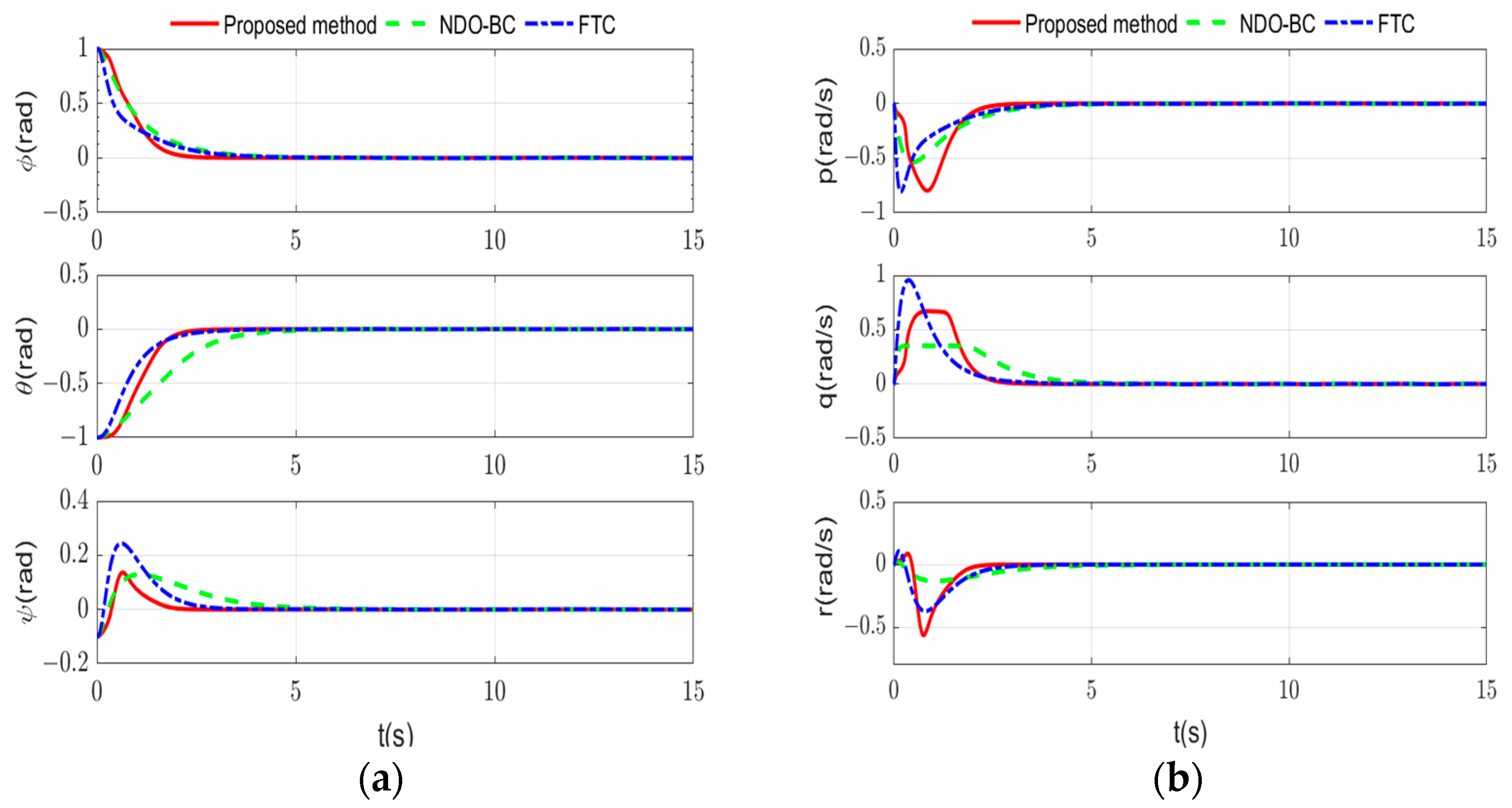
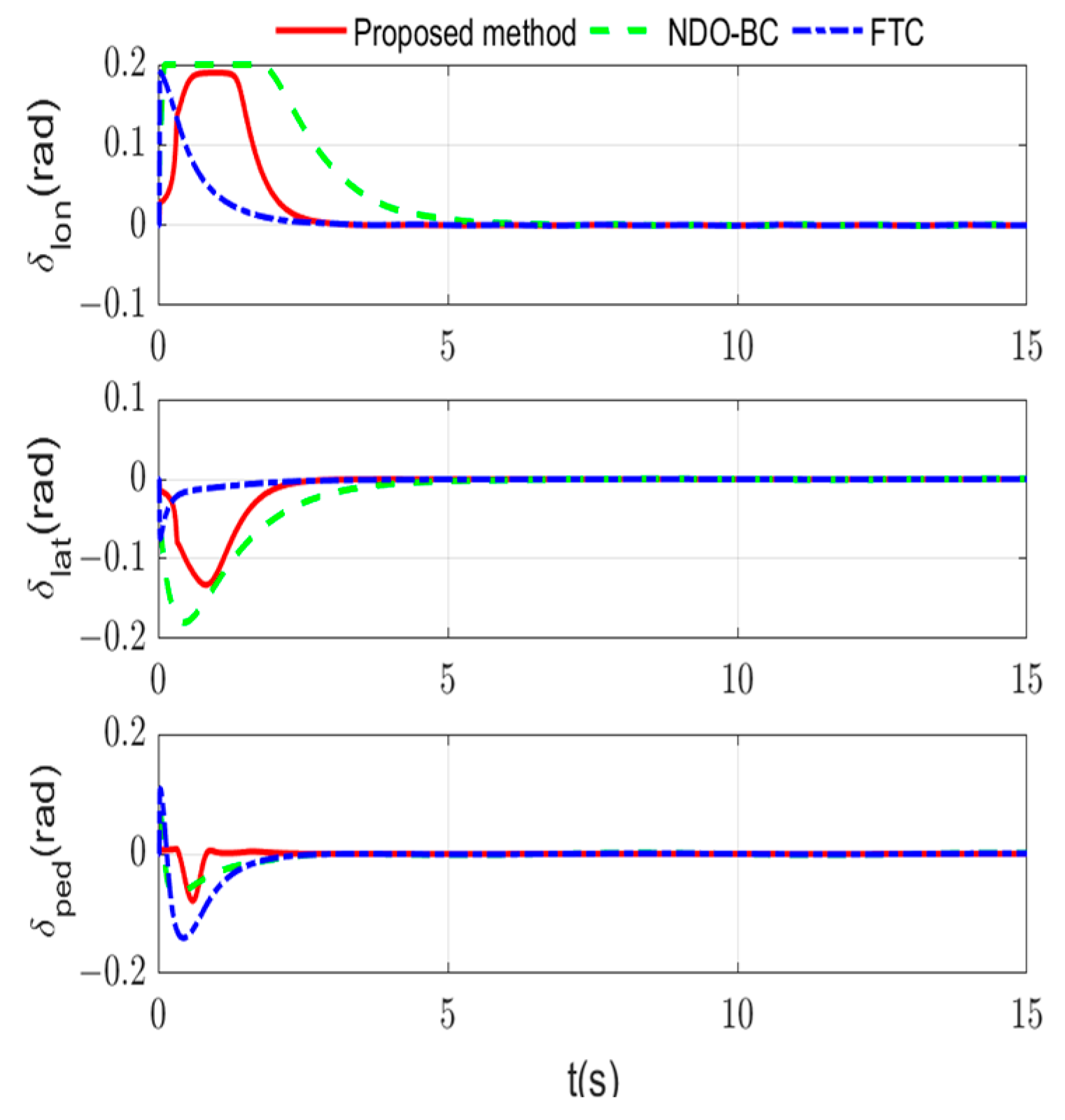
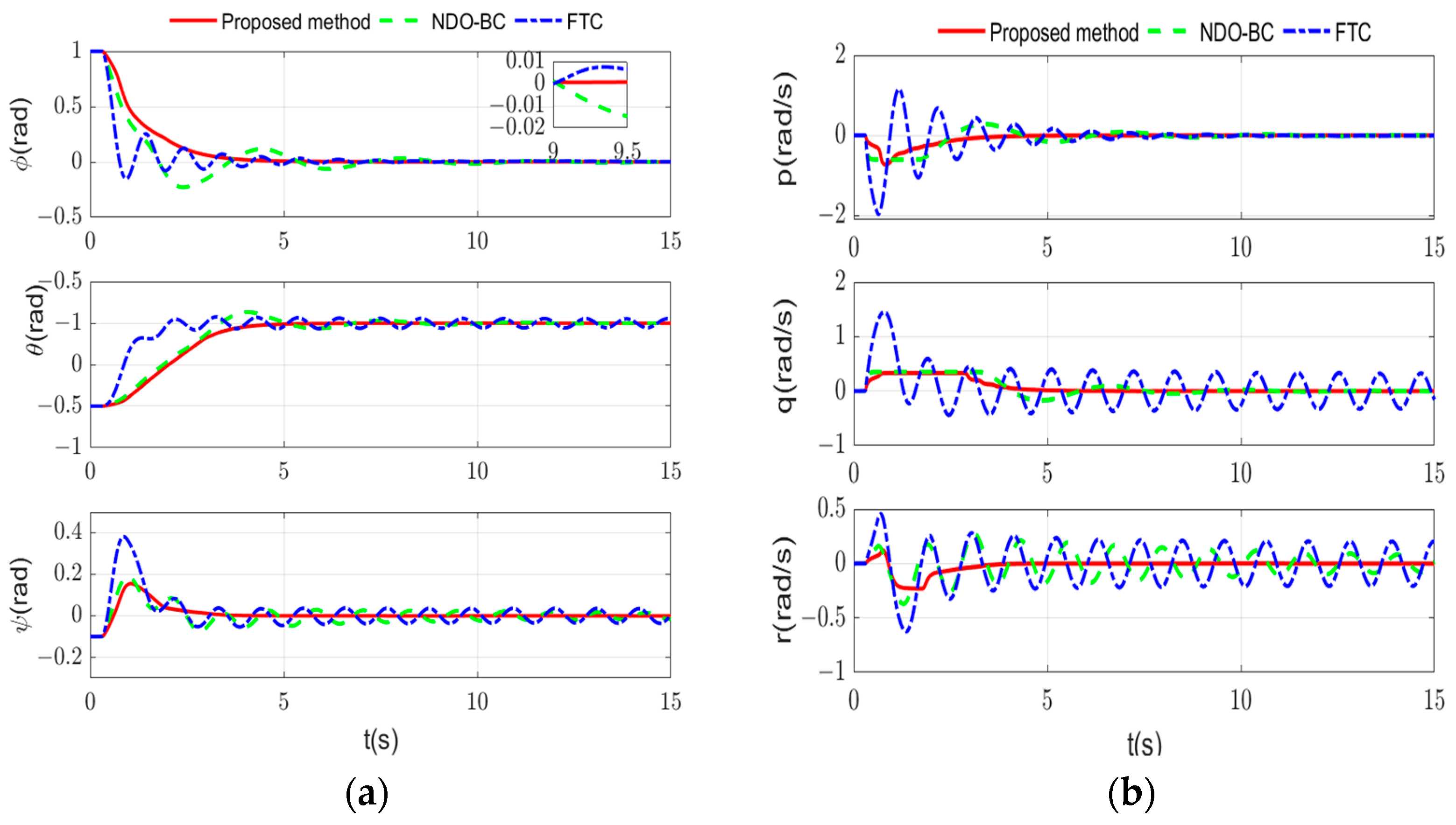
4. Simulation Results

Consider the UH attitude system in Equation (1). The model parameters given refer to [3,13]. The initial states are randomly set by ${\Theta }_0=[1,-1,0]$ rad and ${\Omega }_0=[0,0,0]$ rad/s. The input delay is assumed as $\tau ={\tau }_0+0.01*\sin (t)$, where ${\tau }_0=0.02$. The external disturbances are assumed as $d\left(t\right)=0.1*{[\cos (t)-3\sin (t),2\sin (4t)+\cos (2t),\cos (3t+\pi /3)]}^T$. The input saturation constraints and the attitude constraints are set as $u_{Mi}=0.2$, ${\delta }_1={\delta }_2=1.1$ and ${\delta }_3=0.2$, respectively. According to Theorems 1 and 2, the observer and the controller gains are designed as $k_{\Theta }=5$, $\gamma =0.6$, $k_{o1}=k_{o2}=1$, ${\xi }_o=a_0=1$, ${\varsigma }_o=\varsigma =0.01$, $u_{mi}=0.19$, ${\kappa }_1=1$, ${\kappa }_2=0.5$, ${\sigma }_1={\sigma }_2=1$, ${\gamma }_{c1}={\gamma }_{c2}={\gamma }_{c3}=1$ and ${\mu }_c=0.03$.

The attitude and angular velocity responses are shown in Figure 2. It can be seen that the attitude system converges to a small region containing zero with a settling time less than 4 s, and the steady accuracy is within ${10}^{-3}$. Moreover, the attitude angles are always confined within the constrained boundaries ${\delta }_i, i=1,2,3$. The curves of the adaptive parameters ${\xi }_c$ and ${\vartheta }_c$ are given in Figure 3, which converge to the equilibrium point in finite time. Thus, the finite-time stabilization of the attitude system is achieved in the presence of attitude constraints, input saturation, input delay and external disturbances.

The observed results of AFNO are shown in Figure 4. The observer states $\hat{S}$ and $\hat{d}$ can achieve rapid and accurate tracking of the actual variables of $S$ and $\overline{d}$, which indicates that AFNO can estimate the lump disturbances in finite time well. Moreover, it can be seen that the sliding mode surface converges to zero in finite time, and no chattering occurs in the approaching process. The commanded control inputs are shown in Figure 5, which are smooth and strictly within the saturation boundary 0.2.

To further illustrate the control performance of the proposed method, two controllers presented in [30] (noted as NDO-BC) and [17] (noted as FTC) are also applied to conduct the comparisons. The estimation results of the NDO and proposed AFBO observers are shown in Figure 6. It can be seen that the proposed AFNO has a faster convergence rate and higher estimation accuracy than the NDO. The comparison of the state responses under $\tau =0.2$ s is depicted in Figure 7. Although the other two schemes can achieve the attitude stabilization, the NDO-BC converges slowly, and the yaw angle $\psi$ under FTC has exceeded the attitude constraint ${\delta }_3$. The proposed controller has a faster convergence speed with better transient and steady-state performance under the attitude constraints. The comparison of the control input signals is shown in Figure 8. It can be observed that the other two methods consume larger control energy and suffer from saturation, while the proposed controller never violates the saturation constraint. In addition, in order to show the strong robustness of the proposed method, the compared results of the three methods under larger-scale input delay $\tau =0.3$ s are shown in Figure 9 and Figure 10. From the curves of simulations, one can see that the attitude convergence time under the proposed method is less than 4 s, and the steady-state error accuracy is less than ${10}^{-3}$, while the convergence time under the compared methods is more than 7 s, and the maximum steady-state error is about 0.02. Therefore, with the increase in input delay, the other two controllers show poorer transient characteristics, slower convergence rate, poorer steady-state accuracy and require larger control energy, while the proposed method can still ensure the fine stability of the control system and drive the states to the equilibrium point in finite time, consuming less control effort and showing strong robustness. All in all, the proposed control scheme can significantly achieve better control performance, which is concise, feasible and superior.

5. Conclusions

In this paper, a novel adaptive finite-time constrained attitude controller is investigated for the attitude stabilization of a UH system. Combining the BLF function and input memory compensation, a constrained memory sliding mode is first presented to deal with the attitude constraints and input delay. With the estimated disturbances by an adaptive finite-time nonlinear observer, a saturated finite-time attitude stabilization controller is designed to tackle the input saturation problem via the adaptive laws. Using Lyapunov synthesis, the finite-time stability of the closed-loop constrained attitude system is proven with all the signals bounded. Based on the proposed control scheme, the constrained attitude can converge to a small region with the settling time less than 4 s and the steady accuracy within ${10}^{-3}$ despite the disturbances, input delay and actuator saturation. Simulations have illustrated the effectiveness and superiority of the proposed method. In the future, the proposed scheme can further consider the problems of sensor failure and actuator stuck fault.

References

1. Aslam, F.; Haydar, M.F. H∞ inverse optimal attitude tracking on the special orthogonal group SO (3). Int. J. Control. 2023, 96, 3155–3167. [Google Scholar] [CrossRef]
2. Xie, S.; Chen, Q.; He, X.; Tao, M.; Tao, L. Finite-time command-filtered approximation-free attitude tracking control of rigid spacecraft. Nonlinear Dyn. 2022, 107, 2391–2405. [Google Scholar] [CrossRef]
3. Fang, X.; Wu, A.; Shang, Y.; Dong, N. A novel sliding mode controller for small-scale unmanned helicopters with mismatched disturbance. Nonlinear Dyn. 2016, 83, 1053–1068. [Google Scholar] [CrossRef]
4. Zheng, F.; Xiong, B.; Zhang, J.; Zhen, Z.; Wang, F. Improved neural network adaptive control for compound helicopter with uncertain cross-coupling in multimodal maneuver. Nonlinear Dyn. 2022, 108, 3505–3528. [Google Scholar] [CrossRef]
5. Gao, J.; Min, B.; Chen, Y.; Jing, A.; Wang, J.; Pan, G. Compound learning based event-triggered adaptive attitude control for underwater gliders with actuator saturation and faults. Ocean Eng. 2023, 280, 114651. [Google Scholar] [CrossRef]
6. Wang, Y.; Liang, T.; Yang, J.; Liu, J. Neuro-adaptive finite time composite fault tolerant control for attitude control systems of satellites. Radio Sci. 2024, 59, e2023RS007744. [Google Scholar] [CrossRef]
7. Canciello, G.; Cavallo, A.; D’Amato, E.; Mattei, M. Attitude and velocity high-gain control of a tilt-trirotor UAV. In Proceedings of the 2017 International Conference on Unmanned Aircraft Systems (ICUAS), Miami, FL, USA, 13–16 June 2017. [Google Scholar] [CrossRef]
8. Canciello, G.; Cavallo, A.; Schiavo, A.L.; Russo, A. Multi-objective adaptive sliding manifold control for More Electric Aircraft. ISA Trans. 2020, 107, 316–328. [Google Scholar] [CrossRef]
9. Islam, S.; Liu, P.X.; El Saddik, A. Robust control of four-rotor unmanned aerial vehicle with disturbance uncertainty. IEEE Trans. Ind. Electron. 2014, 62, 1563–1571. [Google Scholar] [CrossRef]
10. Zhou, B. Multi-variable adaptive high-order sliding mode quasi-optimal control with adjustable convergence rate for unmanned helicopters subject to parametric and external uncertainties. Nonlinear Dyn. 2022, 108, 3671–3692. [Google Scholar] [CrossRef]
11. Chen, W.H.; Yang, J.; Guo, L.; Li, S. Disturbance-observer-based control and related methods—An overview. IEEE Trans. Ind. Electron. 2016, 63, 1083–1095. [Google Scholar] [CrossRef]
12. He, W.; Yan, Z.; Sun, C.; Chen, Y. Adaptive neural network control of a flapping wing micro aerial vehicle with disturbance observer. IEEE Trans. Cybern. 2017, 47, 3452–3465. [Google Scholar] [CrossRef]
13. Wang, D.; Zong, Q.; Tian, B.; Shao, S.; Zhang, X.; Zhao, X. Neural network disturbance observer-based distributed finite-time formation tracking control for multiple unmanned helicopters. ISA Trans. 2018, 73, 208–226. [Google Scholar] [CrossRef]
14. Sabbghian-Bidgoli, F.; Farrokhi, M. Polynomial fuzzy observer-based integrated fault estimation and fault-tolerant control with uncertainty and disturbance. IEEE Trans. Fuzzy Syst. 2020, 30, 741–754. [Google Scholar] [CrossRef]
15. Chen, M.; Chen, W.H. Sliding mode control for a class of uncertain nonlinear system based on disturbance observer. Int. J. Adapt. Control Signal Process. 2010, 24, 51–64. [Google Scholar] [CrossRef]
16. Wu, S.N.; Sun, X.Y.; Sun, Z.W.; Wu, X.D. Sliding mode control for staring mode space craft using a disturbance observer. Proc. Inst. Mech. Eng. Part G J. Aerosp. Eng. 2010, 224, 215–224. [Google Scholar] [CrossRef]
17. Hu, Q.; Li, B.; Qi, J. Disturbance observer based finite-time attitude control for rigid spacecraft under input saturation. Aerosp. Sci. Technol. 2014, 39, 13–21. [Google Scholar] [CrossRef]
18. Cui, R.H.; Xue, X.J. Output feedback stabilization of stochastic planar nonlinear systems with output constraint. Automatica 2022, 143, 110471. [Google Scholar] [CrossRef]
19. Yang, Q.; Liu, H.; Yu, X.; Zhang, W.; Chen, J. Attitude constraint-based recovery for under-actuated AUVs under vertical plane control during the capture stage. Ocean Eng. 2023, 281, 115012. [Google Scholar] [CrossRef]
20. Mirshamsi, A.; Nobakhti, A. Uncertainty disturbance estimator control for delayed linear systems with input constraint. Automatica 2024, 167, 111763. [Google Scholar] [CrossRef]
21. Tee, K.P.; Ge, S.S.; Tay, E.H. Barrier Lyapunov functions for the control of output-constrained nonlinear systems. Automatica 2009, 45, 918–927. [Google Scholar] [CrossRef]
22. Tee, K.P.; Ge, S.S. Control of nonlinear systems with partial state constraints using a barrier Lyapunov function. Int. J. Control. 2011, 84, 2008–2023. [Google Scholar] [CrossRef]
23. Li, R.; Chen, M.; Wu, Q. Adaptive neural tracking control for uncertain nonlinear systems with input and output constraints using disturbance observer. Neurocomputing 2017, 235, 27–37. [Google Scholar] [CrossRef]
24. Yan, K.; Chen, M.; Wu, Q.; Zhu, R. Robust adaptive compensation control for unmanned autonomous helicopter with input saturation and actuator faults. Chin. J. Aeronaut. 2019, 32, 2299–2310. [Google Scholar] [CrossRef]
25. Chen, M.; Zhou, Y.; Guo, W.W. Robust tracking control for uncertain MIMO nonlinear systems with input saturation using RWNNDO. Neurocomputing 2014, 144, 436–447. [Google Scholar] [CrossRef]
26. Chu, Z.; Xiang, X.; Zhu, D.; Luo, C.; Xie, D. Adaptive fuzzy sliding mode diving control for autonomous underwater vehicle with input constraint. Int. J. Fuzzy Syst. 2018, 20, 1460–1469. [Google Scholar] [CrossRef]
27. Wang, M.; Zhang, T. Leader-following formation control of second-order nonlinear systems with time-varying communication delay. Int. J. Control Autom. Syst. 2021, 19, 1729–1739. [Google Scholar] [CrossRef]
28. Yang, H.L.; Ruby, R.; Wu, K.S. Delay performance of priority-queue equipped UAV-based mobile relay networks: Exploring the impact of trajectories. Comput. Netw. 2022, 210, 108856. [Google Scholar] [CrossRef]
29. Zhou, J.; Wen, C.; Wang, W. Adaptive backstepping control of uncertain systems with unknown input time-delay. Automatica 2009, 45, 1415–1422. [Google Scholar] [CrossRef]
30. Li, S.; Duan, N.; Min, H. Trajectory tracking control for quadrotor unmanned aerial vehicle with input delay and disturbances. Asian J. Control. 2024, 26, 150–161. [Google Scholar] [CrossRef]
31. Li, D.P.; Liu, Y.J.; Tong, S.; Chen, C.P.; Li, D.J. Neural networks-based adaptive control for nonlinear state constrained systems with input delay. IEEE Trans. Cybern. 2018, 49, 1249–1258. [Google Scholar] [CrossRef]
32. You, F.; Chen, N.; Zhu, Z.; Cheng, S.; Yang, H.; Jia, M. Adaptive fuzzy control for nonlinear state constrained systems with input delay and unknown control coefficients. IEEE Access 2019, 7, 53718–53730. [Google Scholar] [CrossRef]
33. Luo, R.C.; Chung, L.Y. Stabilization for linear uncertain system with time latency. IEEE Trans. Ind. Electron. 2002, 49, 905–910. [Google Scholar] [CrossRef]
34. Yue, D.; Han, Q.L. Delayed feedback control of uncertain systems with time-varying input delay. Automatica 2005, 41, 233–240. [Google Scholar] [CrossRef]
35. Tong, S.; Sui, S.; Li, Y. Fuzzy adaptive output feedback control of MIMO nonlinear systems with partial tracking errors constrained. IEEE Trans. Fuzzy Syst. 2015, 23, 729–742. [Google Scholar] [CrossRef]
36. Yu, J.; Shi, P.; Zhao, L. Finite-time command filtered backstepping control for a class of nonlinear systems. Automatica 2018, 92, 173–180. [Google Scholar] [CrossRef]
37. Wang, X.; Wang, Q.; Sun, C. Adaptive tracking control of high-order MIMO nonlinear systems with prescribed performance. Front. Inf. Technol. Electron. Eng. 2021, 22, 986–1001. [Google Scholar] [CrossRef]
38. Ye, D.; Xiao, Y.; Sun, Z.; Xiao, B. Neural network based finite-time attitude tracking control of spacecraft with angular velocity sensor failures and actuator saturation. IEEE Trans. Ind. Electron. 2021, 69, 4129–4136. [Google Scholar] [CrossRef]
39. Zhu, Z.; Xia, Y.; Fu, M. Attitude stabilization of rigid spacecraft with finite-time convergence. Int. J. Robust Nonlinear Control. 2011, 21, 686–702. [Google Scholar] [CrossRef]
40. Bhat, S.P.; Bernstein, D.S. Finite-time stability of continuous autonomous systems. SIAM J. Control Optim. 2000, 38, 751–766. [Google Scholar] [CrossRef]
Figure 1. Overview of the attitude control architecture.
Processes 12 01787 g001
Figure 2. States responses. (a) Attitude curves with constraints; (b) angular velocity curves.
Processes 12 01787 g002
Figure 3. Adaptive parameter curves.
Processes 12 01787 g003
Figure 4. Estimations of AFNO. (a) Estimation of S ; (b) estimation of d ¯ .
Processes 12 01787 g004
Figure 5. Control input curves.
Processes 12 01787 g005
Figure 6. Observation results. (a) Estimation of d ¯ ; (b) estimation error d ˜ .
Processes 12 01787 g006
Figure 7. State response comparison under a delay of 0.02 s. (a) Attitude curves; (b) angular velocity curves.
Processes 12 01787 g007
Figure 8. Control input comparison under a delay of 0.02 s.
Processes 12 01787 g008
Figure 9. State response comparison under a delay of 0.3 s. (a) Attitude curves; (b) angular velocity curves.
Processes 12 01787 g009
Figure 10. Control input comparison under a delay of 0.3 s.
Processes 12 01787 g010
Disclaimer/Publisher’s Note: The statements, opinions and data contained in all publications are solely those of the individual author(s) and contributor(s) and not of MDPI and/or the editor(s). MDPI and/or the editor(s) disclaim responsibility for any injury to people or property resulting from any ideas, methods, instructions or products referred to in the content.