RUL Prediction of Rolling Bearings Based on Multi-Information Fusion and Autoencoder Modeling

Abstract

As an important part of industrial equipment, the safe and stable operation of rolling bearings is an important guarantee for the performance of mechanical equipment. Aiming at the problem that it is difficult to characterize the running state of rolling bearings, this paper mainly analyzes and processes the vibration signals of rolling bearings, extracts and fuses multi-information entropy, and monitors the running state of rolling bearings and predicts the remaining useful life prediction (RUL) through test verification. Firstly, in view of the difficulty in characterizing the bearings running state characteristics, a rolling bearings running state monitoring method based on multi-information entropy fusion and denoising autoencoder (DAE) was proposed to extract the multi-entropy index features of vibration signals to improve the accuracy of feature extraction, and to solve the problem of not obvious information representation of a single feature indicator and missing information in the feature screening process. Secondly, in view of the problems of low prediction accuracy and poor robustness and generalization in traditional RUL models, a rolling bearings RUL model combining convolutional autoencoder (CAE) and bidirectional long short-term memory network (BiLSTM) was proposed. The introduction of convolution operation made CAE have the feature of weight sharing, reducing the complexity of the model. Finally, the XJTU-SY data set was used to verify the constructed model. The results show that the condition monitoring model established in this paper can accurately evaluate the running state of the rolling bearing and accurately locate the failure time. At the same time, the residual life prediction model can realize the residual life prediction of most data sets, and has good accuracy and robustness.

1. Introduction

With the rapid development of intelligent manufacturing, the running performance of rolling bearings, as one of the important parts of rotating machinery and equipment, plays a crucial role in the overall operation of the system [1], so it is of great significance to monitor the running condition of rolling bearings and predict their remaining life.

In actual working conditions, the bearing is in a nonlinear system and interfered environment. In the process of signal collection, the environment is complex and changeable, presenting non-stationary characteristics, which increases the difficulty of operation state monitoring [2]. At present, due to the easy acquisition of vibration signals and the fact that vibration signals can more directly reflect the running state of bearings, they are widely used in bearing feature extraction [3]. Through feature fusion of time–frequency domain information extraction and a combination of vibration signals, the running state monitoring of rolling bearings has been realized [4,5]. Zheng et al. [6] proposed a rolling bearing feature extraction method based on optimized variational mode decomposition and used the kurtosis criterion to perform envelope demodulation on decomposed IMF components and extract bearing operating features. The feature parameters extracted by the above methods do not reveal the characteristics of changes in the potential state of the system. In recent years, the entropy weight method has been applied more and more widely in the field of feature extraction, which can accurately express the degree of internal information disorder of the system with low degradation feature dimension. Wang et al. [7] built a feature-level fusion algorithm based on association entropy to make full use of the extracted signal degradation feature information in fault prediction. With the constant development of intelligent industry and information technology in recent years, as well as the advance of computer technology, data-driven and intelligent algorithms with the combination of technology are widely applied in the field of condition monitoring and prediction, and have made a lot of progress [8]. Autoencoder (AE) is an unsupervised learning model [9], which is generally composed of an encoder and a decoder. Since it was proposed in 2006, AE has received much attention in the field of machine learning and has achieved significant applications in many fields. Tao et al. [10] made some improvements to AE and successfully applied it in the fault diagnosis of equipment and bearings, showing the capability of AE in feature extraction and classification. On this basis, Wang et al. [11] combined the kernel function with DAE, which not only improved the effect of feature extraction, but also improved the ability of model fault diagnosis.

Recurrent neural network (RNN) is widely used in time series prediction because it can capture the time dependence in the series and effectively use historical information to predict future results [12]. Jiao et al. [13] made full use of the extracted coarse-grained fine-grained features to estimate health index (HI), proposed a new deep learning network architecture based on RNN, and estimated the probability distribution of RUL by extrapolating the HI degradation model to a predefined fault threshold. Long short-term memory network (LSTM) improves the performance and stability of the model by introducing a cell state and gating mechanism [14]. Wang et al. [15] introduced the CAE enhanced by the whole life cycle mechanism and the LSTM enhanced by the bias correction mechanism to reduce the influence of the large concavity of the input HI on the prediction model. In order to make up for the limitation that the traditional LSTM still follows the unidirectional propagation from front to back in the processing of time series, the proposal of BiLSTM can effectively combine the forward and backward time series information, thereby improving the processing ability of the model on time series data [3], and it has been successfully applied to RUL prediction [16,17].

Based on the above analysis, in view of the problems that a single running feature is difficult to accurately characterize the running state, the prediction effect of RUL model is poor, and the prediction time is long, this paper adopts multi-entropy fusion and deep learning methods to predict the remaining life of rolling bearings. The main research contents are as follows:

• In view of the problem that it is difficult to accurately characterize the running state with a single running feature, multi-information entropy feature extraction is carried out for vibration signals, and multi-entropy indicators are used to improve the characterization ability and provide a basis for the subsequent construction of HI.
• At present, the extracted feature indicators in some studies have too much information, which belongs to high-dimensional feature information, excessive redundant information, and difficult screening. In traditional feature use, it is easy to cause the omission of important feature information or the calculation time is too long, and it is difficult to ensure the accuracy and overall feature extraction. In this paper, DAE was used for multi-information entropy fusion and dimensionality reduction, HI was constructed to evaluate the running state of bearings, and significant root mean square (RMS) value jump time was found as the failure threshold of HI to evaluate the running state of bearings.
• Aiming at the problem of large amounts of calculation and time required when LSTM deals with long sequence problems, the powerful feature extraction ability of CAE is used to extract the unsupervised features of vibration signals, and the hidden features are input into BiLSTM for RUL prediction.

2. Theoretical Backgrounds

2.1. Denoising Autoencoder

DAE is a kind of unsupervised neural network that contains hidden features and mainly consists of an input layer, processing layer, hidden layer, and reconstruction layer. Its basic model is shown in Figure 1, where x_i represents the input raw data and y_i is the dimensionality reduction data obtained through coding learning.

The core ideas of DAE are as follows. Given a training sample set N, for each input original data x (x∈N), it is denoised according to the q_D distribution. This process is to clear nodes of some dimensions with a certain probability, and then use these data after node zeroing for training. Through this process, feature y reduced to t-dimension is learned. Using these features y, the original k-dimension input data $\widehat{x}$ are reconstructed. In the whole training process, DAE adjusts the model parameters to obtain the minimum loss function, so as to achieve the optimization of the model.

For sample set N, the minimization loss function J of DAE can be expressed as:

$$J={\displaystyle \sum _{x\in N}}L\left(x,\widehat{x}\right)$$

(1)

where x is the input raw data, $\widehat{x}$ is to reconstruct sample data, and $L\left(x,\widehat{x}\right)$ is the reconstruction error of a single sample.

$L\left(x,\widehat{x}\right)$ can be expressed by calculating the mean square error between the input layer and the reconstructed layer, and the formula is as follows:

$$L\left(x,\widehat{x}\right)={\displaystyle \frac{1}{k}}{\displaystyle \sum _{i=1}^k}\left(x_i-{\widehat{x}}_i\right)$$

(2)

Under the learning condition of reconstruction error optimization, the internal mapping of DAE has strong robustness, which significantly reduces the sensitivity of the model to small random perturbations. This enables DAE not only to effectively reduce the dimensionality of data, but also to have certain noise reduction capabilities, thus improving the stability and performance of the model [18].

2.2. Convolutional Autoencoder

In the network structure parameters of AE, with the increase in the number of network layers, the number of hyperparameters will increase, which will increase the overall training difficulty of AE, and the data effect of decoder reconstruction is poor. Due to the weight-sharing principle, convolutional neural networks (CNN) significantly reduce the number of weights and biases, thus reducing the complexity of model parameters [19]. Based on the structure idea of AE, CAE is constructed by cleverly integrating convolution operations and pooling layer operations in CNN into AE.

CAE no longer uses a fully connected layer during encoding and decoding, but instead uses convolution operations [20]. Through the convolution operation, the hidden layer is extracted from the output layer to complete the convolution encoding. The decoder uses the deconvolution operation to reconstruct the hidden layer to obtain the output layer with the same dimension as the input layer and complete the convolution decoding. The error between the output layer and the input layer is calculated, and after several iterations until the error reaches the minimum, the network parameters of CAE are obtained. The structure diagram of CAE is shown in Figure 2.

The analysis of Figure 2 shows that the fully connected structure of CAE is different from AE. In CAE, neurons in each layer are only connected with some neurons in the upper layer. For example, neuron n₂ only forms connections with neurons m₁, m₂, and m₃ in the upper layer. This design makes CAE pay more attention to local learning ability in data processing. By introducing convolution operations in CNN, CAE not only reduces the complexity of model parameters, but also effectively obtains the feature map of data by moving each convolution kernel in an orderly way. At the same time, the weight-sharing mechanism enables CAE to monitor and recognize the same local features of different location features in the network. This feature enables CAE to extract the translation invariant characteristics of data in the analysis of bearing vibration signals, thus greatly enhancing the capability of feature capture.

2.3. Bidirectional Long Short Term Memory Network

Although LSTM network successfully solved the problems existing in the RNN network, in the process of network training and learning, the traditional LSTM still follows the principle of one-way propagation from front to back in the processing of time series. This one-way propagation method is not effective in the processing of time series data, and it cannot use the backward propagation information from back to front. To compensate for this limitation, BiLSTM is proposed, which can effectively combine forward and backward time series information. Thus, the processing capability of the model on time series data is improved [3].

The network structure of BiLSTM is shown in Figure 3. In this structure, LSTM along the positive direction of time series can store the history information of input sequence data in sequence. The LSTM in the opposite direction of the time series can store the future information of the input sequence data in reverse order. Two LSTMs in opposite directions of the time series are finally connected to an output layer, and the hidden layer between the two LSTMs is also connected. This design effectively avoids the information exchange between the two time series, thus ensuring that the information in both directions can be fully utilized when processing time series data.

The hidden layer state of each level of BiLSTM is calculated as follows:

$$\begin{array}{l}{h}_t=\mathrm{LSTM}\left(x_t,h_{t-1}\right)\\ h_i=\mathrm{LSTM}\left(x_t,h_{i-1}\right)\\ h_t^{\prime }=a_t{h}_t+b_t{h}_i+o_t\end{array}$$

(3)

where h_t and h_i represent the state of the hidden layer during forward transmission and reverse transmission, respectively; $h_t^{\prime }$ indicates the state of each hidden layer; a_t and b_t represent the calculated weights of forward and reverse transmission, respectively; o_t indicates calculation bias.

2.4. Multi-Information Selection Indicator

Entropy is a thermophysical concept used to characterize the amount of information. In recent years, many experts and scholars have introduced entropy features into the field of feature extraction to realize the datalization of operating states by calculating various entropy values of vibration signals. As a dimensionless index to characterize the complexity of time series, the greater the entropy value, the greater the disorder complexity of the signal. In this paper, relative entropy (ReEn) [21], approximate entropy (ApEn) [22], permutation entropy (PmEn) [23], fuzzy entropy (FuEn) [24], discrete entropy (DisEn) [25], and symbolic dynamic entropy (SDEn) [26,27] are selected as the characteristic indexes of multi-information fusion.

2.5. Health Index Construction Method

Using the excellent feature fusion and dimensionality reduction capabilities of DAE, the purpose of eliminating small redundant features and dimensionality reduction of feature indexes is realized. HI is constructed in two stages, offline and online. In the offline stage, encoders that can extract features effectively are obtained by training the model and the minimum loss function. The online phase builds the HI using the already trained model. The construction process of HI is shown in Figure 4.

The specific steps to obtain HI in the offline phase are as follows:

(1)

Bearing lifetime vibration acceleration signal is obtained through bearing data set.

(2)

Take the first 2048 frequency points of each data set as the training samples of the model.

(3)

The characteristic indexes of ReEn, ApEn, PeEn, FuEn, DisEn, and SDEn are calculated for the intercepted training samples.

(4)

Adam was selected as the optimizer and the DAE was trained using the training set. The loss function was as follows:

$$L\left(\widehat{x},x\right)={\displaystyle \frac{1}{k}}{\displaystyle \sum _{i=1}^k}{\mathrm{smooth}}_{L1}\left(y^{\left(i\right)}-x^{\left(i\right)}\right)+\lambda {{\displaystyle \sum _{i=1}^q}‖w_i‖}_2^2$$

(4)

$${\mathrm{smooth}}_{L1}\left(z\right)=\left\{\begin{array}{ll}0.5z^2& z\ge 0\\ \left|z\right|-0.5& \mathrm{else}\end{array}\right.$$

(5)

where k is the number of feature samples contained in the input data, $y^{\left(i\right)}$ is the eigenvalue of the number i sample after the reconstruction of the characteristic sample, $x^{\left(i\right)}$ is the characteristic value of the number i sample of the input data, $\lambda$ is L2 regularization coefficient, m is the number of weights in the neural network, and $w_i$ is the number i weight in the neural network.

(5)

When the loss value stops falling, it can be judged that the training is complete, and an encoder capable of effectively extracting features and dimensionality reduction can be obtained.

The specific steps to obtain HI in the online phase are as follows:

(1)

The data at the initial moment of the data set are stacked after multi-entropy feature index calculation, and input into the trained DAE to obtain the bearing characteristics in the health state.

(2)

Calculate the multi-entropy feature indicators of the data at the current time, and also input these indicators into the trained DAE to obtain the degraded state characteristics of the bearing under the current state.

(3)

Calculate the Bray–Curtis distance between the health state feature and the degraded state feature [28], and take these index data as the running state HI of the bearing.

The value range of Bray–Curtis distance is between 0 and 1. When the indicator data point is closer to 0, it indicates that the difference between the two features is smaller, thus reflecting the healthier operation of the bearing. On the contrary, when the data point is closer to 1, it means that the difference between the two features is greater, indicating that the bearing is gradually approaching the failure state. The specific calculation method is as follows:

$$D_{pq}={\displaystyle \sum _{k=1}^n}\left|x_{pk}-x_{qk}\right|/({\displaystyle \sum _{k=1}^n}{x}_{pk}+{\displaystyle \sum _{k=1}^n}{x}_{qk})$$

(6)

where $x_{pk}$ is the number k feature under the health status feature; $x_{qk}$ is the number k feature under the degenerate state feature.

2.6. Failure Threshold Construction Method

The selection of the failure threshold of HI has always been a crucial part of Prognostic and Health Management problems. For the HI values established in this section, especially those without clear physical meaning, there is no standard to determine their failure threshold [29]. Therefore, in many studies, it is assumed that the RMS value of data samples can reflect the degree of degradation of rolling bearings, and the significant amplitude jump of RMS is considered to be the moment of state change of bearing life [30], and the growth is very rapid at this time, as shown by the actual trend. In this section, the RMS jump time is taken as the state change time of the bearing, and the amplitude of HI at this time is taken as the failure threshold of the bearing.

According to the above, the time when the RMS jumps to 4 times the normal value is regarded as the failure time, and the HI value at this time is the failure threshold. In order to reduce the interference of redundant information on the model and improve the robustness, this section adopts a moving average filter to flatten the current HI value, with a window size of 5. The specific process is shown in Figure 5, and the specific steps are as follows:

(1)

Obtain the HI value of the current moment and then insert it into the HI sequence in chronological order.

(2)

In order to obtain a smoother HI sequence, the moving average filter is used to filter the current HI sequence.

(3)

Calculate the RMS value $X_{RMS}$ of the HI sequence at the current moment, and compare the HI value at the current moment with the failure threshold (4$X_{RMS}$); if the failure threshold is reached, the bearing has reached the degradation stage. Set the HI value at this time as the failure threshold of the bearing. The RMS calculation formula is as follows:

$$X_{RMS}=\sqrt{{\displaystyle \frac{1}{N}}{\displaystyle \sum _{i=1}^N}{x}_i^2}$$

(7)

where N is the number of HI samples at the current time; x_i is the current time HI value.

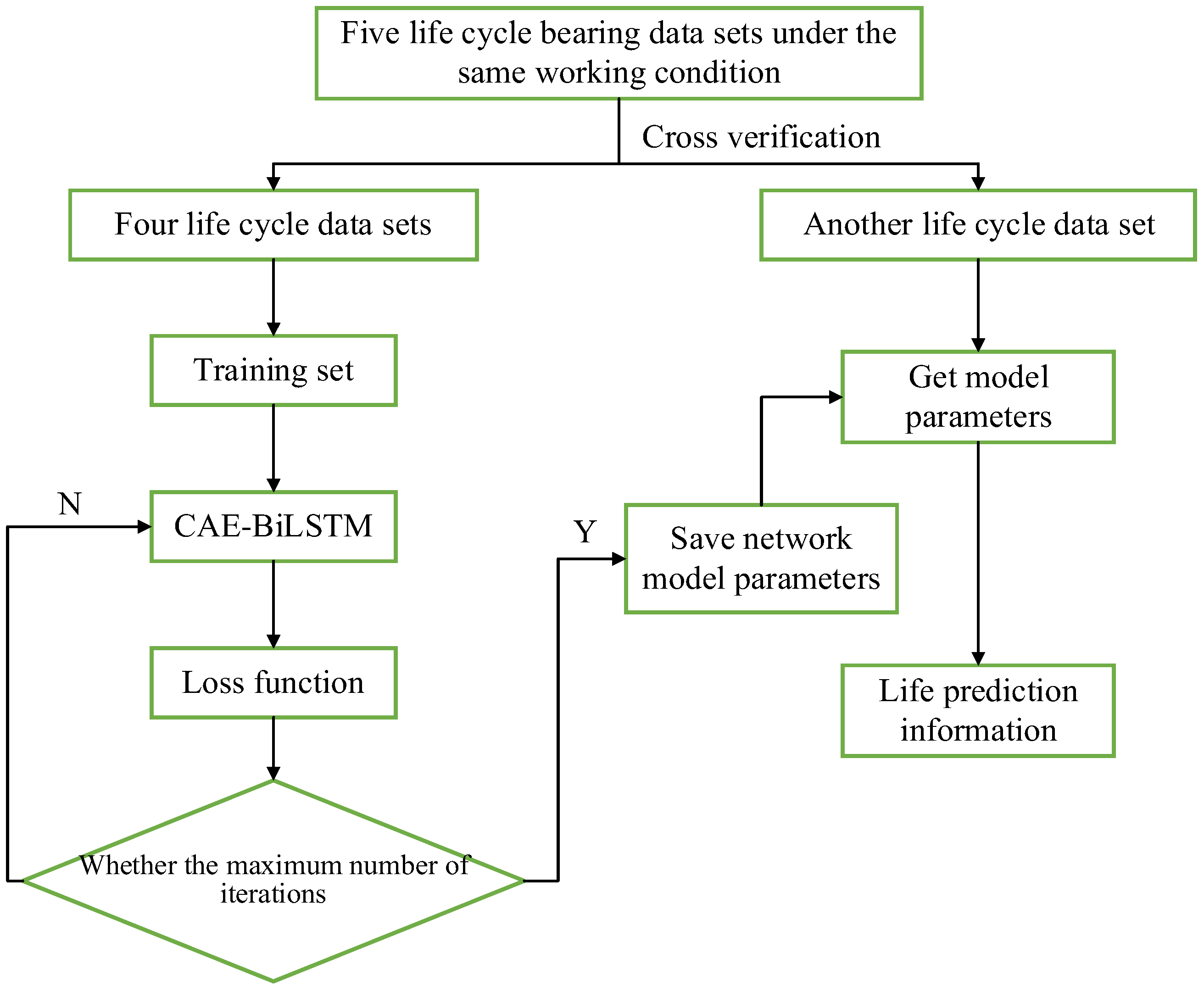
2.7. RUL Model Based on CAE-BiLSTM

The CAE-BiLSTM hybrid model of the RUL prediction method proposed in this paper is shown in Figure 6. Firstly, the CAE layer is used to learn the bearing degradation data features, and the BiLSTM network is used to learn the time-dependent features of vibration signals by considering future data information and combining all the information. Finally, the RUL prediction data are obtained by the fully connected layer.

The unsupervised RUL prediction model constructed in this paper includes three parts: data processing, model training, and RUL prediction. In the data processing stage, the original data are screened and normalized to ensure the quality and consistency of the data. In the model training stage, iteratively train the loss function and continuously optimize the network model to improve the performance of the model. After the network training is completed, the test samples are input into the trained CAE-BiLSTM model to achieve the prediction of bearing RUL. The flowchart is shown in Figure 7. The specific steps are as follows:

(1)

Firstly, the data are preprocessed, and after the data are normalized, the time domain data are converted into envelope spectrum data by Hilbert yellow transformation for model training.

(2)

Initialize the parameters of the CAE-BiLSTM network, process the data, adjust the input data according to the characteristics of the network model, and prepare to train the network. According to the test data, the remaining four data sets under the same working conditions are used as the training set.

(3)

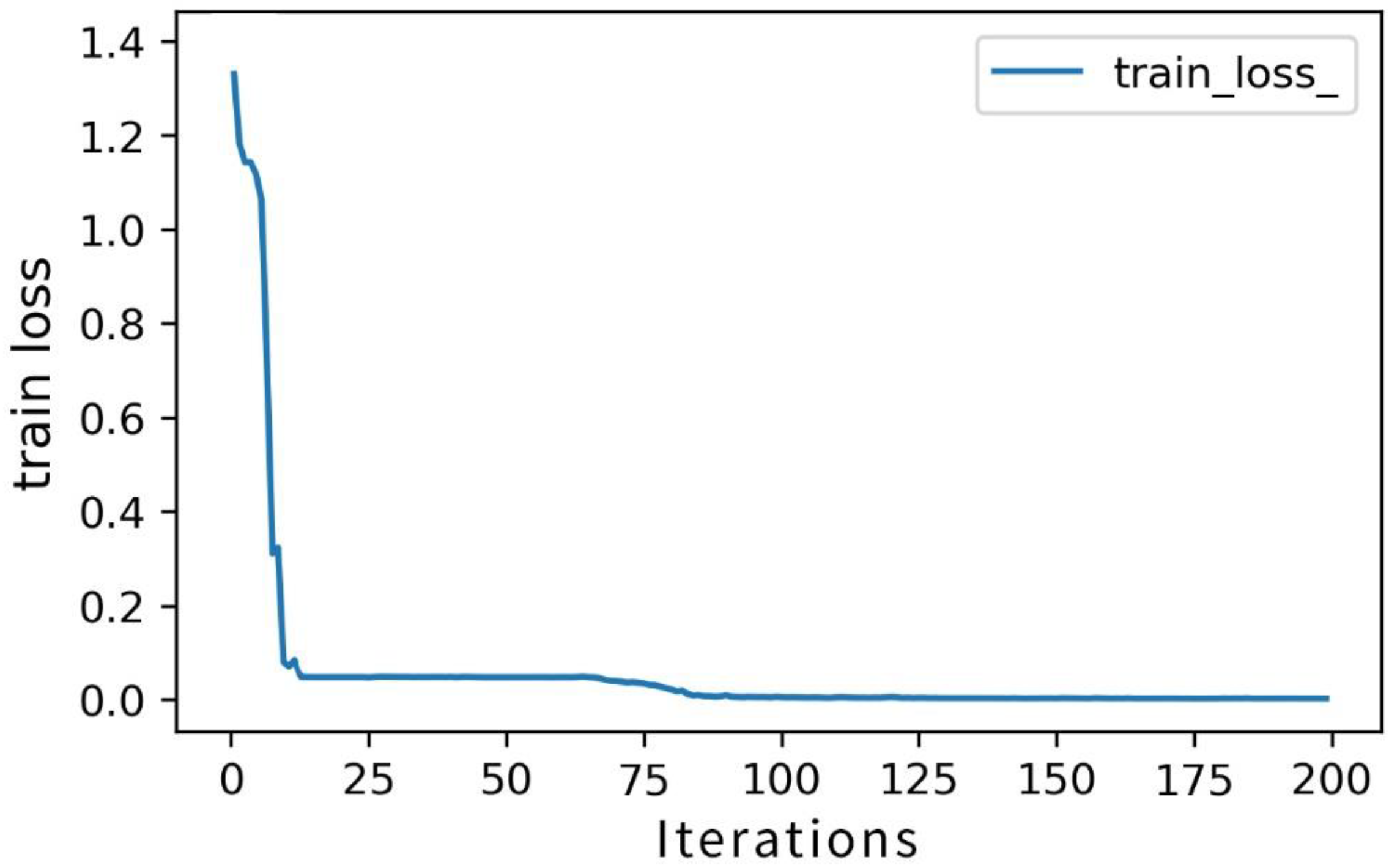
Conduct network training, construct loss function, calculate loss function value, and optimize the network through optimization algorithm.

(4)

Determine whether the maximum number of iterations is reached. If the maximum number of iterations is reached, the training is completed; otherwise, return to step (3).

(5)

Save the trained model parameters, input the test data into the trained CAE-BiLSTM network, and obtain the prediction results.

3. Results

3.1. Multi-Entropy Extraction Process

The bearing data set used in the test was derived from the full-life rolling bearing data set published by Xi’an Jiaotong University [31]. The equipment platform supported by the data set integrates key components such as an AC motor, motor speed controller, rotating shaft, support bearing, hydraulic loading system, and test bearing. The establishment of the test platform can conduct accelerated life tests for rolling bearings and plain bearings under different working conditions, and comprehensively collect data on test bearings during the whole life cycle [32]. The specific bearing model used in the test is the LDK UER204 rolling bearing. The whole data set covers three different working conditions, and there are four failure positions of inner ring, outer ring, cage, and rolling body. The specific information of the data set is shown in

Table 1. Specific information of bearing data set.

Working Condition	Data Set	Sample Count	Basic Rated Life	Actual Life	Fault Type
1	Bearing1_1	123	5.600–9.677 h	2 h 3 min	Outer ring
	Bearing1_2	161		2 h 41 min	Outer ring
	Bearing1_3	158		2 h 32 min	Outer ring
	Bearing1_4	122		2 h 2 min	Cage
	Bearing1_5	52		52 min	Outer ring, Inner ring
2	Bearing2_1	491	6.786–11.726 h	8 h 14 min	Inner ring
	Bearing2_2	161		2 h 41 min	Outer ring
	Bearing2_3	533		8 h 38 min	Cage
	Bearing2_4	339		5 h 39 min	Outer ring
	Bearing2_5	42		42 min	Outer ring
3	Bearing3_1	2538	8.468–14.632 h	42 h 18 min	Outer ring
	Bearing3_2	2496		41 h 36 min	Inner ring, Outer ring, Cage, rolling body
	Bearing3_3	371		6 h 11 min	Inner ring
	Bearing3_4	1515		25 h 15 min	Inner ring
	Bearing3_5	114		1 h 54 min	Outer ring

. In this paper, the experimental simulation validation based on Python v3.10 implementation, and invoke TensorFlow v2.9.0 deep learning framework.

Bearing1_1 and Bearing3_1 bearing data were selected to carry out multi-entropy feature extraction, and the time domain waveform diagram of bearing vibration signals throughout their life cycle was drawn, as shown in Figure 8.

According to Figure 8a, the amplitude of Bearing1_1 in the middle and back of the time domain signal gradually increases, indicating that the operating state of the bearing has changed. As shown in Figure 8b, Bearing3_1 has a large number of samples and is always in a state of high amplitude, so it is difficult to distinguish the specific running state of the bearing. Therefore, the next step is to extract the feature of the vibration signal.

The ReEn, ApEn, PmEn, FuEn, DisEn, and SDEn of each sample are calculated according to the number of samples divided by the bearing data set and the characteristic indexes introduced above. Figure 9 and Figure 10 show the multi-entropy feature extraction results of Bearing1_1 and Bearing3_1, respectively.

According to the analysis of Figure 9, Bearing1_1 has a total of 123 data sets, and six entropy values with the number of sample sequences of 123 are obtained through calculation. It can be seen from the change curve in Figure 9 that the time of data jump for each entropy value is different; for example, the ReEn, ApEn, and FuEn change after the 80th samples. The PmEn and SDEn complete the data jump before sample 80. From the perspective of thermal entropy, it indicates that chaos has occurred inside the bearing system when the data jump occurs, which proves that the running state of the bearing has changed.

According to the same analysis as shown in Figure 10, the entropy values of Bearing3_1 also changed before and after the 2390th sample, and the running state of the bearings changed. Because of the differences in the subtle features represented by each entropy, the HI value constructed by a single feature can reduce the calculation time, but there is a problem of incomplete feature extraction. Moreover, the extracted entropy does not change much before and after the jump time, so the use of multi-information fusion can enrich the constructed HI value feature quantity and improve the accuracy of the evaluation.

3.2. Construction of Health Indicator and Failure Threshold

In the training stage, the whole life cycle data of other bearings except test bearings under the same working conditions are used as the training set, so that the model can fully learn the operating characteristics of rolling bearings under the same working conditions. During the test phase, the life cycle data of Bearing1_1 and Bearing3_1 are used as test sets to evaluate the performance of the model. After completing the model training, build the HI and select the failure threshold.

In the offline training phase, set the batch size of model training to 50 and the number of iterations to 1000. For the optimizer, select the Adam optimizer and set the initial learning rate to 1 × 10⁻³. At the same time, in order to prevent overfitting, the regularization coefficient of L2 is introduced to be 1.2 × 10⁻⁵. After training, the loss curve is shown in Figure 11. It can be clearly seen from the figure that the convergence of the loss function is fast, only the 36th generation has converged to the lowest level, and the final loss value is stable at 1.05 × 10⁻³.

In the online test stage, the HI value and failure threshold of Bearing1_1 and Bearing3_1 are shown in Figure 12 and Figure 13. It can be seen from the curves in the figure that the HI after multi-entropy fusion presents good monotonicity, which is specifically shown as an increasing trend, showing the complete process from the initial degradation to the final complete failure of the bearing. In addition, the sudden increase in HI occurred during the running of the bearing. Based on the Bray–Curtis distance used in the method proposed in this section, it indicates that the bearings failed in the late running state.

According to the analysis of Figure 12, the HI value of Bearing1_1 in the 78th sample is 0.0715, and the HI value in the 79th sample is suddenly increased to 0.3836. When calculating the RMS value at this time, it is found that there has been a jump, so the HI value of the 78th sample is set as the failure threshold of the bearing. It should be noted that the HI value constructed in the 69th sample is 0.0713, which is close to the failure threshold, but the root mean square jump in the HI value of the next sample does not occur, and the operating state of the bearing cannot be determined to change.

Similarly, the HI value of Bearing3_1 in the 2380th sample was 0.0953, and the HI value of Bearing3_1 in the 2381st sample suddenly increased to 0.2646, and RMS jump also occurred. Therefore, the HI value of the 2381st sample 0.0953 was set as the failure threshold of the bearing. The single entropy feature index of Bearing3_1 extracted in the previous text all showed a data jump before and after the 2390th sample, indicating that the multi-information fusion HI method constructed in this section can detect changes in the running state of bearings earlier.

From the above analysis, it can be found that the operating state assessment method and failure threshold method constructed in this paper are highly sensitive to small changes in the early operating state of bearings. When the operating state of the bearing changes or early failure occurs, these changes can be intuitively reflected in the sudden increase in the HI value. The HI value after multi-entropy fusion contains more bearing running state characteristics, so the bearing running state evaluation method proposed in this section has certain feasibility and effectiveness.

3.3. Results of RUL Prediction

The whole-life data sets of bearings under three working conditions in the XJTU-SY data set were divided and trained, and the other four data sets under the same working conditions were selected as training sets to train the model. Adam was selected as the optimizer, the initial learning rate was set to 1 × 10⁻³, the decay rate was set to 0.9, and the number of training iterations was set to 200. Taking the test set Bearing1_1 as an example, the training loss function of the model with the remaining four bearing data sets as the training set under working condition 1 is shown in Figure 14.

As shown in Figure 14, the loss function rapidly decreases to 0.049 and tends to be stable within 25 iterations. After the 64th iteration, the loss function has a downward trend again, and at the 90th iteration, the loss function decreases to 0.011 and converges to a stable value.

After the training of the network model is completed, Bearing1_1 is input into the model for testing after the model parameters are saved. The RUL prediction results of the model are shown in Figure 15. The red line in the figure represents the actual value of the bearings RUL, and the blue line is the forecast curve of the model output.

As can be seen from Figure 15, the prediction curve has an obvious downward trend, and the overall prediction curve is more in line with the actual value of the bearing RUL. The overall trend of the prediction curve in the figure is stable and fluctuates within an interval, but after the predicted value reaches 78 min, the predicted value of RUL decreases significantly, indicating that the prediction curve can reflect the degradation information of life. The model has certain validity and accuracy.

In Figure 15, there are fluctuating sample points in the prediction curve obtained by the model. In order to better characterize the overall trend of the prediction curve, noise reduction was performed on the predicted data using the Exponential Weighted Moving Average Method (EWMA) [33]. The specific calculation method of EWMA is as follows:

(1)

First, the order of the predicted data is divided into stationary trend terms $f_C\left(t_q\right)$ and random covectors $f_V\left(t_q\right)$.

$$f\left(t_q\right)=f_C\left(t_q\right)+f_V\left(t_q\right)$$

(8)

where $t_q$ is the sample point of the predicted data and $f\left(t_q\right)$ is the eigenvalue of the sample point.

(2)

The EWMA is calculated as follows:

$$f_T\left(t_k\right)=\beta f_T\left(t_{k-1}\right)+\left(1-\beta \right)f\left(t_k\right)$$

(9)

where $\beta \ge 0.9$, the value in this paper is 0.9, and $f_C\left(t_1\right)$ is obtained by averaging the previous values.

The same training strategy was used to test a total of 15 data sets under three working conditions, and the prediction results after EWMA noise reduction are shown in Figure 16.

In Figure 16, the silver curve is the original prediction information, and the blue curve is the prediction information after EWMA noise reduction. By analyzing the prediction effects of Bearing1_1, Bearing1_2, Bearing2_2, Bearing3_2, etc., the RUL curves obtained after most bearing tests have an obvious downward trend, and the predicted curves are in good agreement with the actual life curves, indicating that the proposed model has certain validity and feasibility.

However, from the analysis of the prediction curves of Bearing1_4, Bearing2_1, Bearing3_1, Bearing3_5, and other bearings, there is a deviation between the prediction effect and the actual situation, and the predicted data remain stable for a long time during the whole life cycle. This situation is mainly due to the relatively consistent distribution of vibration signal information collected in the data set. The predicted result is consistent with the HI value extracted from the actual physical model, and the overall health life information of the bearing is kept at a high level, which is the defect of the unsupervised RUL algorithm model proposed in this section. In the unsupervised algorithm model, it is difficult for the training process to predict the data stable in the healthy state as degraded data.

In terms of the overall trend of RUL prediction results, most of the RUL prediction results are in good agreement with the real-life information, and are valid in the test sets under different working conditions, indicating that the prediction model has a certain scientificity and generalization.

4. Discussion

In order to verify the validity of the construction method in this paper, principal component analysis (PCA) was used to construct values and failure thresholds, and the input data were still the six index entropy extracted. The HI values and failure thresholds of Bearing1_1 and Bearing3_1 constructed using PCA are shown in Figure 17 and Figure 18.

According to the analysis of Figure 17, the overall trend of the HI value constructed by Bearing1_1 under the PCA method is similar to the HI value constructed by the method in this section, but the overall change amplitude is small, and the adjacent HI value in the region changes greatly, indicating that this method is not sensitive enough to the overall feature entropy information of Bearing1_1. In the process of fusion index, the identification of feature difference is poor. The failure threshold is finally set at 0.1744, which is much higher than the failure threshold of 0.0715 constructed by the method in this section, and there is a problem of poor data identification accuracy. For the time when the failure HI value occurs, the jump sample point of the PCA method is the 76th sample point, which is earlier than the method proposed in this section. For the authenticity verification of the data there, the frequency spectrum analysis of the data will be conducted by using the fast Fourier transform in the following paragraph to verify the authenticity.

In Figure 18, due to the large number of overall sample points of Bearing3_1, the overall trend and change amplitude of HI constructed by the two methods are basically the same, and the failure threshold constructed by the PCA method is smaller than the method constructed in this section. However, before and after the 200th sample point, the HI value of many samples is significantly higher than the failure threshold. It indicates that the fusion dimension reduction of Bearing3_1 feature indexes under the PCA method is not accurate enough, and there are problems of information disorder.

In order to verify the accuracy of the failure threshold constructed in this paper, fast Fourier transform was used to conduct spectrum analysis on the data before and after the bearing operating state change, as shown in Figure 19 and Figure 20.

According to the bearing parameters in the data set, the theoretical value of the outer ring failure frequency of Bearing1_1 is 107.91 Hz. By analyzing the spectrum of Bearing1_1 at some moments in Figure 19, it is found that although the spectrum components of the 1st and 78th min in Figure 19a,b are different, the spectrum peak value almost remains unchanged, showing a certain increasing trend. However, in Figure 19c, the spectrum peak at the 79th min suddenly and significantly increases compared with the 78th min. In addition, the approximate frequency 2× (217.188 Hz), 3× (325.781 Hz), and 10× (1086.72 Hz) components corresponding to the outer ring fault frequency can also be identified in the spectrum diagram, and 1086.72 Hz is the spectrum peak. It indicates that Bearing1_1 had an early outer ring failure at the 79th minute.

Similarly, the theoretical value of the outer ring failure frequency of Bearing3_1 is 123.32 Hz. The frequency spectrum of Bearing3_1 is similar to that of Bearing1_1. The spectral amplitude of the 2380th min showed an increasing trend, and the spectral peak value of the 2381st min suddenly increased significantly, and the approximate frequency 2× (247.656 Hz), 3× (370.312 Hz), and 9× (1114.84 Hz) components could be found. The frequency spectrum peak value of 1114.84 Hz indicates that Bearing3_1 also had an early outer ring failure in the 2381st min.

Through the above analysis, the accuracy of the HI construction method proposed in this paper is verified in the running state evaluation of rolling bearings. The failure time constructed by the PCA method in Bearing1_1 is earlier than the real fault occurrence time, which cannot accurately reflect the real running state of bearings. Moreover, the fast Fourier transform degradation occurrence time is used for verification. The spectrum analysis results show that the relative frequency doubling of the theoretical fault frequency can be found at the degradation occurrence time. Therefore, it is feasible and accurate to monitor the change in the running state of bearings by constructing the HI method.

In order to verify the advantages and disadvantages of the unsupervised CAE-BiLSTM model in the prediction of bearing RUL, the paper compares it with the CAE and BiLSTM algorithm. The training mode, network parameter setting, and loss function are consistent with the CAE-BiLSTM model. In order to quantitatively evaluate the results of the model, root mean square error (RMSE) and mean absolute error (MAE), which are commonly used in RUL prediction, are cited as the evaluation indexes of the model performance. The calculation method is as follows:

$$X_{RMSE}=\sqrt{{\displaystyle \frac{1}{N}}{{\displaystyle \sum _{i=1}^N}\left(x_i-{\widehat{x}}_i\right)}^2}$$

(10)

$$X_{MAE}={\displaystyle \frac{1}{N}}{\displaystyle \sum _{i=1}^N}\left|x_T-x_P\right|$$

(11)

where N is the sample number of the bearing data set; $x_i\mathrm{and}{\widehat{x}}_i$ are the real value and predicted value of the data corresponding to the i sample of the bearing, respectively.

In addition to RMSE and MAE as evaluation indexes, this paper also introduces a residual function Score index, which is calculated as follows:

(1)

Calculate the residual E_r between the real value of the data and the predicted value:

$$E_r=x_i-{\widehat{x}}_i$$

(12)

(2)

Divide the obtained residual data E_r into the first half E_ra and E_rb, and the data length of each part is half of the length of the whole residual data.

(3)

Score A is calculated by traversing the two parts of the split residual data, and the calculated score is added to the respective arrays grade_a and grade_b. The calculation rules are as follows:

$$A=\left\{\begin{array}{ll}{e}^{\left(\log \left(0.6\right)\times \left(E_r/40\right)\right)},& E_r>0\\ e^{-\left(\log \left(0.6\right)\times \left(E_r/10\right)\right)},& E_r\le 0\end{array}\right.$$

(13)

(4)

Calculate the mean $\overline{grade\_a}$ and $\overline{grade\_b}$ of the two score arrays, and obtain the total score Score by weighting.

$$Score=0.35\cdot \overline{grade\_a}+0.65\cdot \overline{grade\_b}$$

(14)

The score index of the residual function will calculate the score according to the residual difference between the real value and the predicted value. Considering the positive and negative conditions of the residual and different weight distributions, the performance of the model can be better evaluated. The higher the Score, the better the prediction effect of the model.

The comparison and analysis results of the prediction results of each model are shown in

Table 2. Comparison results of each model.

	CAE-BiLSTM			CAE			BiLSTM
	RMSE	MAE	Score	RMSE	MAE	Score	RMSE	MAE	Score
Bearing1_1	0.1286	0.1061	0.9978	0.3189	0.2845	0.9901	0.2674	0.1664	0.9871
Bearing1_2	0.1227	0.0979	0.9967	0.4861	0.4257	0.9878	0.2784	0.1983	0.9886
Bearing1_3	0.2303	0.1865	0.9977	0.4057	0.3745	0.9831	0.2458	0.2238	0.9926
Bearing1_4	0.5411	0.4601	0.9931	0.7851	0.7032	0.9786	0.5987	0.5542	0.9884
Bearing1_5	0.2198	0.1734	0.9970	0.3571	0.3020	0.9889	0.2978	0.2049	0.9912
Bearing2_1	0.4114	0.3362	0.9947	0.5479	0.4204	0.9801	0.4687	0.4297	0.9857
Bearing2_2	0.1988	0.1668	0.9972	0.2354	0.1876	0.9902	0.2025	0.1691	0.9924
Bearing2_3	0.1745	0.1552	0.9967	0.3470	0.3057	0.9898	0.2671	0.2125	0.9935
Bearing2_4	0.2088	0.1726	0.9912	0.4251	0.3584	0.9851	0.4114	0.3259	0.9854
Bearing2_5	0.1796	0.1412	0.9964	0.2249	0.1754	0.9924	0.2003	0.1155	0.9945
Bearing3_1	0.2864	0.2466	0.9939	0.3932	0.3230	0.9912	0.2871	0.2410	0.9910
Bearing3_2	0.3997	0.3340	0.9900	0.5048	0.4125	0.9856	0.4125	0.3699	0.9849
Bearing3_3	0.1540	0.1138	0.9977	0.3574	0.3061	0.9934	0.2579	0.2197	0.9918
Bearing3_4	0.2907	0.2491	0.9906	0.3334	0.3091	0.9845	0.3082	0.2596	0.9890

.

Compared with the other two prediction methods, RMSE and MAE evaluation indexes and Score indexes of the proposed CAE-BiLSTM model are lower than those of the other CAE and BiLSTM models. The test results show that the prediction results can represent the degradation information of most bearings, and the stable signals in the health stage of the predicted life information of some bearings cannot be reduced into decreasing information. However, the unsupervised algorithm model does not need to manually add life labels, which reduces the forecasting workload and provides a broad prospect and idea for the RUL of rolling bearings.

5. Conclusions

In this paper, based on the whole life data set of rolling bearings, the multi-information entropy fusion of rolling bearings is studied by using deep learning method, and the running state evaluation and RUL prediction of bearings are realized. The entropy features were fused and dimensionally reduced by DAE, and the HI value and failure threshold of the bearing were successfully extracted. CAE-BiLSTM are used to predict the RUL of bearings. The main results are as follows:

(1)

In this paper, the running state monitoring of rolling bearings is taken as the research goal, and the multi-entropy fusion method is adopted to make up for the poor information representation in the single entropy feature. The multi-entropy feature index of the XJTU-SY data set was extracted, and the multi-entropy feature was fused and dimensionality reduced by CAE.

(2)

After dimensionality reduction, the health data of the fusion index in the early stage are regarded as the normal operation data, and the operation data at the current time are extracted. After that, the Bray–Curtis distance method is used to construct HI, and the RMS jump time of HI is set as the failure threshold. Comparative analysis of the test results shows that the proposed method can accurately evaluate the running state of the rolling bearing and accurately locate the failure time. Finally, the frequency spectrum of the original data is analyzed by fast Fourier transform, and the failure time is again located in accordance with the monitoring method in this paper, which verifies the effectiveness and superiority of the proposed method.

(3)

Aiming at the time-consuming problem of label selection in the RUL process, a CAE-BiLSTM unsupervised model is proposed to convert XJTU-SY data into envelope spectrum data for model training and testing. The RUL curve of the model was smooched by EWMA to reduce the fluctuation of sample points. The analysis of the test results showed that the RUL of most data sets could be realized except for the data set whose life information of the health stage was stable at a high level. Finally, the performance evaluation index is introduced to compare the proposed model, and the results show that the proposed method has good prediction accuracy and robustness.

In the RUL study, the unsupervised method proposed in this paper cannot predict all data sets, but can further improve the model structure, improve the ability of model extraction and prediction, and realize the RUL prediction of more data to a certain extent.

At the same time, the main feature extraction method in this paper is multi-information fusion, and features with multi-entropy values are selected. However, in the process of selection and fusion, there are a large number of entropy indexes selected, so the information correlation degree among features can be further studied to select more effective entropy indexes and reduce the number of features selected, and thus to reduce the complexity of the model and improve the efficiency.

References

1. Zhang, X.; Yang, J.; Yang, X. Residual Life Prediction of Rolling Bearings Based on a CEEMDAN Algorithm Fused with CNN–Attention-Based Bidirectional LSTM Modeling. Processes 2024, 12, 8. [Google Scholar] [CrossRef]
2. Wang, Q.; Deng, L.; Zhao, R. Fault diagnosis of rolling bearing based on one-dimensional convolutional neural network transfer learning. J. Vib. Meas. Diagn. 2023, 43, 24–30+195. [Google Scholar]
3. Xiao, X.; Liu, J.; Liu, D.; Tang, Y.; Qin, S.; Zhang, F. A normal behavior-based condition monitoring method for wind turbine main bearing using dual attention mechanism and Bi-LSTM. Energies 2022, 15, 8462. [Google Scholar] [CrossRef]
4. Yang, S.; Tang, B.; Wang, W.; Yang, Q.; Hu, C. Physics-informed multi-state temporal frequency network for RUL prediction of rolling bearings. Reliab. Eng. Syst. Saf. 2024, 242, 109716. [Google Scholar] [CrossRef]
5. Wen, P.; Li, Y.; Chen, S.; Zhao, S. Remaining useful life prediction of IIoT-Enabled complex industrial systems with hybrid fusion of multiple information sources. IEEE Internet Things J. 2021, 8, 9045–9058. [Google Scholar] [CrossRef]
6. Zheng, Y.; Hu, J.; Jia, M.; Xu, F.; Tong, Q. A method for rolling bearing fault feature extraction based on parametric optimization VMD. J. Vib. Shock. 2020, 39, 195–202. [Google Scholar]
7. Wang, H.; Duan, X.; Shan, G.; Sun, J.; Qiu, J. A fault prediction method based on correlation entropy fusion and improved echo state network. J. Vib. Shock 2019, 38, 226–233. [Google Scholar]
8. Zhang, T.; Zhou, L.; Li, J.; Niu, H. Health Management of Bearings Using Adaptive Parametric VMD and Flying Squirrel Search Algorithms to Optimize SVM. Processes 2024, 12, 433. [Google Scholar] [CrossRef]
9. Hinton, G.; Salakhutdinov, R. Reducing the dimensionality of data with neural networks. Science 2006, 313, 504–507. [Google Scholar] [CrossRef]
10. Tao, S.; Zhang, T.; Yang, J.; Wang, X.; Lu, W. Bearing fault diagnosis method based on stacked autoencoder and softmax regression. In Proceedings of the 2015 34th Chinese Control Conference (CCC), Hangzhou, China, 28–30 July 2015; pp. 6331–6335. [Google Scholar]
11. Wang, F.; Liu, X.; Dun, B.; Deng, G.; Han, Q.; Li, H. Application of Kernel Auto-encoder Based on Firefly Optimization in Intershaft Bearing Fault Diagnosis. J. Mech. Eng. 2019, 55, 58–64. [Google Scholar] [CrossRef]
12. Wang, J.; Dong, J.; Zhang, X.; Li, Y. A multiple feature fusion-based intelligent optimization ensemble model for carbon price forecasting. Process Saf. Environ. Prot. 2024, 187, 1558–1575. [Google Scholar] [CrossRef]
13. Jiao, R.; Peng, K.; Dong, J. Remaining Useful Life Prediction for a Roller in a Hot Strip Mill Based on Deep Recurrent Neural Networks. IEEE CAA J. Autom. Sin. 2021, 8, 1345–1354. [Google Scholar] [CrossRef]
14. Shi, J.; Zhong, J.; Zhang, Y.; Xiao, B.; Xiao, L.; Zheng, Y. A dual attention LSTM lightweight model based on exponential smoothing for remaining useful life prediction. Reliab. Eng. Syst. Saf. 2024, 3, 243. [Google Scholar] [CrossRef]
15. Wang, Z.; Cheng, J.; Zheng, H.; Zou, X.; Tao, F. Multistage Convolutional Autoencoder and BCM-LSTM Networks for RUL Prediction of Rolling Bearings. IEEE Trans. Instrum. Meas. 2023, 72, 2527713. [Google Scholar] [CrossRef]
16. Nie, L.; Zhang, L.; Xu, S.; Cai, W.; Yang, H. Remaining Useful Life Prediction of Milling Cutters Based on CNN-BiLSTM and Attention Mechanism. Symmetry 2022, 14, 2243. [Google Scholar] [CrossRef]
17. Guo, J.; Wang, J.; Wang, Z.; Gong, Y.; Qi, J.; Wang, G.; Tang, C. A CNN-BiLSTM-Bootstrap integrated method for remaining useful life prediction of rolling bearings. Qual. Reliab. Eng. Int. 2023, 39, 1796–1813. [Google Scholar] [CrossRef]
18. Shi, W.; Dai, C.; Zhao, Y.; Wang, Y.; Wang, Z. Image Feature Fusion Change Detection Based on Stacked Denoising Auto-encoder. J. Geomat. Sci. Technol. 2021, 38, 391–397. [Google Scholar]
19. Zhang, G. Study on Gated Recurrent Unit and Convolution Auto Encoder for Fault Diagnosis and Remaining Useful Life Prediction. Master’s Thesis, Yanshan University, Qinhuangdao, China, June 2021. [Google Scholar]
20. Wu, C. Detection of Pulmonary Nodules Based on Convolutional Auto Encoder Neural Network. Master’s Thesis, Huazhong University of Science & Technology, Wuhan, China, May 2017. [Google Scholar]
21. Zhou, Q.; Ma, H.; Liu, M.; Li, X.; Wen, B. Fatigue damage identification based on Kullback-Leibler relative entropy for raw acoustic emission waveform. Mech. Syst. Signal Process. 2024, 220, 111658. [Google Scholar] [CrossRef]
22. Li, W.; Ma, J.; Lei, X. Research on Fault Diagnosis for Asynchronous Motor Based on Approximate Entropy and Support Vector Machine. Mach. Tool Hydraul. 2021, 49, 173–176+155. [Google Scholar]
23. David, C. Permutation entropy: Influence of amplitude information on time series classification performance. Math. Biosci. Eng. MBE 2019, 16, 6842–6857. [Google Scholar]
24. Xiao, J.; Jin, J.; Li, C.; Xu, Z.; Sun, K. Research on Bearing Fault Diagnosis Based on Ceemdan Fuzzy Entropy and Convolutional Neural Network. J. Mech. Strength 2023, 45, 26–33. [Google Scholar]
25. Fan, Y.; Yuan, R.; Lv, Y.; Dang, Z.; Song, H.; Zhu, W. Improved multiscale coded dispersion entropy: A novel quadratic-coded health indicator of rolling bearings. Meas. Sci. Technol. 2024, 35, 086120. [Google Scholar] [CrossRef]
26. Zhang, Z.; Liu, Y.; Han, Y.; Huangfu, P.; Ma, Z.; Shi, W.; Feng, K. The double-feature extraction method based on slope entropy and symbolic dynamic entropy for the fault diagnosis of rolling bearing. Signal Image Video Process. 2024, 18 (Suppl. S1), 211–226. [Google Scholar] [CrossRef]
27. Zhou, J.; Xiong, W.; Yin, W.; Li, J.; Gao, S. Performance Degradation Assessment Model of Rolling Bearings Combining VMD Symbol Entropy and SVDD. Mech. Sci. Technol. Aerosp. Eng. 2023, 42, 31–37. [Google Scholar]
28. Zhao, Z.; Li, L.; Yang, S.; Li, Q. An Unsupervised Bearing Health Indicator and Early Fault Detection Method. China Mech. Eng. 2022, 33, 1234–1243. [Google Scholar]
29. Xiang, S.; Zhao, C.; Hao, S.; Li, K.; Li, W. A reliability evaluation method for electromagnetic relays based on a novel degradation-threshold-shock model with two-sided failure thresholds. Reliab. Eng. Syst. Saf. 2023, 240, 109549. [Google Scholar] [CrossRef]
30. Ding, W.; Li, J.; Mao, W.; Meng, Z.; Shen, Z. Rolling bearing remaining useful life prediction based on dilated causal convolutional DenseNet and an exponential model. Reliab. Eng. Syst. Saf. 2023, 232, 109072. [Google Scholar] [CrossRef]
31. Wang, B.; Lei, Y.; Li, N.; Li, N. A hybrid prognostics approach for estimating remaining useful life of rolling element bearings. IEEE Trans. Reliab. 2020, 68, 401–412. [Google Scholar] [CrossRef]
32. Lei, Y.; Han, T.; Wang, B.; Li, N.; Yan, T.; Yang, J. XJTU-SY Rolling Element Bearing Accelerated Life Test Datasets: A Tutorial. J. Mech. Eng. 2019, 55, 1–6. [Google Scholar]
33. Gao, S. Research and Application Platform Development of Bearing Fault Diagnosis and Life Prediction Method Based on Deep Learning. Master’s Thesis, Hangzhou Dianzi University, Hangzhou, China, March 2023. [Google Scholar]
Figure 1. DAE structure diagram.
Processes 12 01831 g001
Figure 2. CAE structure diagram.
Processes 12 01831 g002
Figure 3. BiLSTM network structure diagram.
Processes 12 01831 g003
Figure 4. Flow chart of HI construction.
Processes 12 01831 g004
Figure 5. Flow chart of building failure thresholds.
Processes 12 01831 g005
Figure 6. The structure of CAE-BiLSTM.
Processes 12 01831 g006
Figure 7. Flow chart of RUL.
Processes 12 01831 g007
Figure 8. Time domain diagram of Bearing1_1 (a) and Bearing3_1 (b).
Processes 12 01831 g008
Figure 9. Multi-entropy feature extraction results of Bearing1_1. (a) ReEn; (b) ApEn; (c) PmEn; (d) FuEn; (e) DisEn; (f) SDEn.
Processes 12 01831 g009
Figure 10. Multi-entropy feature extraction results of Bearing3_1. (a) ReEn; (b) ApEn; (c) PmEn; (d) FuEn; (e) DisEn; (f) SDEn.
Processes 12 01831 g010
Figure 11. Loss function convergence curve.
Processes 12 01831 g011
Figure 12. Health indicator and threshold of Bearing1_1.
Processes 12 01831 g012
Figure 13. Health indicator and threshold of Bearing3_1.
Processes 12 01831 g013
Figure 14. Bearing1_1 model training loss function graph.
Processes 12 01831 g014
Figure 15. Bearing1_1 model prediction result graph.
Processes 12 01831 g015
Figure 16. CAE-BiLSTM model prediction result graph. (a) Bearing1_1; (b) Bearing1_2; (c) Bearing1_3; (d) Bearing1_4; (e) Bearing1_5; (f) Bearing2_1; (g) Bearing2_2; (h) Bearing2_3; (i) Bearing2_4; (j) Bearing2_5; (k) Bearing3_1; (l) Bearing3_2; (m) Bearing3_3; (n) Bearing3_4; (o) Bearing3_5.
Processes 12 01831 g016
Figure 17. Bearing1_1 result graph constructed by PCA method.
Processes 12 01831 g017
Figure 18. Bearing3_1 result graph constructed by the PCA method.
Processes 12 01831 g018
Figure 19. Bearing1_1 part of the time–frequency spectrum. (a) 1 min; (b) 78 min; (c) 79 min.
Processes 12 01831 g019
Figure 20. Bearing3_1 part of the time–frequency spectrum. (a) 1 min; (b) 2380 min; (c) 2381 min.
Processes 12 01831 g020