Article

Two-Stage Robust Optimization of Integrated Energy Systems Considering Uncertainty in Carbon Source Load

1
State Grid Integrated Energy Services Group Co., Ltd., Beijing 100053, China
2
School of Energy and Environmental Engineering, The University of Science and Technology Beijing, Haidian, Beijing 100083, China
*
Author to whom correspondence should be addressed.
Processes 2024, 12(9), 1921; https://doi.org/10.3390/pr12091921
Submission received: 21 July 2024 / Revised: 20 August 2024 / Accepted: 3 September 2024 / Published: 6 September 2024
(This article belongs to the Section Process Control and Monitoring)

Abstract

:
Integrated Energy Systems (IESs) interconnect various energy networks to achieve coordinated planning and optimized operation among heterogeneous energy subsystems, making them a hot topic in current energy research. However, with the high integration of renewable energy sources, their fluctuation characteristics introduce uncertainties to the entire system, including the corresponding indirect carbon emissions from electricity. To address these issues, this paper constructs a two-stage, three-layer robust optimization operation model for IESs from day-ahead to intra-day. The model analyzes the uncertainties in carbon emission intensity at grid-connected nodes, as well as the uncertainty characteristics of photovoltaic, wind turbine, and cooling, heating, and electricity loads, expressed using polyhedral uncertainty sets. It standardizes the modeling of internal equipment in the IES, introduces carbon emission trading mechanisms, and constructs a low-carbon economic model, transforming the objective function and constraints into a compact form. The column-and-constraint generation algorithm is applied to transform the three-layer model into a single-layer main problem and a two-layer subproblem for iterative solution. The Karush–Kuhn–Tucker (KKT) condition is used to convert the two-layer subproblem into a linear programming model. A case study conducted on a park shows that while the introduction of uncertainty optimization increases system costs and carbon emissions compared to deterministic optimization, the scheduling strategy is more stable, significantly reducing the impact of uncertainties on the system. Moreover, the proposed strategy reduces total costs by 5.03% and carbon emissions by 1.25% compared to scenarios considering only source load uncertainty, fully verifying that the proposed method improves the economic and low-carbon performance of the system.

1. Introduction

Energy is the foundation for human survival and development, and the lifeline of the national economy. With the gradual depletion of global fossil fuels and the intensification of energy supply and demand contradictions in recent years, the world’s energy landscape will face enormous challenges. Therefore, it is urgent to carry out relevant research in the rational development and efficient utilization of clean energy, and strive to break the long-standing energy crisis. As a carrier of the energy Internet [1], an integrated energy system (IES) can interconnect various energy networks to achieve the mutual coordination of various energy sources (cold, heat, electricity, and gas) in various operating links of the system [2], promote the consumption of renewable energy, and efficiently improve energy utilization, which is one of the important research directions of future new power systems.
However, as renewable energy sources such as wind power and photovoltaics are increasingly applied in integrated energy systems, their output randomness, intermittency, and volatility become more significant. At the same time, the system also faces uncertainty in market electricity prices, user response behavior, and other events. These factors together lead to deviations between IES scheduling strategies and actual operations, which may cause market imbalances and system volatility, and increase IES operational risks [3]. Therefore, uncertainty management is the cornerstone for IES operators to formulate reliable strategies. Some studies have discussed methods to deal with uncertainty in IES optimization scheduling, which usually transform the uncertainty model into a deterministic model, which is mainly divided into the following categories: The first type is stochastic optimization (SP), where the probability density function of uncertain parameters is set in advance, and then a large number of scenarios are formed to simulate various scenarios caused by uncertain parameters. For example, Martinez adopted a scenario method to characterize uncertain variables through probability distribution, and then generated multiple discrete scenarios to obtain the scheduling results of the integrated energy system [4]. Aiming at the uncertainty of distributed wind power generation and the randomness of thermal and cold power load prediction, Mei proposed a distributed IES stochastic operation optimization model based on multi-scenario simulation to further improve the consumption of renewable energy [5]. Considering multiple uncertainties such as wind power output, load demand, energy price, and pollutant emission during the planning period, Lin constructed a multi-scenario stochastic planning model for an integrated energy system [6]. To solve the uncertainty problem, Wu proposed a two-stage stochastic probability optimization method that combined uncertain operations with the introduction of flexible loads, and developed an enhanced sample mean approximation method based on stochastic stratified scenario generation. The results showed that the adjustment of the flexible thermal and electrical load has a synergistic effect on the total cost reduction of IES, which can reduce the total cost by 0.62% [7]. To more accurately characterize extreme scenarios and improve prediction accuracy, Yan developed error-based scenarios and day-ahead real-time dynamic scheduling strategies, combined with solar prediction errors. The results showed that the total annual cost and CO2 emissions were reduced by 26.45% and 61.06%, respectively [8]. In addition, chance constraint, as a branch of stochastic optimization, has also been favored by some scholars. For example, Dong used opportunity-constrained optimization to deal with uncertainty effectively, expanded the feasible domain in the solution process, and balanced the operational risks for the scheduling of the integrated energy system [9]. Wang established the loss probability of wind power uncertainty through the chance-constrained programming model. The sample average approximation with star inequalities was used to deal with the chance-constrained model of wind power [10]. Aguilar defined stochastic model predictive control schemes by combining chance constraints and machine learning to deal with uncertainties related to generation and load curves [11]. Wu proposed an optimal energy storage scheduling model for an integrated energy system with multiple types of energy storage devices, using opportunity-constrained programming theory to model the effects of renewable energy and load uncertainty on standby constraints. The proposed method can provide more accurate scheduling results with a shorter computational time [12]. The SP method can accurately describe the uncertainty of parameters and is suitable for dealing with complex problems. However, the prerequisite for application is to know the probability distribution of uncertain parameters, which is difficult to obtain in practical engineering and does not necessarily follow a certain probability, so it cannot be popularized and applied [13].
The second category is robust optimization (RO). Compared with SP, the RO method only takes the boundary of uncertain variables, that is, it optimizes the target for the worst case and avoids the defects of SP. However, the decision scheme obtained by this method is inevitably conservative [14]. This method has been widely used in the bidding and quotation of the power market and the scheduling optimization of generator sets [15]. In addition, by changing the robustness coefficient of the model, decision-makers can freely adjust the conservatism of the model according to their own interests and system needs, which is very suitable for decision-making problems such as IES operators and power system operators [16]. For example, Jiang adopted the robust optimization method with the box-type uncertainty set to formulate the unit output strategy of power system [17]. Wang constructed a robust uncertainty set based on the K-Means++ algorithm and proposed robust two-layer optimal scheduling to solve the uncertainty problem of renewable energy output in an integrated energy system. And case studies showed that the proposed dispatch model can increase operator profits and reduce consumers’ energy costs [18]. Zong took into account photovoltaic randomness and the fluctuations of various loads in their research on regional integrated energy systems. A two-stage robust optimization model was utilized and the column-and-constraint generation algorithm was employed to solve the model, thus enhancing the stability of system operation [19]. On this basis, Zhao also considered the dual uncertainties on both the source side and the load side. By combining multi-objective optimization and RO, a multi-objective robust optimization model of the integrated energy system with hydrogen storage was established. Compared with the multi-objective SO, the multi-objective RO had a faster solution speed and better robustness [20]. Zhou proposed a two-stage robust optimization method that used RO to deal with uncertainties and transformed the entire optimization model into a mixed-integer linear program based on Karush–Kuhn–Tucker conditions, duality theory, big-M method, and piecewise linearization. Using the RO method, the profits of IES operators increased by 5.10% [21]. Furthermore, in order to address the respective drawbacks of stochastic optimization and robust optimization, some scholars have combined the two and proposed distributionally robust optimization (DRO) models. For instance, the DRO model proposed by Zhang described uncertainty through a fuzzy set constructed based on the confidence band of the probability density function. Due to the special structure of the fuzziness set, the uncertain model can be transformed into a mixed-integer linear programming (MILP) problem for solution. The proposed DRO model allowed for a less conservative and more economical solution [22]. In a distributed robust optimization model, Wang used Kullback–Leibler (KL) divergence to construct fuzzy sets in order to describe the prediction errors of photovoltaic and wind power output [23]. Using the DRO method and a hierarchical game, Cai proposed the IES two-layer strategy operating framework of hybrid electric–hydrogen charging stations, which promoted the economic improvement needs of multi-stakeholders in energy coupling and distributed coordination [24]. For the multi-uncertainty problem, Zhou established a day-ahead and real-time two-stage stochastic robust optimization model, and used a Dirichlet process hybrid model and variational inference algorithm to construct a four-dimensional fuzzy set considering multi-uncertainty, so as to promote the utilization of renewable energy and enhance the scheduling capability of IESs [25].
In addition, some scholars have also studied the impact of source-side and load-side uncertainties on the carbon emissions of integrated energy systems [26]. For example, Li added hydrogen energy equipment and a hierarchical carbon trading mechanism, and constructed a distributed robust optimization model driven by nuclear density estimation and comprehensive norm data to solve the source-side uncertainty, so as to improve the solar energy absorption rate and economy of the system and reduce the carbon emissions of the system. The results showed that this method can reduce carbon emissions by 7.60% and 0.145% compared with the scenario of a no-carbon trading scheme and fixed-price trading scheme [27]. Yang introduced CCS and P2G equipment into integrated energy system planning, took carbon emission cost into account in the objective function, and introduced a data-driven two-stage distributed robust optimization method to solve the planning model, taking into account the economy and low carbon of the system. The simulation results showed that the total cost can be reduced by 12.89 million and the CO2 emission cost can be reduced by 0.05 million [28]. Shi proposed a low-carbon economic dispatch method for an integrated energy system with CCUS, considering the multi-time scale allocation of carbon quotas, using a two-stage distributionally robust optimization model based on Wasserstein fuzzy sets to find the optimal dispatch strategy for each day. The model takes into account the uncertainties of long-term renewable energy resources and user demand, as well as the uncertainties of short-term prediction errors [29]. Aiming at the uncertainty of wind power output, a robust optimization model was established considering carbon trading to achieve CO2 emission reduction and the energy efficiency of operation improvement [30].
The above studies indicate that uncertain factors have a certain impact on the optimal scheduling and operation of IESs. In response to various uncertain factors, researchers have built various optimization methods. SP is accurate in handling complex problems and describing parameter uncertainty, but is limited by the need for accurate probability distribution information. RP is more focused on optimizing based only on the boundaries of uncertain variables in the absence of precise probability distribution information to address the worst-case system operation. Meanwhile, DRO combines the two methods, which can transform the uncertain problem into a mixed-integer linear programming problem or another form of optimization problem. The research results show that uncertainty has the potential to affect carbon emissions in the IES optimization scheduling process, and many studies have included carbon emission costs in the objective function or introduced a stepped carbon trading mechanism to achieve energy saving and carbon reduction, thereby enabling IESs to operate in a low-carbon economy. However, current studies often use regional average carbon emission factors to calculate carbon trading costs, which cannot accurately reflect the actual carbon emission changes in the grid operation, especially when the renewable energy fluctuates in the main grid, and the carbon emission of the system and grid-connected nodes will also fluctuate, further increasing the uncertainty of carbon emission intensity. For an integrated energy system, if there is a difference between the actual output of renewable energy sources and the demand load, leading to a shortage of supply and an imbalance between supply and demand, the advantages of the integrated energy system will not be fully realized, and the stability and safety of the entire system will be seriously undermined, which brings challenges to the actual operation of the integrated energy system. Carbon emission flow is commonly used to describe the flow of carbon elements in the ecological cycle. Initially, researchers applied carbon emission flow theory to the field of logistics trade, studying the corresponding transfer of carbon emissions through the import and export of goods between different countries [31]. The electricity generated by traditional coal-fired units is closely related to carbon emissions, so the cross regional transmission of electricity will also bring about the flow and transfer of carbon emissions. Therefore, the carbon emission analysis of the power system can also use the carbon emission flow theory to describe the carbon emissions of each link in detail, providing a new idea for low-carbon power scheduling in the power system, with broad application prospects [32]. The integrated scheduling of various energy-coupling devices in the integrated energy system optimizes the coordinated utilization of different energy sources and interacts with the power grid, thus transferring the indirect carbon emissions of electricity to the integrated energy system [33]. Therefore, to calculate the carbon emissions of a comprehensive energy system, not only should the carbon emissions of internal equipment in the system be considered, but also the indirect carbon emissions produced by the system’s purchase of electricity.
In response to the above issues, this study constructs a two-stage, three-layer robust optimization operation model for the integrated energy system from pre-day to intra-day. The uncertainty of carbon emission intensity at grid-connected nodes in integrated energy systems was analyzed, as well as the uncertainty characteristics of photovoltaic, wind turbine, and cooling, heating, and electricity loads, and expressed using polyhedral uncertainty sets. Also, the modeling of internal equipment in the integrated energy system was completed by introducing carbon emission trading mechanisms, constructing a low-carbon economic model, and transforming the objective function and constraint conditions into a compact form. Furthermore, column-and-constraint generation algorithms were applied to transform the three-layer model into a single-layer main problem and a two-layer subproblem for iterative solution by using the Karush–Kuhn–Tucker condition to transform the two-layer subproblem into a linear programming model. Finally, numerical examples were used to fully verify that the proposed method can improve the economic and low-carbon performance of the system.

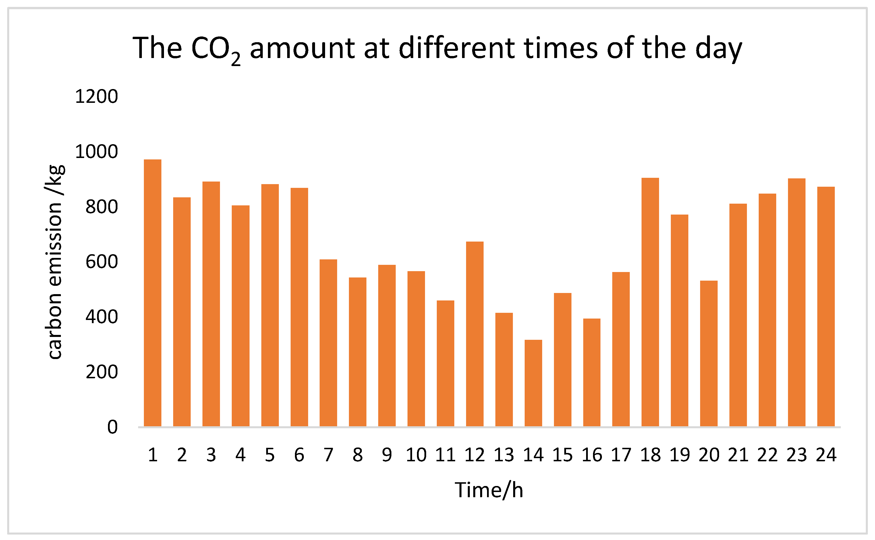
2. Indirect Carbon Emissions from Electricity and Their Uncertainty

When calculating the carbon emission cost of purchasing electricity from the external power grid in a comprehensive energy system, it is first necessary to determine the carbon emission intensity at the time period when the system is connected to the grid nodes. The carbon emission intensity calculation method for power system nodes can be referred to, and this value can be calculated based on the interaction value of the node’s electricity consumption. The formula can be expressed as follows [34]:
e G t = C k t P k t = P F , i t M F , i t C F , i t P F , i t θ F , i t + P C , j t θ C , j t
where e Grid t is the indirect carbon emission intensity of electricity at the connection node between the comprehensive energy system and the power grid during time t, tCO2/MW·h; C k t is the carbon flow from the k-th branch of time period t to this node, tCO2/s; P k t is the power flowing from the k-th branch of time period t to this node, kW; P F , i t and P C , j t , respectively, represent the electricity provided by the i-th fossil energy and j-th renewable energy flowing to this node during time period t, kW·h; M F , i t is the energy quality consumed by the i-th fossil energy source to provide a unit of electricity to the node during time period t, t; C F , i t is the carbon emissions per unit mass generated by the i-th fossil energy consumption during time period t, t; and θ F , i t and θ C , j t are the loss rates of the i-th fossil energy and the j-th renewable energy provided by the generation side to the integrated energy system and grid connection nodes during time t, respectively.
When conducting electricity scheduling, due to the volatility of wind and photovoltaic power, the sources of electricity purchased by system operators from the grid also exhibit a certain degree of randomness. According to Equation (1), the randomness of the renewable energy output P C , j t will ultimately lead to a random change in the indirect carbon emission intensity e Grid t of the grid nodes, that is, there is also uncertainty in the indirect carbon emission intensity of the integrated energy system and grid connection nodes. In this case, this uncertainty may lead to inaccurate carbon emissions of grid-connected integrated energy systems, which in turn affects the economic and environmental benefits of the system. Similar methods can be adopted to address the uncertainty of wind and solar power. Polyhedral uncertainty sets are widely used due to their linear structure and the ease of adjusting the conservatism of scheduling strategies. Therefore, in this section, polyhedral uncertainty sets are used to characterize the range of uncertain parameter values. The expression is shown in Equation (2):
U 1 = t T Δ e Grid t Δ e Grid t , max Γ G r i d e Grid t = e Grid t + Δ e Grid t
where U 1 is the uncertainty set of indirect carbon emission intensity from electricity at the connection node between the integrated energy system and the power grid; T is a scheduling cycle, usually 24 h; e Grid t is the predicted value of the indirect carbon emission intensity of the connected node’s electricity during time period t, tCO2/MW·h; Δ e Grid t represents the deviation between the predicted and actual carbon emission intensity values of time period t and the grid connection nodes, tCO2/MW·h; Δ e Grid t , max is the maximum deviation between the actual and predicted values of indirect carbon emissions intensity from electricity during time period t, tCO2/MW·h; Γ G r i d is the robustness coefficient for controlling the range of variation of the uncertain parameter.
Due to the random volatility of renewable energy sources such as wind and solar power on the power generation side, as well as the susceptibility of the load side to irregular user behavior, there is still the challenge of inaccurate predicted values. The output range of photovoltaic and wind turbines can be represented by the following equation:
U 2 = U PV , U WT , U P , U H , U C
Taking photovoltaics as an example, the uncertainty features of polyhedral uncertainty sets are characterized as follows. The characterization methods for other uncertain parameters are similar and will not be repeated here.
U P V = t T Δ P P V t Δ P P V t , max Γ P V P P V t = P P V t + Δ P P V t
where U 2 is the uncertainty set of photovoltaic, fan output, and electrical, thermal, and cooling loads; U P V , U WT , U P , U H , U C are the uncertainty sets of photovoltaic, fan, electricity, heat, and cooling loads, respectively; P P V t is the actual value of photovoltaic output during the t period of the integrated energy system, kW; P P V t is the predicted value of PV output during the t period, kW; Δ P P V t is the deviation between the actual PV output value and the predicted value during the period t, kW; Δ P P V t , max is the maximum deviation between the actual value and the predicted value of PV output during the period t, kW; and Γ P V is a robust parameter that controls the variation range of the uncertain parameter.
Carbon trading is an effective way to control carbon dioxide emissions. With the promotion of the “double carbon” goal, China has gradually opened a carbon trading market (referred to as the carbon market) that can trade carbon emission rights since 2021, and encourages all emission entities to strive to reduce carbon emissions [35]. In this market, the government allocates free initial carbon emission quotas to each entity based on their actual situation. In the development process of the emitting entities, if their actual carbon emissions exceed the initially allocated carbon emission quotas, they are required to purchase additional quotas from other entities [36]. In this paper, the baseline method is adopted to determine the initial carbon emission quota of the integrated energy system. The carbon emission sources include a gas turbine, a gas boiler and power grid purchase. The initial carbon emission quota model is shown as follows:
E t = δ P PCG t + P CV t + P buy t + δ GB H GB t
where E t is the total carbon emission quota given by the government to the integrated energy system during the t period, tCO2/MW·h; δ is the emission allocation per unit of electricity, generally 0.728 tCO2/MW·h [37]; and δ GB is the carbon emission quota of the unit heat output of the gas boiler, generally 0.367 tCO2/GJ [38].
The actual carbon emissions of the integrated energy system during the t period can be expressed by the following formula:
E IES t = γ GT P GT t + γ GB H GB t + e Grid t P buy t
where E IES t is the total actual carbon emissions of the system during the period t, t; γ GT is the carbon emission coefficient of the gas turbine, tCO2/MW·h; and γ GB is the carbon emission coefficient of the gas-fired boiler, tCO2/MW·h.
Then, the carbon trading cost of the integrated energy system in the t period can be expressed as
F C t = W C O 2 ( E I E S t E t )
where F C t is the carbon trading cost of the integrated energy system during the period t, CNY; W C O 2 is the carbon price, CNY/t.

3. Integrated Energy System Modeling

In the scheduling stage, the constraints mainly include the energy balance constraint, energy interaction constraint, and equipment operation constraint of the whole system.
(1)
IES supply and demand balance constraint of electrical load:
P W T T + P P V T + P E X T + P G T T + P E S T = P L T
(2)
IES supply–demand balance constraint of heat load:
H G B T + H H P T + H G T T + H H S T = H L T
(3)
IES supply–demand balance constraint of cooling load:
C A C T + C E C T + C C S T = C L T
(4)
IES indicated device running constraints:
E G T min E G T t E G T max H G T min H G T t H G T max G T r a t e max E G T t E G T t 1 G T r a t e max
H G B min H G B t H G B max G B r a t e max H G B t H G B t 1 G B r a t e max
H H P min H H P t H H P max H P r a t e max H H P t H H P t 1 H P r a t e max
C A C min C A C t C A C max A C r a t e max C A C t C A C t 1 A C r a t e max
C E C min C E C t C E C max E C r a t e max C E C t C E C t 1 E C r a t e max
E P V min E P V t E P V max E W T min E W T t E W T max
(5)
Interaction constraints between IES and electricity and gas networks:
P E X min P E X P E X max
where E G T max , H G B max , H H P max , C A C max , C E C max , P P V max , P W T max indicate the upper power limit of the corresponding energy device, kW; G T r a t e max , G B r a t e max , H P r a t e max , A C r a t e max , E C r a t e max indicate the upper limit of power climbing for the corresponding energy equipment, kW; and E E X max is the upper limit of the system’s interaction with the power network, kW·h.
The IES energy storage devices in this paper include batteries. The energy charging and discharging processes of these devices are similar, and they all need to comply with their own power constraints, state capacity constraints, and mutually exclusive constraints of charge and discharge states. In addition, in order to ensure the service life of energy storage equipment, it is necessary to ensure the same starting and ending capacity. The ES model is as follows:
S E S , c h a t P E S , c h a min P E S , c h a t S E S , c h a t P E S , c h a max S E S , d i s t P E S , d i s min P E S , dis   t S E S , d i s t P E S , d i s max S E S , c h a t + S E S , d i s t 1 E E S t = E E S t 1 1 σ E S + η E S , c h a P E S , c h a t P E S , d i s t / η E S , d i s Δ t E E S min E E S t + 1 E E S max E E S 0 = E E S 24
where S E S , c h a t and S E S , d i s t are the charging state and discharge state, respectively; P E S , c h a m i n , P E S , c h a m a x , P E S , d i s m i n , P E S , d i s m a x are the minimum and maximum power of charge and discharge, respectively, kW; σ E S is the self-leakage rate; and η E S , c h a and η E S , d i s are, respectively, the charge and discharge efficiency.

4. Two-Stage Robust Optimization Model and Transformation

4.1. The Standard Form of a Two-Stage Robust Optimization Model

The objective function of the integrated energy system optimization model constructed in this section includes the system operating cost and carbon trading cost, and also considers the uncertainty of the indirect carbon emission intensity of electricity, wind power, photovoltaic output, and electric heating and cooling load. The model can be expressed in min–max–min form as a two-stage three-layer optimization model. The goal of the min problem is the equipment start–stop state of each system ahead of the day, and the goal of the inner max–min problem is the minimum intra-day operation cost under the worst scenario, which is expressed by the following formula:
F I E S = min x ˙ c T y max P ˜ { W } min x ˜ Φ x , P ˜ I N ( x ˜ )
where F I E S is the total cost during the operating life of the integrated energy system, CNY; x is the day-ahead cost, CNY; x ˜ is the intra-day stage cost, CNY; and P ˜ is an uncertain variable, including indirect carbon emissions from electricity, renewable energy output, and load demand.
The model constructed above is nonlinear and non-convex with three layers, which cannot be solved directly by commercial solvers or bionic optimization algorithms. However, it is not difficult to find that the uncertain variables in the model are only related to the output decision variables of the equipment, and have nothing to do with the start and stop state of the equipment. Therefore, the above model can be divided into two stages: The first stage is the day-ahead optimization stage, which aims to determine the start–stop state of each device in the system. After optimizing the decision variables, it is brought to the intra-day optimization stage of the second stage, and the influence of the uncertain variables of intra-day optimization is considered to obtain the equipment output in the intra-day scheduling stage under the worst scenario. At this point, the IES nonlinear non-convex optimization model is transformed into a solvable two-stage three-layer robust optimization model, whose formula is
min   y c T y + max u 1 U 1 , u 2 U 2 min x T y , u 1 , u 2 b T x + u 1 T x
s . t . D x d , K x = k F x + G y h H x = u 2
where y represents the start–stop variable of the advance stage of each equipment in the integrated energy system; x represents the output variable of each equipment in the integrated energy system during the day, and x and y are column vectors. In order to facilitate matrix derivation and solution, only the variables related to carbon emissions in x in u 1 T have values, and the rest are set to 0. T(y, u1, u2) represents the feasible domain of the equipment output variable x of the intra-day stage after the equipment start and stop variable of the day-ahead stage and the uncertain variable are determined; b, c represent the column vectors of the cost coefficients during operation of the integrated energy system, respectively; D, K, F, G, H represent the constraint coefficient matrix of the pre-day and intra-day decision variables of the integrated energy system, respectively; d, k, h represent constant series vectors of corresponding constraints, respectively.

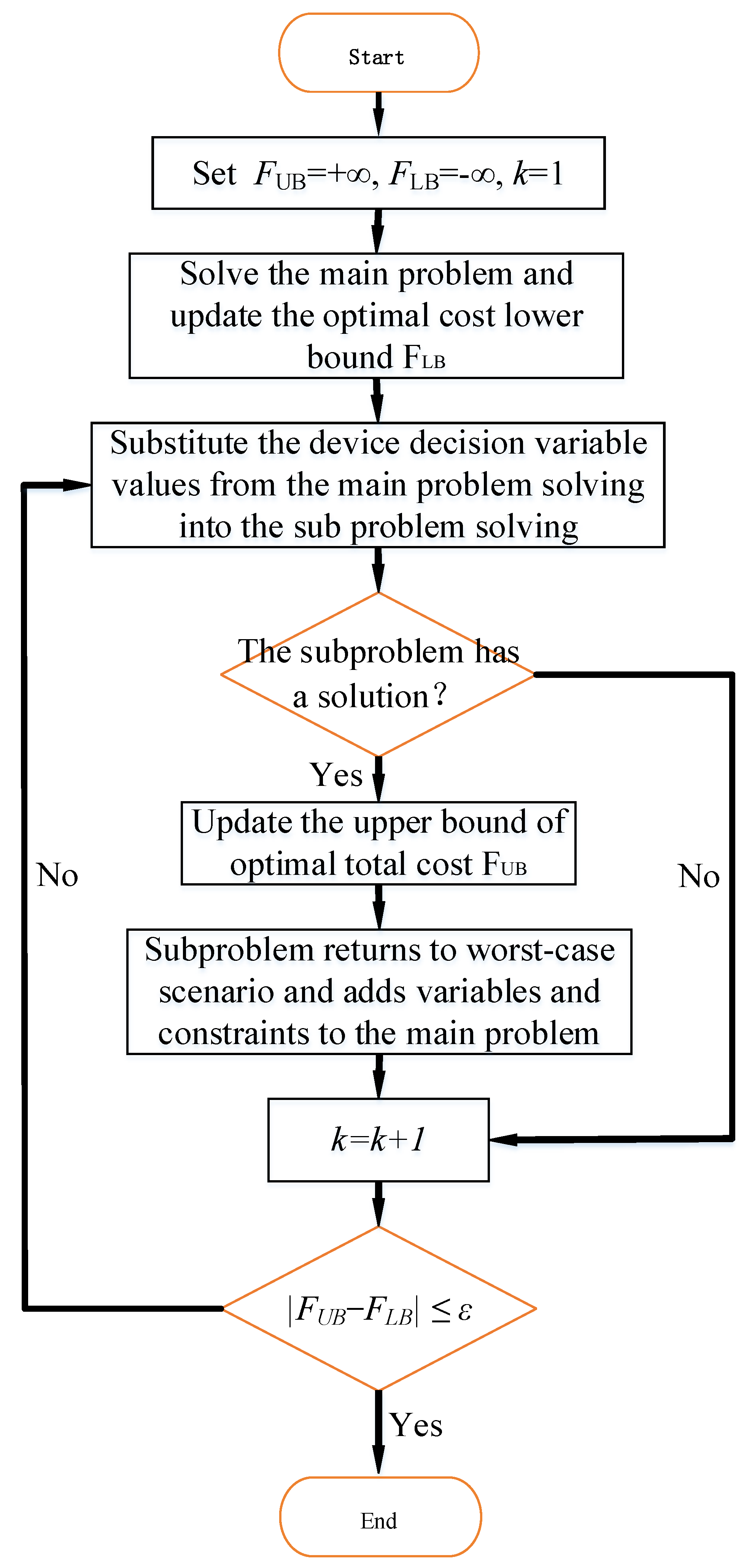
4.2. Column-and-Constraint Generation Algorithm

First, only the decision variables of the first stage and their associated constraints are considered, and this stage is regarded as a relaxed version of the whole problem. Then, the effect of the loosened part is gradually added back. In the second phase, the aim is to find the extremes. Assuming that the worst case can be directly identified, the two-stage robust optimization problem can be solved equivalently by simply returning the parameters and their constraints in this case directly to the main problem. However, it is often not feasible to fully identify all extremes. Therefore, the feasible strategy is to first set an initial value for the decision variables in the first stage, and then incorporate these initial values into the subproblems for solving. Then, the solution of the subproblem obtained at this time is the most extreme solution of the current iteration, and the decision variables and constraints in the corresponding scenario of this solution are returned to the main problem again. Through cyclic iteration, the number of worst-case scenarios considered in the main problem gradually increases, leading to a gradual improvement in the quality of the solution, and finally the optimal solution is reached. As the variables and constraints of the main problem increase, the global lower bound increases correspondingly, and the information passed from the main problem to the subproblems also changes, which helps to improve the global upper bound (i.e., lower the upper-bound value). Through this process of continuous iteration, the upper and lower bounds are continuously optimized until the algorithm converges, so the algorithm is called the column-and-constraint generation algorithm (CCG) [28].
Therefore, according to the CCG algorithm, the main problem form of the two-stage robust optimization model is
min c T y + ψ
s . t . ψ b T x l + ( u 1 l ) T x l D x l d F x l + G y h K x l = k H x l = u 2 l
where ψ represents the objective function value of the subproblem; x l is the new decision variable added from the subproblem back to the main problem for the l-th time; and u 1 l , u 2 l represent the worst-case variables that return from the subproblem to the main problem for the l-th time, respectively.
The subproblem form is as follows:
max u 1 U 1 , u 2 U 2 min x T y , u 1 , u 2 b T x + u 1 T x
s . t . D x d F x + G Y h , K x = k H x = u 2
where Y is the value of the day-ahead decision variable that has been solved for the main problem.
The algorithm flow is as follows: (1) Set the random value of the uncertain variable as the initial value, and set the lower bound of the scheduling result to negative infinity, the upper bound to positive infinity, and the initial cycle number to 1. (2) Based on the values of the uncertain parameters, solve the main problem (22) to determine the decision variable and objective function of the main problem, and set the value of the objective function as the new lower bound. (3) Substitute the decision variables obtained from the solution of the main problem into the subproblem (24) to calculate the objective function, decision variables, and updated uncertain parameter values of the subproblem. (4) Set the convergence threshold of the algorithm cycle. In this paper, 0.02 is taken to cycle the algorithm so that the upper and lower bounds of the final objective function of the system are iteratively updated until the relative difference in the values of the upper and lower bounds meets the convergence conditions, at which time the solution is completed.
The specific expression is
F L B = c T y k * + ψ k * F U B = max F U B , b T x k * + ( u 1 k * ) T x k *
where F U B , F L B represent the upper and lower bounds of the final objective function of the system, respectively, y k * , ψ k * are the decision variable values of the main problem obtained at the k-th cycle, x k * represents the value of the decision variable in the subproblem resulting from the k-th loop, and u 1 k * is the worst case obtained by solving the subproblem for the k-th time.
The specific process of CCG algorithm can be illustrated in Figure 1. The specific process of the CCG algorithm is as follows:
  • Initialization: First, set the initial state, including the initial values of the decision variables and other necessary parameters.
  • Generating candidate solutions: Based on the problem’s constraints, generate candidate solutions that satisfy the constraints, typically achieved using the Lagrange multiplier method.
  • Column generation: Select the solution from the generated candidate solutions that contributes the most to the objective function, and add it to the main problem.
  • Re-solving the main problem: Incorporate the newly added candidate solution into the main problem, and then re-solve to obtain a new optimal solution.
  • Checking stop conditions: Check whether the stop conditions are met. If they are met, stop the algorithm and output the final optimal solution. If they are not met, return to step 2 and continue generating candidate solutions.

4.3. Karush–Kuhn–Tucker Condition and Its Transformation

In the above model, the main problem of the first stage is the MILP problem, which can be solved directly by minimizing the objective function. However, the second-stage subproblem is a two-layer programming problem, which is still a nonlinear and non-convex model and cannot be solved directly, and it is easy to fall into the local optimal solution if the bionic optimization algorithm is adopted. The most commonly used methods for this model are the dual transformation and the Karush–Kuhn–Tucker condition. Due to the multiplication of bilinear variables in the objective function, the dual transformation method is difficult to transform, while the KKT condition can introduce Lagrange factors to transform the equality constraints. It is also generalized to more general inequality constraints, so as to transform an optimization model with an objective function into a model without objective function, that is, transform the minimum problem of the inner layer into the constraint conditions, and thus, the original two-layer maximum–minimum problem is transformed into a single-layer maximum problem. The specific model of the subproblem transformed by KKT conditions is as follows:
max u 1 U 1 , u 2 U 2 b T x + u 1 T x
s . t . D x d , K x = k F x + G y h H x = u 2 λ 1 , λ 2 0 λ 1 ( d D x ) = 0 λ 2 ( F x G y ) = 0 b + u 1 D T λ 1 F T λ 2 + G T ω 1 + H T ω 2 = 0
where λ 1 , λ 2 , respectively, represent the auxiliary variables introduced in the derivation transformation of inequality constraints using KKT conditions; ω 1 , ω 2 , respectively, represent the auxiliary variables introduced in the derivation transformation of equality constraints using KKT conditions; constraint lines 5 to 7 represent the relaxation constraints introduced when KKT conditions are used; and lines 8 to 9 represent the first-order differential equations obtained when Lagrange functions are constructed using KKT conditions. For bilinear variables in this model, the McCormick envelope method can be used for relaxation processing to simplify the model and speed up the solution. See Appendix A for the steps.
In addition, when the subproblem has a solution, all the uncertain parameters above will take the constrained boundary values, so taking the PV uncertainty set as an example, it can be converted into the following form:
U 2 = t T ( k P V , 1 t + k P V , 2 t ) Γ P V P P V t = P P V t + k P V , 1 t Δ P P V t , max k P V , 1 t Δ P P V t , max 0 k P V , 1 t + k P V , 2 t 1
where k P V , 1 t and k P V , 2 t are 0–1 variables introduced into the conversion of the PV uncertainty set, respectively. When k P V , 1 t is 1, it means that the photovoltaic output value in the t period reaches the maximum value of its change range, and when k P V , 2 t is 1, it means that the photovoltaic output value in the t period reaches the minimum value of its change interval.

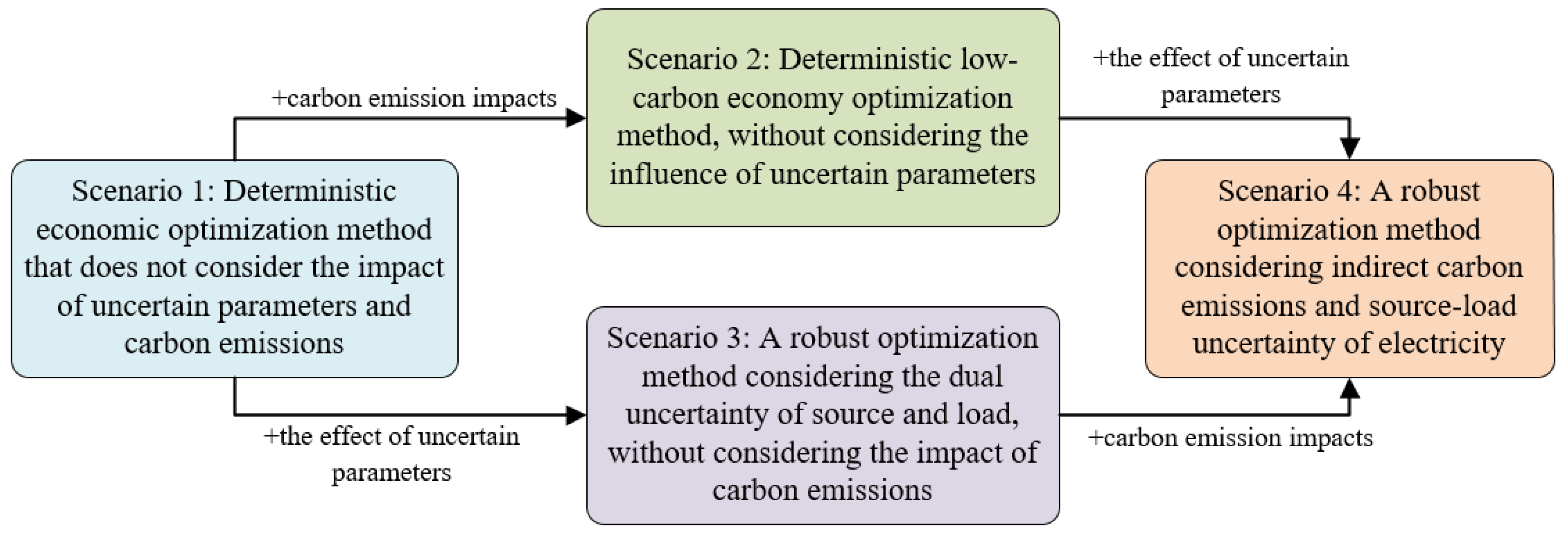
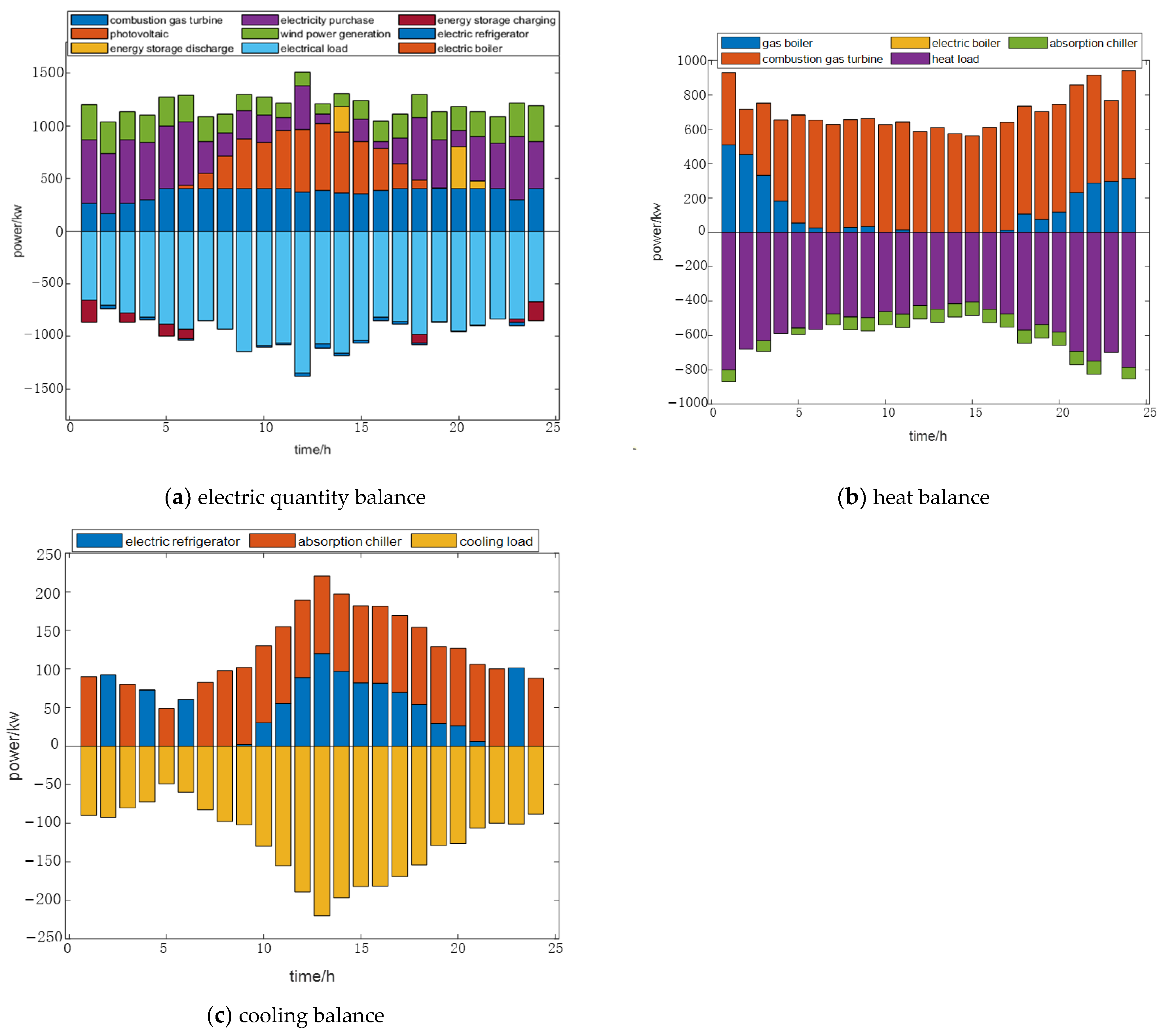
5. The Application of the Algorithm

In this section, a typical integrated energy system of a certain park is also selected as a case study for analysis, and its structure is shown in Figure 2 to verify the improvement in the system economy and low-carbon performance of the strategy proposed in this section. The purchase price of electricity from the grid is shown in Table 1, and the time-sharing price is also adopted. The predicted and actual values of PV fan output, power indirect carbon emission intensity, power, heat, cooling load, and power indirect carbon emission intensity are shown in the scheduling result diagram below, and the robust regulation coefficient Γ of the above uncertain parameters is taken as 10 in this paper. Table 2 is the parameters of energy storage equipment, Table 3 is the parameters of other equipment. The equipment parameters of the integrated energy system in this section are the same as those in Section 4 and will not be introduced here. In addition, the carbon emission price adopted in this section is the global average carbon emission price of 250 CNY/t in 2024. Table 1 shows the time-of-use electricity price of this study based on the electricity price of the Hebei Power grid [39]. Since the calculation of carbon emission intensity of power system nodes is not the focus of this paper, it will not be shown here and will be carried out in detail in the next stage. This example simulation was carried out on a computer configured with an Intel Core i7-8700 3.20 GHz processor and 16 GB memory. Matlab R2019b was used as the programming environment, the Yalmip 0.9.7 toolbox was used for modeling, and the Gurobi version 10.0 commercial solver was used for solving.
In order to verify the effect of the proposed method on the disturbance resistance of the integrated energy system, four scenarios are set for comparison, and the actual total operating costs and carbon emissions of the integrated energy system under different scenarios are analyzed. Scenario 1 adopts the deterministic economic optimization method without considering the influence of uncertain parameters and carbon emission. The second scenario is to adopt the deterministic low-carbon economy optimization method without considering the influence of uncertain parameters. Scenario 3 is a robust optimization method considering only source-load double uncertainty. Scenario 4 is a robust optimization method considering indirect carbon emissions and source-load uncertainties. Figure 3 is a diagram of the relationship between the four scenarios. The total cost, equipment operation cost, carbon emission cost, and carbon emissions of the integrated energy system obtained by solving the four scenarios are shown in Table 4. Figure 4 shows the amount of carbon dioxide emitted at different times of the day. It can be seen that the carbon emission is higher at 0–6 h and 21–24 h of the day. At this time, the system heat load is higher and the gas boiler output is higher, leading to higher system carbon emissions.
As can be seen from the above Table 4, the total cost of scenario 1 is the lowest after the system optimization calculation. This is because this method is the simplest deterministic optimization method and does not consider the impact of uncertainty and carbon emission, resulting in a very ideal result and high carbon emission. In practical engineering, operators do not apply this scheduling strategy because of poor anti-fluctuation interference. In scenario 2, after the introduction of the carbon trading mechanism, although the carbon emissions are reduced by 2.57%, the cost is increased by 11.6%, and the deterministic optimization method is also adopted, resulting in unavailable scheduling results. The cost of scenario 3 increases after considering the influence of uncertainty. This is because the optimization method considers the worst scenario and needs an increase in cost to compensate for the scheduling result, which has better practical application value than scenario 1. On the basis of scenario 3, scenario 4 also considers the uncertainty of indirect carbon emissions of electricity. Both optimization methods can enhance the ability of the system to resist fluctuation risks. However, compared with scenario 3 which only considers the uncertainty of source-load, the strategy proposed in scenario 4 still reduces the total cost by 5.03% and carbon emissions by 1.25%, which is because the carbon emission calculation by this method is more accurate. The system can have excess carbon emission rights that can be traded to earn revenue, reducing operating costs and carbon emissions.
According to the method presented above, the optimization results of scenario 4 are shown in Figure 5 and Figure 6. It can be seen that due to the lack of photovoltaic power during the 1–6 period, the output of renewable energy is only wind turbines. At this time, it is in the valley electricity price stage, and purchasing electricity from the grid is more economical than gas turbine power generation. Most of the electricity is supplemented by purchasing electricity from the grid, and wind turbines can supply a portion of the electricity. The excess can be charged to the battery. All cooling loads are supplied by electric refrigeration units. For heat load, it is mainly supplied by gas boilers and gas turbines. Starting from 5 o’clock, the heating output of gas turbines gradually increases, and from 6 o’clock to 24 o’clock, it is mainly supplied by gas turbines with auxiliary heating from gas boilers. At 7–10 o’clock, the heat load of the system is lower and the cold load is higher due to a slight increase in electricity prices and the gradual increase in electricity from photovoltaics; it is not economical to purchase electricity from the grid at this time, and the cost of gas turbines is relatively low. Therefore, when the system starts the gas turbine to produce electricity, the waste heat can be used as the main source of heat load supply, while the gas boiler serves as a supplement to meet the remaining demand for heat load. For cooling load, electric refrigeration is the main supply method, while absorption refrigeration provides an additional cooling capacity when necessary. At 8 o’clock, due to insufficient power supply, all cooling loads were supplied by absorption refrigeration units. In addition, starting from 18:00, the photovoltaic system stops outputting, and the wind and gas turbines reach their output limits. At this time, the battery can release some supplementary electricity to achieve peak shaving and valley filling.

6. Summary

This study systematically introduces the theory of uncertainty optimization and explores robust interval optimization as a more risk-resistant method.
Firstly, regarding the theory of uncertainty sets, a detailed comparative analysis was conducted on three commonly used uncertainty sets, and it was determined to use polyhedral uncertainty sets to describe the introduction of three uncertain variables: wind turbines, photovoltaics, and indirect carbon emissions from electricity.
Secondly, a two-stage three-layer robust low-carbon economic optimization scheduling model for integrated energy systems was constructed, and the column-and-constraint generation algorithm was used to transform it into a single-layer main problem and a two-layer sub problem for iterative solution. The dual layer subproblem was transformed into a linear programming model using the Karush–Kuhn–Tucker condition, and solved to obtain the system’s operating results and scheduling scheme.
Finally, through case analysis, it was found that although introducing uncertainty optimization would increase system costs and carbon emissions, the proposed scheduling strategy has stronger stability and significantly reduces the impact of uncertain factors on the system. Compared to only considering the source load uncertainty scenario, the method proposed in this paper can reduce the total system cost by 5.03% and carbon emissions by 1.25%, thus verifying the effectiveness and practicality of the proposed method.

Author Contributions

N.L.: Conceptualization; methodology; software; writing—original draft; writing—review and editing. B.Z.: Software; writing—original draft. G.W.: Software; writing—original draft. W.L.: Methodology; software. D.G.: Writing—review and editing. L.Z.: Methodology; software. C.P.: Writing—review and editing. All authors have read and agreed to the published version of the manuscript.

Funding

This paper is supported by the State Grid Comprehensive Energy Service Group Co., Ltd. Technology Project “Research on Carbon Emission Management Standard System and Key Technical Standards for Comprehensive Energy Services”, project No. 527899220006.

Data Availability Statement

The original contributions presented in the study are included in the article, further inquiries can be directed to the corresponding author.

Conflicts of Interest

Authors Na Li, and Dongxu Guo were employed by the company State Grid Integrated Energy Services Group Co., Ltd. The remaining authors declare that the research was conducted in the absence of any commercial or financial relationships that could be construed as a potential conflict of interest. The company had no role in the design of the study; in the collection, analyses, or interpretation of data; in the writing of the manuscript, or in the decision to publish the results.

Nomenclature

C F , i t The carbon emissions generated per unit mass of the i-th type of fossil energy consumption, t
C k t The carbon flow of the k-th branch towards this node, tCO2/s
E t The government provides the system with a total carbon emission quota for time period t, tCO2/MW·h
E I E S t The total actual carbon emissions of the system during time period t, t
E G T max Power upper limit of energy equipment, kW
E E X max The upper limit of interaction between the system and the power network, kW·h
e Grid t Indirect carbon emission intensity of electricity
e Grid t Predictive value of indirect carbon emission intensity from electricity, tCO2/MW·h
F C t The carbon trading cost of the system during time period t, CNY
F I E S The total cost during the system operation cycle, CNY
G T r a t e max Upper limit of power ramp-up for energy equipment, kW
M F , i t The energy quality consumed per unit of electricity provided by the i-th type of fossil energy to the node, t
P k t The power flowing from the k-th branch to this node, kW
P F , i t The electricity provided by the i-th type of fossil energy flowing to this node, kW·h
P P V t Actual value of photovoltaic output during period t of the system, kW
P P V t Predictive value of photovoltaic output during system t period, kW
P E S , c h a m i n Minimum charging power, kW
P ˜ Uncertainty variable capture equipment, kW
S E S , c h a t The charging status of the battery
S E S , d i s t The discharge state of the battery
x ˜ Daily stage cost, CNY
x Current cost, CNY
Γ G r i d Robust coefficient for controlling the range of uncertain parameter changes
η E S Battery charging and discharging efficiency
θ F , i t The loss rate of electricity transmission provided by the i-th type of fossil energy
σ E S Self-leakage rate

Appendix A. McCormick Envelope Method

The McCormick envelope method is suitable for convex relaxation of non-convex programming models that multiply bilinear variables, that is, transforming a nonlinear non-convex programming model into a nonlinear convex programming model through constraint relaxation. In addition, the McCormick envelope method is a special relaxation method that not only maintains the convexity of the model, but also provides the boundary closest to the original solution.
Assuming a general non-convex function, the McCormick envelope method can be used to relax the function into a convex function. Then, this new problem can be solved as a nonlinear programming problem, which will generate a lower bound solution to the original problem, and thus the original problem can converge. For example:
Z = min i j c i j x i x j + g o x
s . t . i j c l i j x i x j + g l x 0 l L
x L x x U
By replacing x i x j = w i j , the above non-convex programming model can be transformed into the following convex programming model:
Z = min i j c i j w i j + g o x
w i j x i L x j + x i x j L x i L x j L w i j x i U x j + x i x j U x i U x j U w i j x i U x j + x i x j L x i U x j L w i j x i x j U + x i L x j x i L x j U x L x x U w L w w U
If g(x) is a linear function, then the original model becomes a linear programming model that can converge to the minimum solution of the original model, and vice versa.

References

  1. Feng, C.; Liao, X. An overview of “Energy + Internet” in China. J. Clean. Prod. 2020, 258, 120630. [Google Scholar] [CrossRef]
  2. Hannan, M.A.; Ker, P.J.; Mansor, M.; Lipu, M.H.; Al-Shetwi, A.Q.; Alghamdi, S.M.; Begum, R.A.; Tiong, S.K. Recent advancement of energy internet for emerging energy management technologies: Key features, potential applications, methods and open issues. Energy Rep. 2023, 10, 3970–3992. [Google Scholar] [CrossRef]
  3. Chang, P.; Li, C.; Zhu, Q.; Zhu, T.; Shi, J. Optimal scheduling of electricity and hydrogen integrated energy system considering multiple uncertainties. iScience 2024, 27, 109654. [Google Scholar] [CrossRef] [PubMed]
  4. Martinez-Mares, A.; Fuerte-Esquivel, C.R. A Robust Optimization Approach for the Interdependency Analysis of Integrated Energy Systems Considering Wind Power Uncertainty. IEEE Trans. Power Syst. 2013, 28, 3964–3976. [Google Scholar] [CrossRef]
  5. Mei, F.; Zhang, J.; Lu, J.; Lu, J.; Jiang, Y.; Gu, J.; Yu, K.; Gan, L. Stochastic optimal operation model for a distributed integrated energy system based on multiple-scenario simulations. Energy 2021, 219, 119629. [Google Scholar] [CrossRef]
  6. Lin, S.; Liu, C.; Shen, Y.; Li, F.; Li, D.; Fu, Y. Stochastic Planning of Integrated Energy System via Frank-Copula Function and Scenario Reduction. IEEE Trans. Smart Grid 2022, 13, 202–212. [Google Scholar] [CrossRef]
  7. Wu, M.; Yan, R.; Zhang, J.; Fan, J.; Wang, J.; Bai, Z.; He, Y.; Cao, G.; Hu, K. An enhanced stochastic optimization for more flexibility on integrated energy system with flexible loads and a high penetration level of renewables. Renew. Energy 2024, 227, 120502. [Google Scholar] [CrossRef]
  8. Yan, Y.; Huang, C.; Guan, J.; Zhang, Q.; Cai, Y.; Wang, W. Stochastic optimization of solar-based distributed energy system: An error-based scenario with a day-ahead and real-time dynamic scheduling approach. Appl. Energy 2024, 363, 123099. [Google Scholar] [CrossRef]
  9. Dong, B.; Li, P.; Yu, H.; Ji, H.; Song, G.; Li, J.; Zhao, J.; Wang, C. Chance-constrained optimal dispatch of integrated energy systems based on data-driven sparse polynomial chaos expansion. Sustain. Energy Technol. Assess. 2023, 60, 103546. [Google Scholar] [CrossRef]
  10. Wang, C.; Ju, P.; Wu, F.; Lei, S.; Pan, X. Long-Term Voltage Stability-Constrained Coordinated Scheduling for Gas and Power Grids with Uncertain Wind Power. IEEE Trans. Sustain. Energy 2022, 13, 363–377. [Google Scholar] [CrossRef]
  11. Aguilar, J.; Bordons, C.; Arce, A. Chance Constraints and Machine Learning integration for uncertainty management in Virtual Power Plants operating in simultaneous energy markets. Int. J. Electr. Power Energy Syst. 2021, 133, 107304. [Google Scholar] [CrossRef]
  12. Wu, G.; Li, T.; Xu, W.; Xiang, Y.; Su, Y.; Liu, J.; Liu, F. Chance-constrained energy-reserve co-optimization scheduling of wind-photovoltaic-hydrogen integrated energy systems. Int. J. Hydrogen Energy 2023, 48, 6892–6905. [Google Scholar] [CrossRef]
  13. Fan, H.; Wang, C.; Liu, L.; Li, X. Review of Uncertainty Modeling for Optimal Operation of Integrated Energy System. Front. Energy Res. 2022, 9, 641337. [Google Scholar] [CrossRef]
  14. Li, X.; Zhang, L.; Wang, R.; Sun, B.; Xie, W. Two-Stage Robust Optimization Model for Capacity Configuration of Biogas-Solar-Wind Integrated Energy System. IEEE Trans. Ind. Appl. 2023, 59, 662–675. [Google Scholar] [CrossRef]
  15. Silva-Rodriguez, L.; Sanjab, A.; Fumagalli, E.; Gibescu, M. Light robust co-optimization of energy and reserves in the day-ahead electricity market. Appl. Energy 2024, 353, 121982. [Google Scholar] [CrossRef]
  16. Gao, J.; Yang, Y.; Gao, F.; Wu, H. Two-Stage Robust Economic Dispatch of Regional Integrated Energy System Considering Source-Load Uncertainty Based on Carbon Neutral Vision. Energies 2022, 15, 1596. [Google Scholar] [CrossRef]
  17. Jiang, R.; Wang, J.; Guan, Y. Robust Unit Commitment with Wind Power and Pumped Storage Hydro. IEEE Trans. Power Syst. 2012, 27, 800–810. [Google Scholar] [CrossRef]
  18. Wang, P.; Zheng, L.; Diao, T.; Huang, S.; Bai, X. Robust Bilevel Optimal Dispatch of Park Integrated Energy System Considering Renewable Energy Uncertainty. Energies 2023, 16, 7302. [Google Scholar] [CrossRef]
  19. Zong, X.; Yuan, Y. Two-stage robust optimization of regional integrated energy systems considering uncertainties of distributed energy stations. Front. Energy Res. 2023, 11, 1135056. [Google Scholar]
  20. Zhao, Y.; Wei, Y.; Zhang, S.; Guo, Y.; Sun, H. Multi-Objective Robust Optimization of Integrated Energy System with Hydrogen Energy Storage. Energies 2024, 17, 1132. [Google Scholar] [CrossRef]
  21. Zhou, C.; Jia, H.; Jin, X.; Mu, Y.; Yu, X.; Xu, X.; Li, B.; Sun, W. Two-stage robust optimization for space heating loads of buildings in integrated community energy systems. Appl. Energy 2023, 331, 120451. [Google Scholar] [CrossRef]
  22. Zhang, Y.; Zheng, F.; Shu, S.; Le, J.; Zhu, S. Distributionally robust optimization scheduling of electricity and natural gas integrated energy system considering confidence bands for probability density functions. Int. J. Electr. Power Energy Syst. 2020, 123, 106321. [Google Scholar] [CrossRef]
  23. Wang, M.; Shi, Z.; Luo, W.; Sui, Y.; Wu, D. Distributionally robust optimal scheduling of integrated energy systems including hydrogen fuel cells considering uncertainties. Energy Rep. 2023, 10, 1575–1588. [Google Scholar] [CrossRef]
  24. Cai, P.; Mi, Y.; Ma, S.; Li, H.; Li, D.; Wang, P. Hierarchical game for integrated energy system and electricity-hydrogen hybrid charging station under distributionally robust optimization. Energy 2023, 283, 128471. [Google Scholar] [CrossRef]
  25. Zhou, D.; Zhu, Z. Urban integrated energy system stochastic robust optimization scheduling under multiple uncertainties. Energy Rep. 2023, 9, 1357–1366. [Google Scholar] [CrossRef]
  26. Zhang, G.; Wen, J.; Xie, T.; Zhang, K.; Jia, R. Bi-layer economic scheduling for integrated energy system based on source-load coordinated carbon reduction. Energy 2023, 280, 128236. [Google Scholar]
  27. Li, F.; Wang, D.; Guo, H.; Zhang, J. Distributionally Robust Optimization for integrated energy system accounting for refinement utilization of hydrogen and ladder-type carbon trading mechanism. Appl. Energy 2024, 367, 123391. [Google Scholar] [CrossRef]
  28. Yang, B.; Ge, S.; Liu, H.; Zhang, X.; Xu, Z.; Wang, S.; Huang, X. Regional integrated energy system reliability and low carbon joint planning considering multiple uncertainties. Sustain. Energy Grids Netw. 2023, 35, 101123. [Google Scholar]
  29. Shi, Z.; Yang, Y.; Xu, Q.; Wu, C.; Hua, K. A low-carbon economic dispatch for integrated energy systems with CCUS considering multi-time-scale allocation of carbon allowance. Appl. Energy 2023, 351, 121841. [Google Scholar] [CrossRef]
  30. Wu, Q.; Li, C. Economy-environment-energy benefit analysis for green hydrogen based integrated energy system operation under carbon trading with a robust optimization model. J. Energy Storage 2022, 55, 105560. [Google Scholar]
  31. Zhou, Y.; Ge, J.; Li, X.; Zang, H.; Chen, S.; Sun, G.; Wei, Z. Bi-level distributionally robust optimization model for low-carbon planning of integrated electricity and heat systems. Energy 2024, 302, 131777. [Google Scholar] [CrossRef]
  32. Yang, D.; Xu, Y.; Liu, X.; Jiang, C.; Nie, F.; Ran, Z. Economic-emission dispatch problem in integrated electricity and heat system considering multi-energy demand response and carbon capture Technologies. Energy 2022, 253, 124153. [Google Scholar] [CrossRef]
  33. Yang, W.; Huang, Y.; Zhang, T.; Zhao, D. Mechanism and analytical methods for carbon emission-exergy flow distribution in heat-electricity integrated energy system. Appl. Energy 2023, 352, 121980. [Google Scholar] [CrossRef]
  34. Ding, N.; Guo, P.; Xi, Y.; Zhang, A.; Lei, X. Low-carbon development in power systems based on carbon emission analysis models: A comprehensive review. Sustain. Energy Technol. Assess. 2024, 65, 103774. [Google Scholar] [CrossRef]
  35. Zhang, J.; Liu, Z. Low carbon economic scheduling model for a park integrated energy system considering integrated demand response, ladder-type carbon trading and fine utilization of hydrogen. Energy 2024, 290, 130311. [Google Scholar] [CrossRef]
  36. Shen, H.; Zhang, H.; Xu, Y.; Chen, H.; Zhang, Z.; Li, W.; Su, X.; Xu, Y.; Zhu, Y. Two stage robust economic dispatching of microgrid considering uncertainty of wind, solar and electricity load along with carbon emission predicted by neural network model. Energy 2024, 300, 131571. [Google Scholar] [CrossRef]
  37. Zhou, X.; Cai, C.; Li, Y.; Wu, J.; Zhan, Y.; Sun, Y. A robust optimization model for demand response management with source-grid-load collaboration to consume wind-power. Glob. Energy Interconnect. 2023, 6, 738–750. [Google Scholar] [CrossRef]
  38. Zhang, B.; Xia, Y.; Peng, X. Robust optimal dispatch strategy of integrated energy system considering CHP-P2G-CCS. Glob. Energy Interconnect. 2024, 7, 14–24. [Google Scholar] [CrossRef]
  39. Hebei Development and Reform Commission. 6 December 2022. Available online: https://hbdrc.hebei.gov.cn/zcfg_1238/szcfg/202309/t20230906_86169.html (accessed on 6 December 2022).
Figure 1. CCG algorithm flow chart.
Processes 12 01921 g001
Figure 2. Integrated energy system structure diagram.
Processes 12 01921 g002
Figure 3. Diagram of the relationship between the four scenarios.
Processes 12 01921 g003
Figure 4. The CO2 amount at different times of the day.
Processes 12 01921 g004
Figure 5. Comparison of the actual values with the predicted values.
Processes 12 01921 g005
Figure 6. Scenario 4 optimization results.
Processes 12 01921 g006
Table 1. Electricity price parameters.
TypeTimePurchasing Price (CNY/(kW·h)
Peak hour11:00–15:00, 19:00–21:001
Normal period8:00–10:00, 16:00–18:00, 22:00–24:000.55
Valley period1:00–7:000.2
Table 2. Parameters of energy storage equipment.
EquipmentSELF-Attrition RateCharge/Discharge EfficiencyMinimumMaximumOriginal StateMaximum Charge and Discharge RateMaintenance Cost/(CNY·kW−1)
accumulator0.010.950.20.80.30.20.0018
Table 3. Other equipment technical parameters.
EquipmentRated EfficiencyCapacityMaintenance Cost/(CNY·kW−1)
GT0.32/0.544000.025
GB0.96000.04
EB0.942000.01
AC1.31000.012
EC31200.012
Table 4. Comparison of the results of each scene.
ScenarioTotal Cost/CNYRunning Cost/CNYCarbon Emission Cost/CNYCarbon Emission/kg
17556.667556.66012,884.99
28438.967563.86875.1012,553.23
312,205.6012,205.60016,872.14
411,590.9812,148.19−557.2116,661.94
Disclaimer/Publisher’s Note: The statements, opinions and data contained in all publications are solely those of the individual author(s) and contributor(s) and not of MDPI and/or the editor(s). MDPI and/or the editor(s) disclaim responsibility for any injury to people or property resulting from any ideas, methods, instructions or products referred to in the content.

