The Influence of Pre-Lift Gate Opening on the Internal and External Flow Characteristics During the Startup Process of an Axial Flow Pump

Abstract

This paper focuses on a vertical axial flow pump and employs a 1D-3D coupling method to investigate the effects of different gate pre-opening angles on the internal and external flow characteristics of the axial flow pump during startup. Through comparative analysis, the following conclusions are drawn: In the study, a fully open gate is defined as 1, while a fully closed gate is defined as 0. When starting the axial flow pump with different valve pre-opening degrees, backflow occurs within the first 20 s of startup, and the backflow rate inside the pump gradually increases with the increase in the valve pre-opening degree. At a valve pre-opening degree of 0.6, the maximum backflow rate inside the pump reaches 5.89% of the rated flow rate. When starting the pump with the valve fully open, the maximum backflow rate reaches 10.98% of the rated flow rate, and the efficiency is affected by the backflow rate. The valve pre-opening degree has little impact on the axial force acting on the impeller during startup. When starting with a valve pre-opening degree of 0.6, the internal pressure difference in the pump is minimized. Within the first 20 s of startup, the internal pressure difference in the impeller is 28.96% higher and the flow velocity is 14.62% higher with valve pre-opening degrees of 0.8 and 1.0 compared to a 0.6 degree opening. During the initial stage of pump startup, with valve pre-opening degrees of 0.8 and 1.0, the pressure fluctuation amplitude inside the pump is minimal, with maximum relative amplitudes of only 0.621 and 0.525, which are 41.00% and 28.51% lower than the maximum amplitudes at 0 and 0.2 degrees, respectively. In summary, the peak pressure inside the pump is minimized when the valve pre-opening degree is around 0.8, while the pressure difference and flow velocity are relatively lower at a pre-opening degree of 0.6. It is recommended to start the pump with a valve pre-opening degree of around 0.6 to 0.8.

1. Introduction

In large pump stations in our country, the types of pumps used include axial flow, mixed flow, through-flow, and centrifugal pumps, among which vertical axial flow pumps are the most commonly used. Vertical axial flow pumps feature a small footprint, low head, high flow rate, stable operation, and ease of installation and maintenance [1]. They are widely used in various fields such as flood control and drainage, agricultural irrigation, field drainage, and inter-regional water transfer [2], playing a significant role in the national economy and development. During the startup transient process of an axial flow pump, the transient characteristics such as the pump speed, head, and flow rate vary significantly [3]. The method of pump startup has a crucial impact on the system’s safety, stability, and efficiency. Different pump startup methods exhibit distinct characteristics in terms of dynamic performance, energy consumption, and structural stress. In-depth study of the characteristics and effects of various startup methods helps to optimize the pump startup process, reduce impacts on the pump and piping system, extend the equipment lifespan, and improve system operational efficiency.

Currently, research on the startup process of axial flow pumps mainly employs one-dimensional calculation methods [4]. By applying reasonable simplifications and approximations, the water flow is approximated as a one-dimensional flow, and then an appropriate mathematical model is introduced for solving and analysis [5]. Zhang et al. [6] provided the time-frequency patterns of fluid pressure fluctuations and structural vibrations at the same location in vertical axial flow pumps, offering important theoretical guidance for the optimization design and safe operation of vertical axial flow pumps. Guo et al. [7] found that due to the end wall effect, there is a significant discrepancy between the calculated and design values of the flow field structure. When designing axial flow pumps, the impact of the crowding factor should be considered. Zhang et al. [8] discovered that a pump device equipped with a pre-opened vacuum relief valve experiences significantly reduced influence from transient impact characteristics on its flow field during the pump startup process. Currently, for many large-scale units, a 1D-3D coupling approach is mostly used for calculations. Song [9] employed a 1D-3D coupling numerical simulation method to perform the numerical simulation and analysis of a typical transient process at a pumped storage power station. Liu [10] used a 1D-3D software coupling calculation method to study the intake and exhaust systems of the TBD620V12 diesel engine under real operating conditions. Fu et al. [11] developed a one-dimensional and three-dimensional (1D-3D) coupled transient flow simulation method to study the effects of nonlinear fluctuations in pressure and hydraulic thrust on the impeller. Wang [12] conducted a comparative analysis using both one-dimensional simulation and 1D-3D coupled simulation methods to study the impact of the geometric structure of the airflow transmission pipeline on the performance of a five-stroke engine. Liu et al. [13] used a one-dimensional and three-dimensional (1D-3D) coupled computational fluid dynamics (CFD) method to simulate the extreme scenario of two pump-turbines simultaneously suppressing the load in a prototype of a pumped storage system. Liu et al. [14] employed a one-dimensional and three-dimensional coupled computational fluid dynamics method to simulate the 100% load rejection transient process of a medium-head power plant. They analyzed the evolution and impact of cavitation cavities and evaluated the safety implications. Lv et al. [15], based on a 1D-3D coupling method and dynamic mesh technology, simulated the process of guide vane closure during pump shutdown for an ultra-high-head pumped storage unit. Tang et al. [16] used a one-dimensional and three-dimensional (1D-3D) coupled method along with a fluid–structure interaction (FSI) method to simulate the evolution of rotational dynamic stress in a prototype pump-turbine during the load suppression transient process. The above studies indicate that 1D-3D coupling is widely used across various fields. This method simplifies the computation process by using three-dimensional simulation for the parts that require detailed analysis and one-dimensional simulation for other parts, facilitating the exploration of internal flow characteristics.

In studies on the flow characteristics during pump startup, Cheng et al. [17] found that during the start-up of a centrifugal pump, increasing the valve opening caused a time lag for the flow to reach a steady state. Zhang et al. [18] investigated the effects of flap valves of different sizes on synchronous and asynchronous startup and shutdown processes in large axial flow pump systems. Zheng et al. [19] analyzed the flow dynamics of jet pumps under different valve openings using the velocity triangle method. Zhang et al. [8] conducted numerical simulations of the startup process of axial flow pump stations under two modes: pre-opening the vacuum breaker valve and keeping the vacuum breaker valve closed. To improve the safety and stability of pumps during startup, Xuan et al. [20] proposed a new segmented startup strategy and conducted experimental studies on the stability of mixed flow pumps during segmented startup. From the above descriptions, it is evident that research on pump startup processes has predominantly focused on mixed flow and centrifugal pumps, with limited studies on the valve opening methods during the startup of vertical axial flow pumps. Therefore, to investigate the internal and external characteristics of vertical axial flow pumps during startup with different gate pre-opening degrees, this paper employs a combination of one-dimensional calculations and one-three-dimensional coupling to perform numerical simulations of the flow conditions when the axial flow pump unit is started with different gate pre-opening degrees. This study further optimizes the startup process of axial flow pumps, improving the efficiency and stability of the pump during startup.

2. Model and Methods

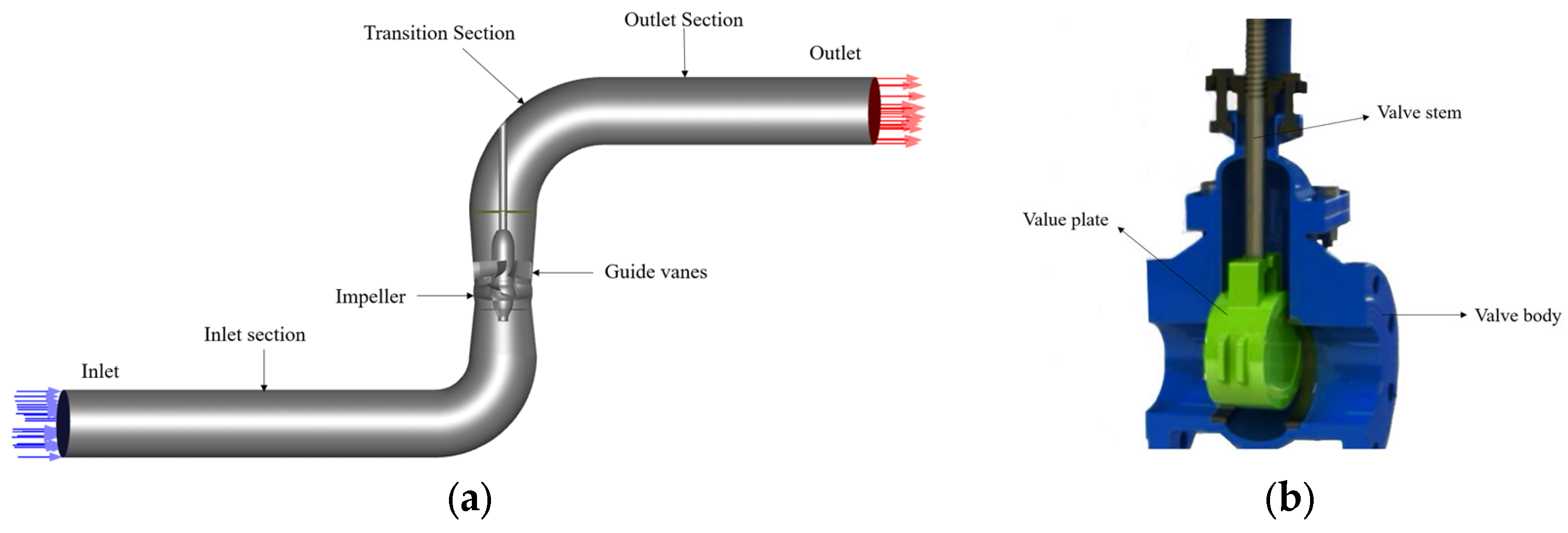
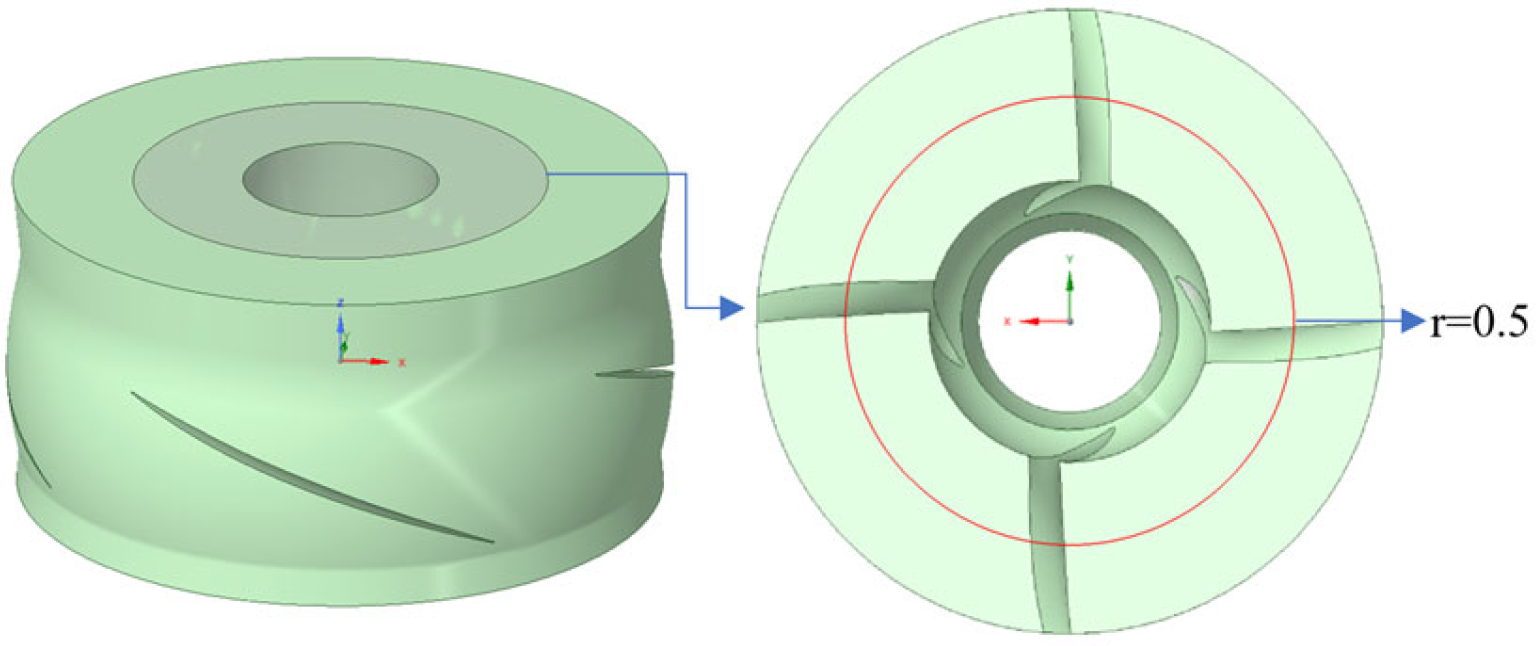
2.1. Model Parameters

The Cero 8.0 software was used to model the three-dimensional fluid domain of the vertical axial flow pump. The model includes four parts: the intake section, impeller, guide vanes, and discharge section. The design flow rate of the pump is 2.46 m³/s, the design head is 10.2 m, and the rotational speed is 750 rpm. The main parameters are shown in

Table 1. Main Parameters of the Axial Pump.

Parameters Name	Symbols	Values
Impeller Outer Diameter	D2 (mm)	350
Number of Impeller Blades	Zimp	4
Number of GV Blades	Zgui	9
Rotating Speed	n (rpm)	750
Flow Rate	Q (m3/s)	2.46
Head	H (m)	10.2

, and the 3D fluid domain model and gate valve schematic are shown in Figure 1.

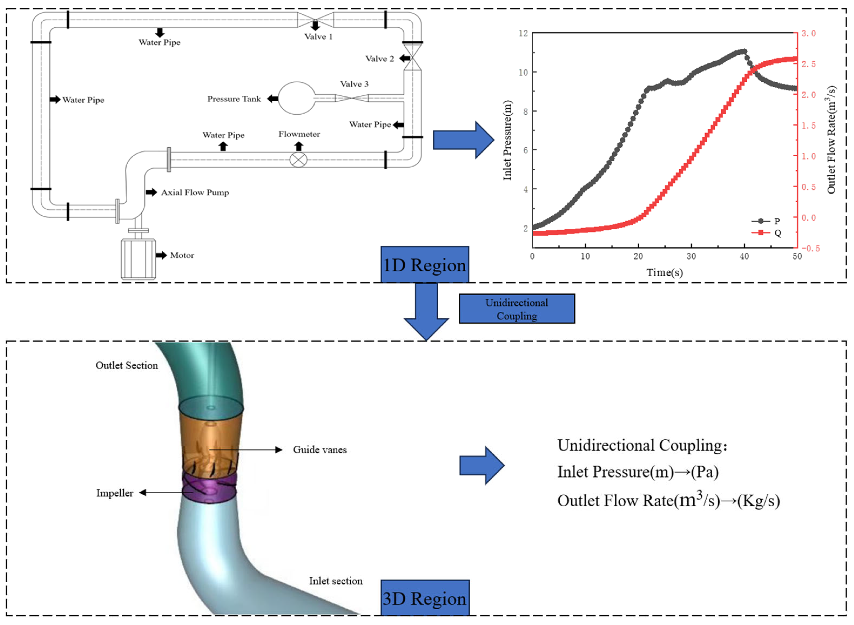
2.2. Numerical Computation Methods and Boundary Conditions

2.2.1. Numerical Computation Methods

The internal flow within the axial flow pump is turbulent. In numerical simulations, the governing equations for the flow field include the continuity equation, momentum equation, and energy equation. These three equations are established based on the principles of the conservation of mass, momentum, and energy [21]. In this study, the fluid is assumed to be incompressible, room-temperature water, so the governing equations consist of the continuity equation and the momentum equation. The addition of the RNG k-ε two-equation turbulence model ensures the closure of the equation system. The RNG k-ε turbulence model uses the renormalization group mathematical method to reconstruct the Navier–Stokes equations and correct the turbulent viscosity. It accounts for turbulent vortices, enabling the model to simulate multi-scale turbulence diffusion (large curvature, strong rotation, high strain rate flow). The relevant equations are as follows:

Mass Conservation Equation:

$${\displaystyle \frac{\partial \rho }{\partial t}}+{\displaystyle \frac{\partial (\rho u_i)}{\partial x_i}}=0$$

(1)

Momentum Conservation Equation:

$${\displaystyle \frac{\partial (\rho u)}{\partial t}}+div(\rho uu)=div(ugrad\hspace{1em}u)-{\displaystyle \frac{\partial \rho }{\partial x}}$$

(2)

$${\displaystyle \frac{\partial (\rho v)}{\partial t}}+div(\rho vu)=div(ugrad\hspace{1em}v)-{\displaystyle \frac{\partial \rho }{\partial x}}$$

(3)

$${\displaystyle \frac{\partial (\rho w)}{\partial t}}+div(\rho wv)=div(ugrad\hspace{1em}w)-{\displaystyle \frac{\partial \rho }{\partial x}}$$

(4)

Turbulent Kinetic Energy (k) Equation:

$${\displaystyle \frac{\partial \left(\rho k\right)}{\partial t}}+{\displaystyle \frac{\partial \left(\rho k{u}_i\right)}{\partial x_i}}={\displaystyle \frac{\partial }{\partial x_j}}\left({\alpha }_k{\mu }_{eff}{\displaystyle \frac{\partial k}{\partial x_j}}\right)+G_k+\rho \epsilon$$

(5)

Turbulent Kinetic Energy Dissipation Rate (ε) Equation:

$${\displaystyle \frac{\partial \left(\rho \epsilon \right)}{\partial t}}+{\displaystyle \frac{\partial \left(\rho \epsilon u_i\right)}{\partial x_i}}={\displaystyle \frac{\partial }{\partial x_j}}\left({\alpha }_{\epsilon }{\mu }_{eff}{\displaystyle \frac{\partial \epsilon }{\partial x_j}}\right)+{C_{1\epsilon }}^{\ast }{\displaystyle \frac{\epsilon }{k}}{G}_k-C_{2\epsilon }\rho {\displaystyle \frac{{\epsilon }^2}{k}}$$

(6)

In the equation, $G_k$ represents the production term of turbulent kinetic energy k, which can be expressed as $G_k={\mu }_t\left({\displaystyle \frac{\partial u_i}{\partial x_j}}+{\displaystyle \frac{\partial u_j}{\partial x_i}}\right){\displaystyle \frac{\partial u_i}{\partial x_j}}$. ${\mu }_{eff}=\mu +{\mu }_t$, ${\mu }_t={\displaystyle \frac{\rho C_{\mu }{k}^2}{\epsilon }}$,$C_{\mu }=0.0845$, α_k and α_ε represent the Prandtl numbers related to the turbulent kinetic energy k and dissipation rate ε, respectively. ${\alpha }_k=1.39$, ${\alpha }_{\epsilon }=1.39$, ${C_{1\epsilon }}^{\ast }=C_{1\epsilon }-{\displaystyle \frac{\eta (1-\frac{\eta }{{\eta }_0})}{1+\beta {\eta }^3}}$, the empirical constant $C_{1\xi }=1.42$, $C_{2\xi }=1.68$, $\eta ={\left(2E_{ij}\times E_{ij}\right)}^{{\displaystyle \frac{1}{2}}}{\displaystyle \frac{k}{\epsilon }}$, $E_{ij}={\displaystyle \frac{1}{2}}\left({\displaystyle \frac{\partial u_i}{\partial x_j}}+{\displaystyle \frac{\partial u_j}{\partial x_i}}\right)$, and ${\eta }_0=4.377$, $\beta =0.012$.

2.2.2. Boundary Conditions

To accurately compute the startup process, the data required for 1D-3D coupling need to be continuously updated with the variation in rotational speed. The one-dimensional calculation process is divided into 101 time steps with a 0.5 s interval, and the startup process data obtained from the 1D calculations are fed back to the 3D flow field for 3D simulation. The boundary conditions for the three-dimensional computational domain are set as follows: pressure inlet (Pa) and mass flow rate outlet (Kg/s). A second-order upwind scheme is employed for interpolation, and the SIMPLEC algorithm is used for solving the equations. Except for the impeller region, all other regions are fixed. The convergence criterion for each simulation is set to 10⁻⁵. The simulation schematic is shown in Figure 2.

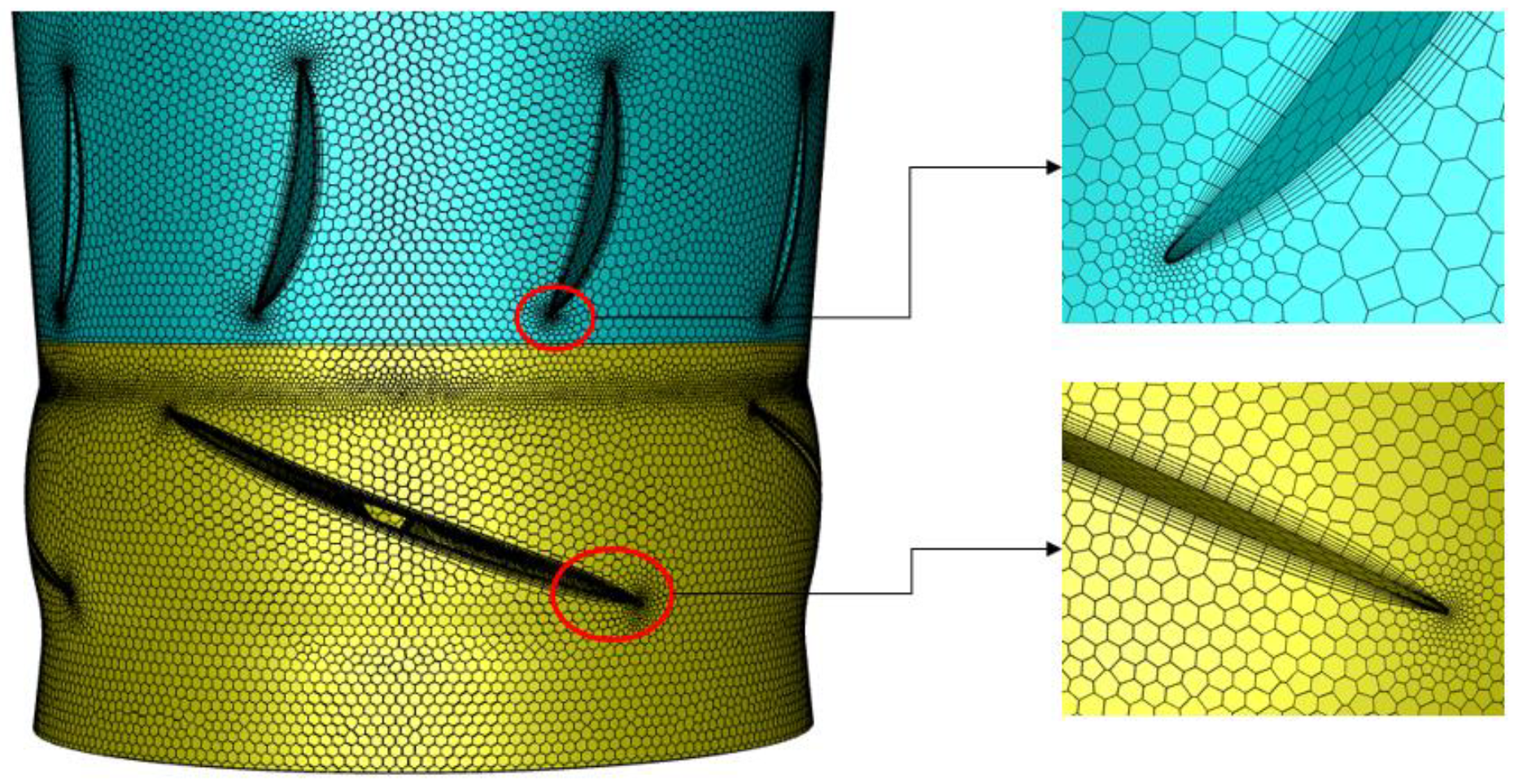
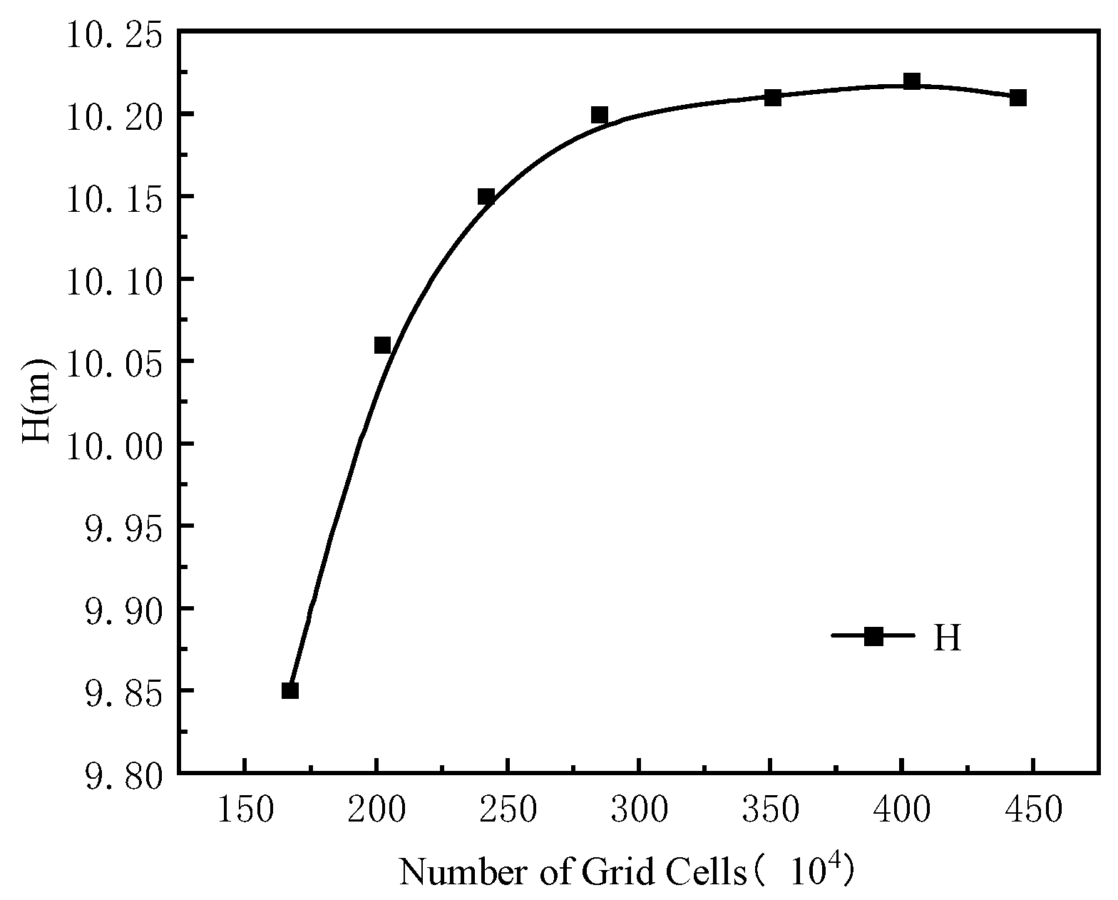
2.3. Mesh Generation

To ensure the accuracy and reliability of the calculation results, polyhedral meshing was performed on the three-dimensional fluid domain of the axial flow pump using ANSYS Fluent Meshing. Boundary layer mesh refinement was applied to the impeller blades and guide vanes. A schematic diagram of the mesh for the main components of the axial flow pump is shown in Figure 3. To verify the impact of the mesh scale on simulation performance, seven different mesh scales were compared. The calculation results are shown in Figure 4. When the head in the results stabilized, the model mesh number was determined to be 2,846,130.

3. Numerical Computation and Results Analysis

3.1. Experimental Validation

To verify the accuracy of the numerical computations, numerical calculations and experimental tests were conducted for seven operating conditions of the axial flow pump model. Figure 5 shows the experimental setup diagram of the axial flow pump model and a comparison of the calculated and experimental values for the pump head and efficiency. The scale ratio between the experimental pump and the model pump is 1:4.7. From the figure, it can be observed that the maximum error between the experimental and calculated values of the flow rate–head curve is 4.25%, and the maximum error between the experimental and calculated values of the flow rate–efficiency curve is 2.5%. Therefore, it is concluded that the model tests and numerical calculations in this study have a high degree of consistency, and the numerical simulation is deemed suitable for this research.

3.2. Effect of the Gate Pre-Opening Angle on Performance

At zero flow, the axial power of the axial flow pump is at its maximum. Therefore, the gate valve on the discharge pipeline must be opened before the pump starts to reduce the startup power. During the startup of the axial flow pump, the gate should not be in the closed position, as this would impose the maximum load on the pump. However, having a larger gate opening is not always better. As the gate pre-opening angle increases, the internal backflow rate during startup also increases, leading to decreased fluid stability within the pump. Therefore, it is necessary to choose an appropriate gate pre-opening angle.

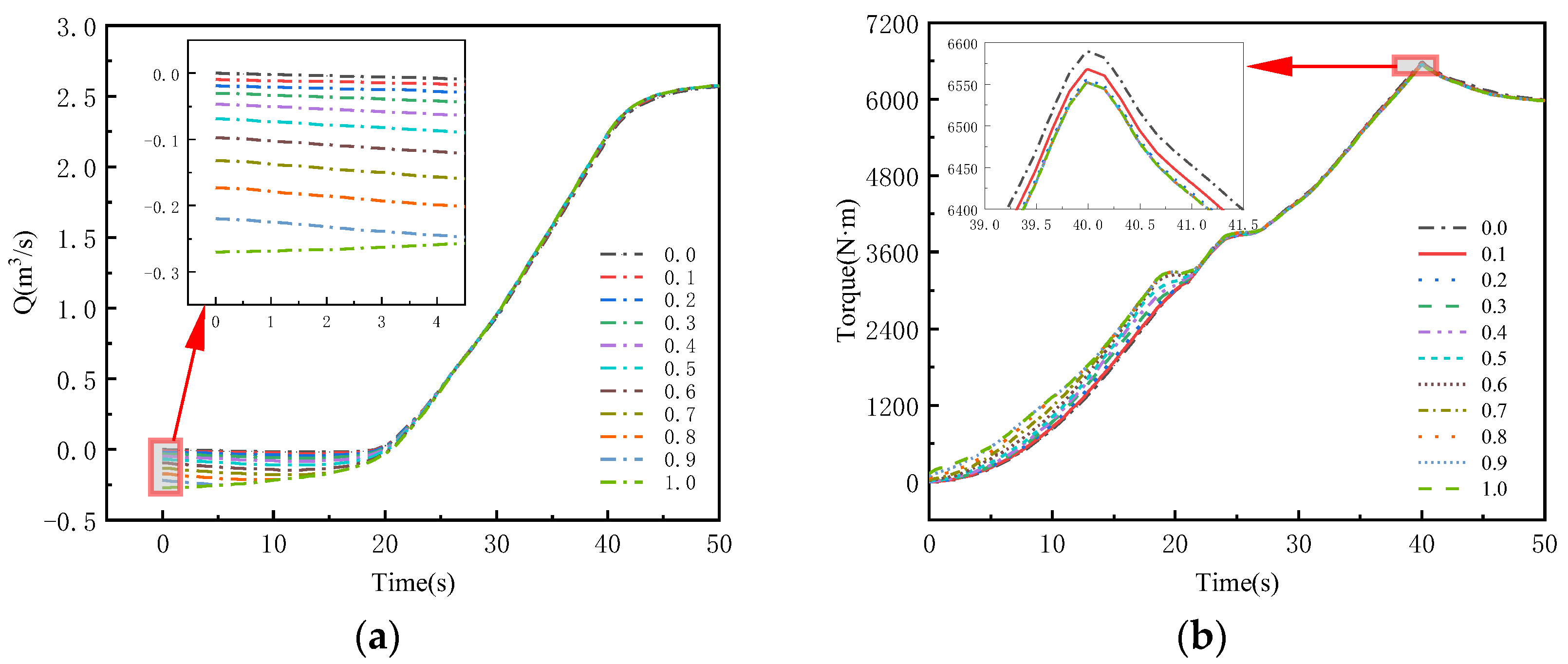
3.2.1. Flow Rate, Torque Calculation, and Analysis

To investigate the effect of the gate pre-opening angle on the pump unit startup, the pump is started with different gate pre-opening angles. To ensure a single variable, the gate opening speed and pump startup time remain constant for each test with different pre-opening angles. In the study, a fully open gate is defined as 1, while a fully closed gate is defined as 0. The gate pre-opening angle is varied from fully closed to fully open, with each experiment conducted at an interval of a 0.1 opening angle. The numerical simulation results are shown in Figure 6.

In Figure 6a, it can be seen that as the gate pre-opening angle increases, the backflow rate of the pump gradually increases. When the gate is fully open and the pump is started, the maximum backflow rate in the pump reaches a peak of 0.2701 m³/s, which is 10.98% of the design flow rate. At 20 s into the pump operation, the backflow situation disappears. However, the change in pump torque differs from the flow rate. As shown in Figure 6b, the startup torque of the pump gradually decreases with an increasing gate pre-opening angle. When the pump reaches its rated speed, the torque inside the pump reaches its maximum value. This is consistent with what is described in Reference [3], where the transient impact during pump startup reaches its peak at the rated speed. The maximum torque of the pump is observed when the gate pre-opening angle is 0, with a maximum torque of 6589.66 N·m, which is 92.41% of the calculated torque. (The torque in this calculation is derived using Equation $T={\displaystyle \frac{9550\times P}{n}}$, where P represents the motor power and n denotes the rated speed of the pump.) The curves of the maximum backflow rate and maximum torque versus the gate pre-opening angle in the experiments are shown in Figure 7.

In Figure 7, it can be seen that when the gate pre-opening angle is 0.2, both the maximum torque and backflow rate during the pump startup are relatively small. The maximum torque is 6555.79 N·m, which is 91.94% of the calculated torque, and the maximum backflow rate is 0.0421 m³/s, which is 1.71% of the design flow rate. After the gate opening angle reaches 0.3, with an increasing pre-opening angle, the maximum torque in the pump gradually stabilizes and is no longer influenced by the opening angle. The maximum torque remains around 6552 N·m, which is 91.88% of the calculated torque. When the gate pre-opening degree is 0.6, the backflow rate within the pump is 0.1449 m³/s, which is 5.89% of the pump’s rated flow rate. Meanwhile, as the gate opening angle increases, the backflow rate in the pump shows a continuous growth trend. When the gate pre-opening angle is 1.0, the backflow rate reaches its maximum value of 0.2701 m³/s, which is 10.98% of the design flow rate.

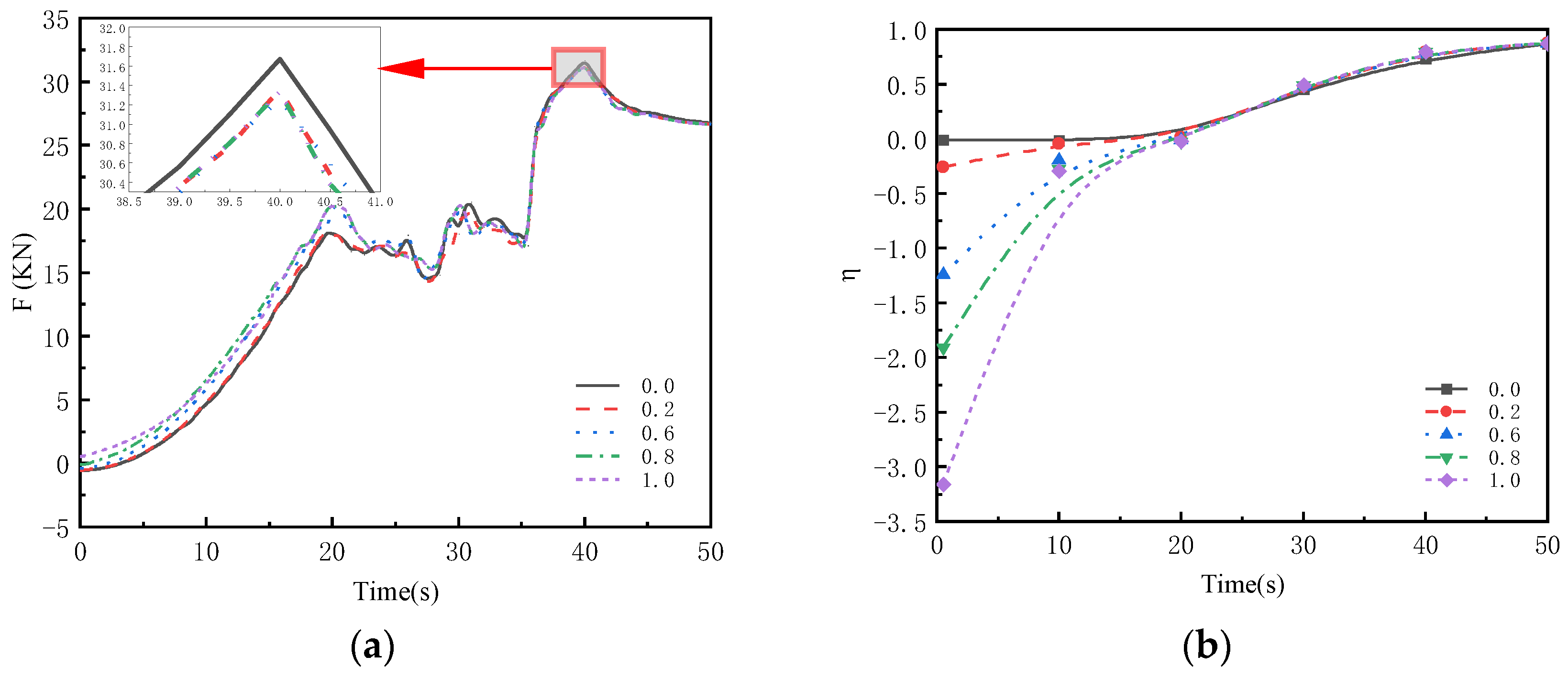
3.2.2. Axial Force, Efficiency Calculation, and Analysis

To further analyze the internal flow conditions of the axial flow pump during startup with different gate pre-opening angles, 1D-3D-coupled simulations were performed based on 1D simulations with gate pre-opening angles of 0.0, 0.2, 0.6, 0.8, and 1.0. Figure 8 shows the axial force curves on the impeller blades of the axial flow pump and the efficiency curves of the pump for different gate pre-opening angles. The efficiency shown in the figure is based on the First Law of Thermodynamics. The calculation is performed using the following formula:

$$\eta ={\displaystyle \frac{\rho gQH}{M\omega }}$$

(7)

In the formula, M represents the torque, and $\omega$ represents the angular velocity of the pump.

From Figure 8a, it can be observed that at 40 s, when the pump reaches its rated speed, the axial force generated by the impeller of the axial flow pump peaks. This is consistent with what is described in Reference [3], where the transient impact during the pump startup reaches its peak at the rated speed. The maximum axial force occurs when the gate opening angle is 0, with a maximum axial force of 31.67 kN, which exceeds the axial force of 18.93% after the pump reaches stable operation. Figure 8b shows that the pump efficiency is inversely proportional to the backflow rate within the pump. As the gate pre-opening angle increases, the backflow rate increases and the pump efficiency decreases. When the gate pre-opening angle is 1.0, the pump efficiency reaches its lowest point at 0.5 s after startup. At a pre-opening angle of 0, the initial efficiency of the pump during startup is 0.

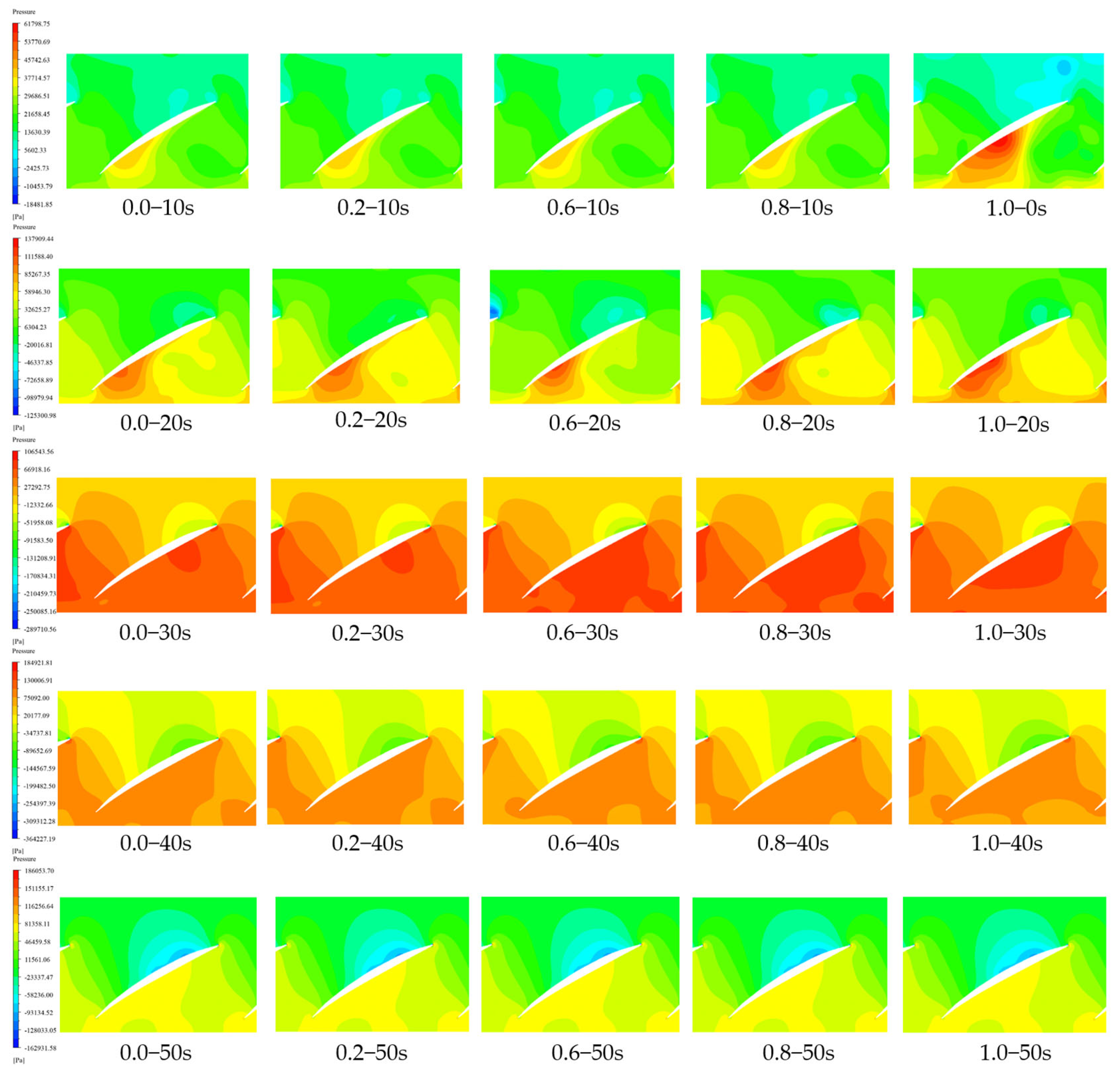
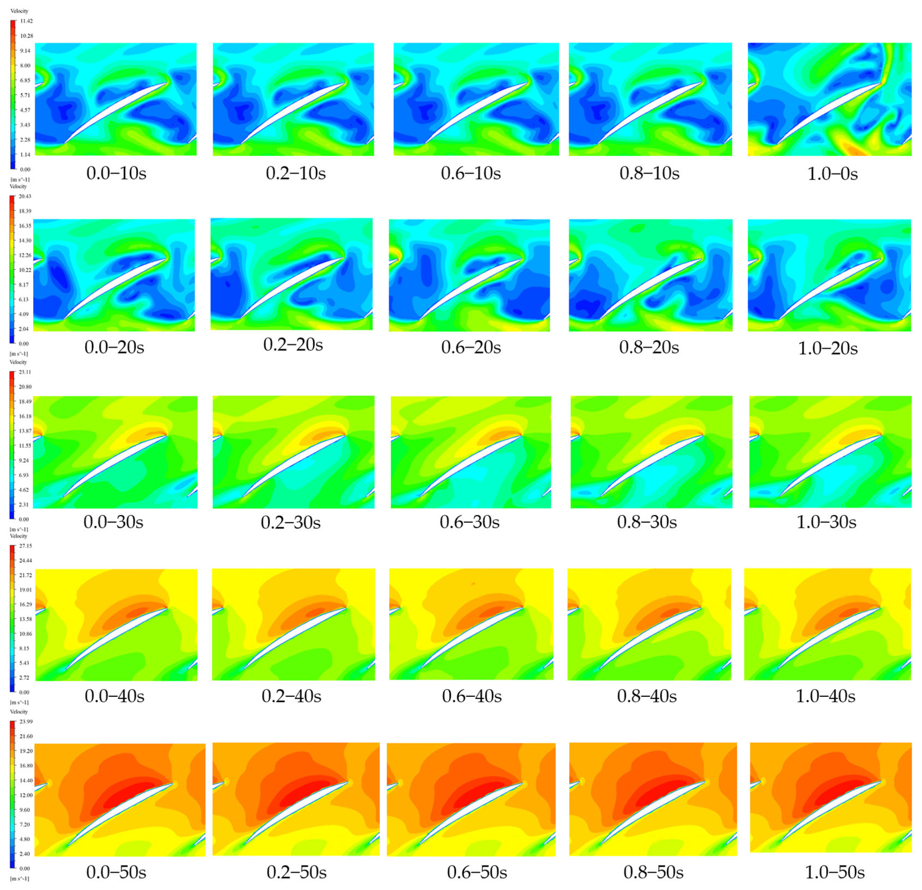
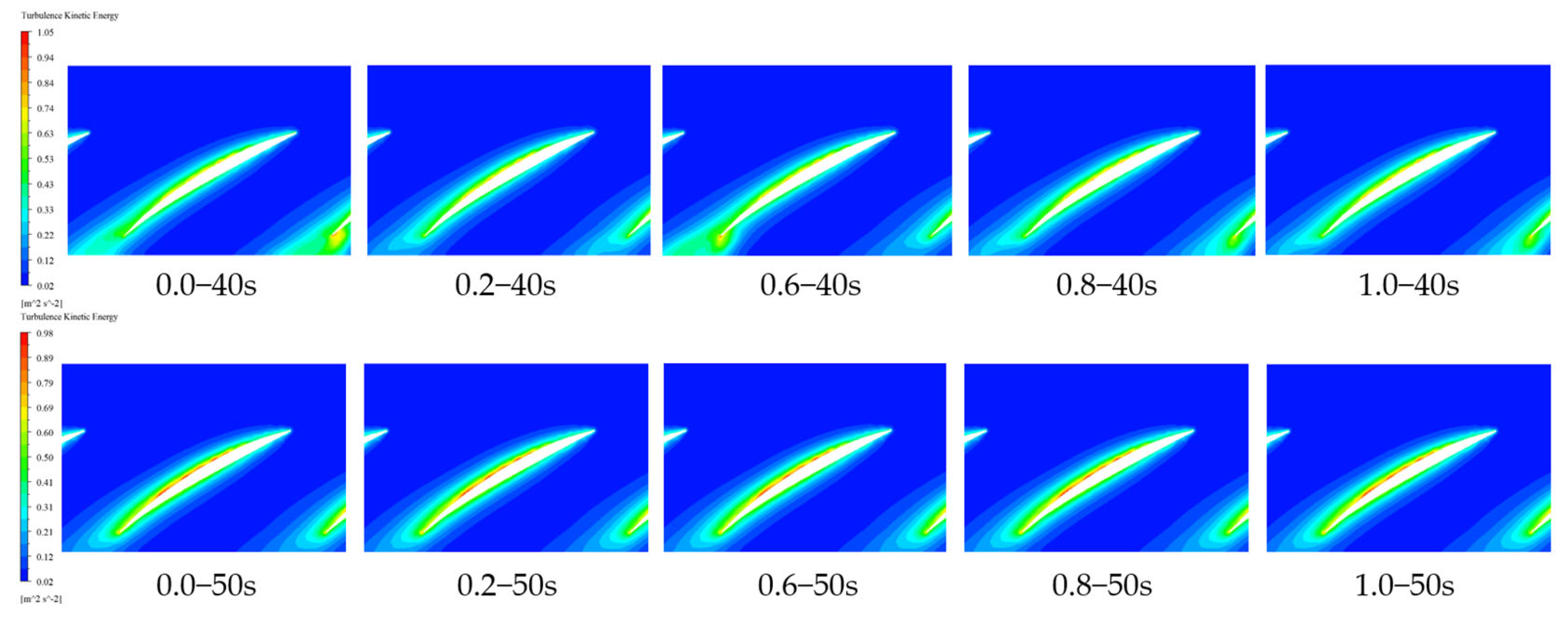
3.2.3. Internal Flow Field Calculation and Analysis

Based on this, further analysis of the internal characteristics of the impeller at a radial coefficient r = 0.5 during the startup process of the axial flow pump is conducted at 10 s, 20 s, 30 s, 40 s, and 50 s. The schematic diagram at the radial coefficient r = 0.5 is shown in Figure 9. Figure 10, Figure 11 and Figure 12 show the conditions at different times, with 0.0–10 s representing the pump running from 0 to 10 s with a gate pre-opening angle of 0.

Figure 10 and

Table 2. Dimensionless Pressure Extremes at r = 0.5 of the Impeller at Different Times and Various Gate Pre-opening Degrees.

	Opening Degree	0	0.2	0.6	0.8	1.0
Time
10 s		−0.5795	−0.5753	−0.4336	−0.3787	−0.3811
20 s		0.1372	0.2442	0.2049	0.3731	0.3811
30 s		0.0497	0.0427	0.0670	0.0515	0.0515
40 s		0.8520	0.7934	0.8378	0.7590	0.7590
50 s		0.8652	0.8635	0.8638	0.8633	0.8633

and

Table 3. Dimensionless Negative Pressure Extremes at r = 0.5 of the Impeller at Different Times and Various Gate Pre-opening Degrees.

	Opening Degree	0	0.2	0.6	0.8	1.0
Time
10 s		−0.8714	−0.9010	−0.9094	−0.8478	−0.8149
20 s		−0.2991	−0.1980	0.2549	0.0910	−0.2069
30 s		1.6998	1.9014	1.7051	1.8653	1.8653
40 s		2.6343	2.5752	2.6477	2.5894	2.5894
50 s		0.6822	0.6407	0.6523	0.6317	0.6317

show the pressure contour maps of the axial flow pump impeller at a radial coefficient r = 0.5 and the corresponding maximum and minimum values of positive and negative pressure. From these figures and tables, it can be observed that the low-pressure zone is mainly concentrated at the blade tip and the inlet of the impeller. During the first 20 s of pump startup, the pressure peak is found under conditions of large gate opening (gate pre-opening angles of 0.8 and 1.0). When the pump reaches its rated speed, the maximum pressure occurs with a gate pre-opening angle of 0, with a maximum dimensionless pressure of 0.8520, followed by a pre-opening angle of 0.6, where the dimensionless pressure peak reaches 0.8378. As the pump startup reaches its rated speed, the high-pressure zone inside the impeller gradually increases. When the pump reaches its rated speed (at 40 s), the pressure distribution inside the impeller becomes uniform. When all the pump valves are fully open (At 50 s), the maximum pressure inside the pump starts to stabilize after the gate pre-opening angle reaches 0.6. At pre-opening angles of 0.8 and 1.0, the peak values of positive and negative pressures inside the pump become equal.

Let x be the gate pre-opening angle, y be the running time, a be the non-dimensionalized positive pressure, and b be the non-dimensionalized negative pressure. The function relationship of pressure as a function of x and y is obtained through fitting.

Positive Pressure: Correlation coefficient of 0.99.

$$\begin{array}{c}a=-38.02y^4+(1.95x+114.47)y^3+(-0.14x^2-3.91x-119.37)y^2+(0.26x^3\\ -0.19x^2+2x+51.38)y+(-0.48x^4+0.57x^3-0.05x^2-0.11x-7.61)\end{array}$$

(8)

Negative Pressure: Correlation coefficient of 0.99.

$$\begin{array}{c}b=-20.48y^3+(-0.41x+38.77)y^2+(0.51x^2-0.07x-16.8)y+\\ (-0.38x^3-0.1x^2+0.46x+1.12)\end{array}$$

(9)

In the formula $y={\displaystyle \frac{y^{\prime }}{40}}$, $y^{\prime }$ represents the running time in seconds (s). The pressure is expressed in a dimensionless form, as follows:

$$a={\displaystyle \frac{P-P^{\prime }}{P^{\prime }}}=b$$

(10)

$$P^{\prime }=\rho gH$$

(11)

In the formula, P represents the maximum instantaneous pressure at that location, in Pascals (Pa). The internal fluid is water, with a density of $\rho =998.2\mathrm{kg}/{\mathrm{m}}^3$. Based on the fitted relationship, the maximum pressure at the cross-section with a radial impeller coefficient of r = 0.5 under different operating conditions can be obtained.

Figure 11 and

Table 4. Dimensionless Velocity Extremes at r = 0.5 of the Impeller at Different Times and Various Gate Pre-opening Degrees.

	Opening Degree	0	0.2	0.6	0.8	1.0
Time
10 s		0.2343	0.3647	0.4574	0.5742	0.6624
20 s		0.1536	0.1941	0.4866	0.3450	0.3539
30 s		0.1210	0.0935	0.0914	0.0715	0.0715
40 s		−0.0122	−0.0251	−0.0137	−0.0257	−0.0257
50 s		−0.1270	−0.1270	−0.1268	−0.1271	−0.1271

show the velocity contour map and the corresponding velocity extremes at the radial coefficient r = 0.5 for the axial flow pump impeller. From the figures and table, it can be observed that the high-speed zone of the fluid is concentrated at the blade tip and the inlet of the impeller. During the initial startup of the pump, as the gate pre-opening angle increases, the fluid velocity distribution inside the pump becomes increasingly uneven. This indicates that the flow inside the pump becomes progressively turbulent with an increasing gate pre-opening angle, which is due to the increased internal recirculation. When the pump is started with the valve closed and reaches the rated speed at 40 s, the maximum flow speed is 27.15 m/s, which is 1.22% of the outlet speed. For a gate opening angle of 0.6, the maximum speed at 40 s is 27.11 m/s, which is 1.37% of the outlet speed. At gate pre-opening angles of 0.8 and 1.0, the maximum speed inside the pump at rated speed is 26.78 m/s, which is a decrease of approximately 1.38% compared to the closed valve start. After reaching stable operation, the flow speed is reduced to 23.99 m/s, which is 12.71% of the outlet speed, a decrease of about 13.15% compared to the maximum flow speed at the closed valve start. At this point, the speed distribution inside the pump is more uniform compared to the distribution before reaching the rated speed, with a clearer boundary between high-speed and low-speed zones.

Let x be the gate pre-opening angle, y be the running time, and c be the non-dimensionalized velocity. The function relationship of velocity as a function of x and y is obtained through fitting.

Velocity: Correlation coefficient of 0.97.

$$\begin{array}{c}c=0.37y^3+(0.76x-0.99)y^2+(0.21x^2-1.77x+0.44)y+\\ (0.08x^3-0.15x^2+0.98x+0.17)\end{array}$$

(12)

In the formula, y and $y^{\prime }$ are as defined previously. The velocity is expressed in a dimensionless form, as follows:

$$c={\displaystyle \frac{u-u_2}{u_2}}$$

(13)

$$u_2={\displaystyle \frac{n\pi D_2}{60}}$$

(14)

In the formula, u represents the maximum instantaneous velocity at the cross-section with a radial impeller coefficient of r = 0.5 under any operating condition in the model. Based on the fitted relationship, the maximum velocity at the cross-section with a radial impeller coefficient of r = 0.5 under other operating conditions can be obtained.

Figure 12 and

Table 5. Turbulent Kinetic Energy Extremes at r = 0.5 of the Impeller at Different Times and Various Gate Pre-opening Degrees.

	Opening Degree	0	0.2	0.6	0.8	1.0
Time
10 s		0.4252	0.4300	0.5413	0.6564	0.9470
20 s		1.7640	2.0214	1.7903	1.5897	1.6991
30 s		1.0212	1.0632	0.9904	1.0667	1.0667
40 s		0.8944	0.8916	1.0237	1.0464	1.0464
50 s		0.9792	0.9815	0.9803	0.9813	0.9813

show the turbulence kinetic energy contour map and the corresponding turbulence kinetic energy extremes at the radial coefficient r = 0.5 for the axial flow pump impeller. From the figures and table, it can be observed that within the first 20 s of pump startup, the turbulence kinetic energy distribution inside the pump is uneven, with vortices forming at the blade tips. During this period, the fluid stability inside the pump is relatively poor. At 20 s into the startup, as the gate opening angle increases, the turbulence kinetic energy also increases. The maximum turbulence kinetic energy occurs with a gate pre-opening angle of 0.2, reaching 2.0214 m²/s². At a gate pre-opening angle of 0.8, the maximum turbulence kinetic energy is 1.5897 m²/s², which is a 27.16% decrease compared to the 0.2 opening. With a gate pre-opening angle of 1.0, the fluid stability inside the pump is relatively poor throughout the startup process, with a 6.88% increase in turbulence kinetic energy compared to the 0.8 opening. After 30 s of startup, the turbulence kinetic energy distribution inside the pump becomes more uniform, with a smooth streamline from the impeller inlet to the outlet, indicating improved fluid stability.

Let x be the gate pre-opening angle, y be the running time, and d be the turbulence kinetic energy. The function relationship of turbulence kinetic energy as a function of x and y is obtained through fitting.

Turbulence kinetic energy: Correlation coefficient of 0.98.

$$\begin{array}{c}d=-33.95y^4+(-6.95x+115.95)y^3+(2.19x^2+14.55x-139.15)y^2+\\ (-2.5x^3+0.05x^2-9.78x+67.46)y+(0.32x^4+2.16x^3-2.5x^2+2.7x-9.47)\end{array}$$

(15)

Based on the fitted relationship, the maximum turbulent kinetic energy at the cross-section with a radial impeller coefficient of r = 0.5 under other operating conditions can be obtained.

Figure 13 shows the variation curves of the maximum pressure difference, velocity, and turbulent kinetic energy at r = 0.5 of the impeller under different gate pre-opening degrees during pump startup at 10 s, 20 s, 30 s, 40 s, and 50 s. By examining the contour plots in Figure 11, Figure 12 and Figure 13, it can be observed that when the pump starts with a gate pre-opening degree of 0.6, the internal pressure difference is minimized, which is beneficial in reducing the forces on the impeller. In the early stage of pump startup (within the first 20 s), the internal pressure difference is the highest when the gate pre-opening degree is 0.8 and 1.0, being 28.96% higher than at 0.6. As shown in the backflow variation curve in Figure 6a, backflow occurs within the pump during the first 20 s, with the highest backflow occurring at gate pre-opening degrees of 0.8 and 1.0, resulting in the maximum internal pressure difference and poor flow stability. The velocity variation follows a similar pattern as the pressure difference, with the maximum velocity occurring at 0.8 and 1.0 degrees in the first 20 s, being 14.62% higher than at 0.6. The higher pressure difference leads to an increase in flow velocity, contributing to poor fluid stability within the pump. Turbulent kinetic energy fluctuations are most noticeable when the pump is started with a gate pre-opening degree of 0.2. In summary, when the pump is started with a gate pre-opening degree of 0.6, the internal flow conditions are relatively better.

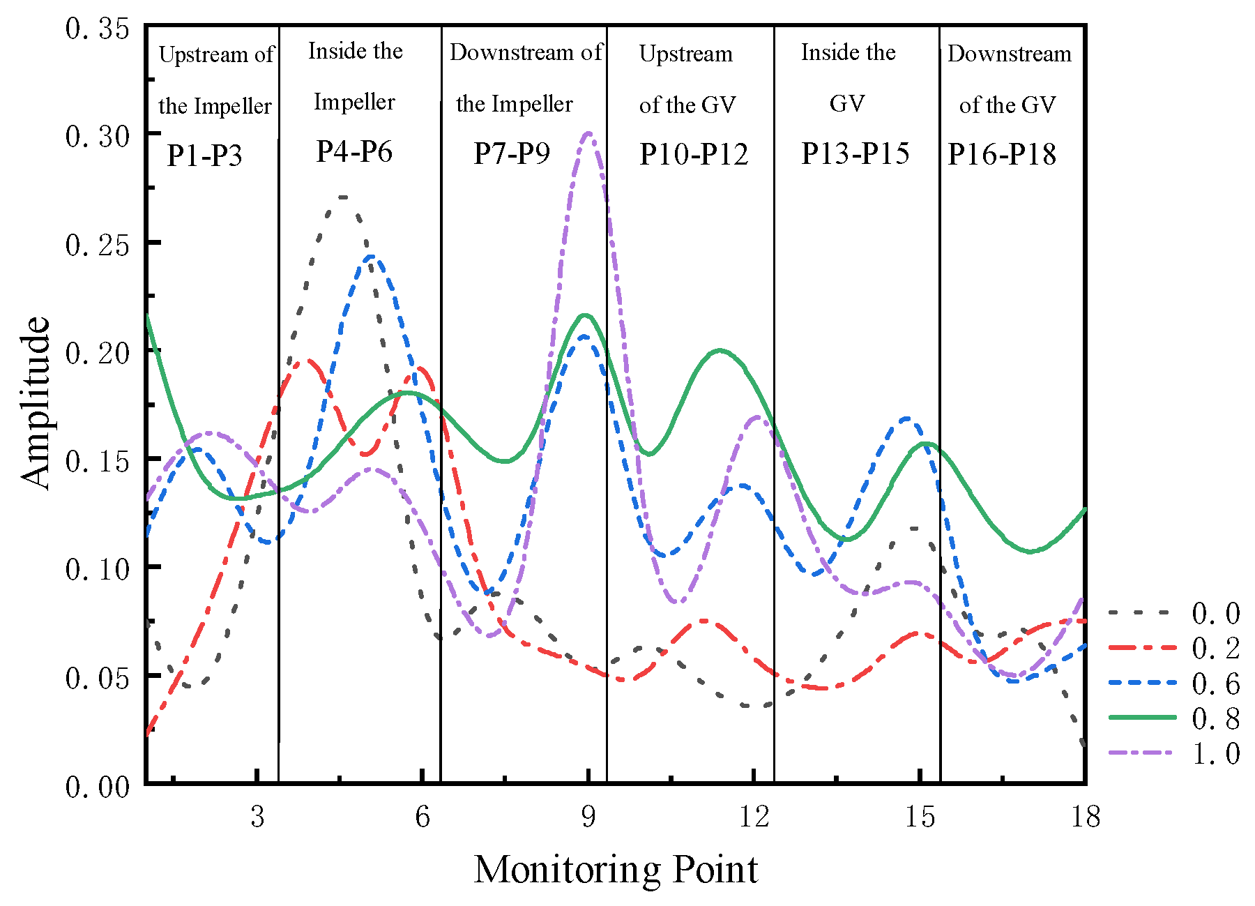
3.3. Analysis of the Effect of Gate Pre-Lift on Pressure Fluctuation Characteristics

To further investigate the impact of different gate pre-lift settings on the pressure fluctuation characteristics within the axial flow pump, pressure fluctuations were measured at 10 s after pump startup under various pre-lift conditions. At this time, the pump operated at a rotational speed of 187.5 rpm. Pressure distribution was recorded every 2° during the impeller’s rotation, with a time step of 0.001778 s. The data analyzed were collected after the pump had completed four stable revolutions. To monitor the pressure fluctuations within the pump, measurement points were radially arranged at several cross-sections: the inlet of the impeller (P1–P3), the mid-section of the impeller (P4–P6), the outlet of the impeller (P5–P9), the inlet of the guide vanes (P10–P12), the mid-section of the guide vanes (P13–P15), and the outlet of the guide vanes (P16–P18). The distribution of these measurement points is illustrated in Figure 14.

In this study, pressure fluctuation characteristics are represented using the pressure coefficient. The formula for the pressure coefficient is as follows:

$$C_p={\displaystyle \frac{P-\overline{P}}{0.5\rho u_2^2}}$$

(16)

In the formula, P represents the instantaneous pressure value, $\overline{P}$ denotes the average pressure value, $\rho$ is the fluid density, and $u_2$ is the circumferential velocity at the impeller outlet.

Figure 15 and

Table 6. Statistical Characteristics of Pressure Fluctuations at Different Monitoring Points Inside the Impeller.

Pre-Opening Degree	Monitoring Point	Fundamental Frequency	Amplitude	Relative Amplitude	Subharmonic Frequency	Amplitude	Relative Amplitude
0.0	P4	3.125	0.256	0.850	12.500	0.044	0.415
	P5	3.125	0.301	1.000	12.500	0.081	0.764
	P6	3.125	0.028	0.093	12.500	0.027	0.255
0.2	P4	3.125	0.227	0.754	28.125	0.018	0.170
	P5	9.375	0.111	0.369	15.625	0.056	0.528
	P6	3.125	0.240	0.797	18.750	0.021	0.198
0.6	P4	3.125	0.129	0.429	12.500	0.064	0.604
	P5	3.125	0.288	0.957	12.500	0.032	0.302
	P6	3.125	0.171	0.568	12.500	0.065	0.613
0.8	P4	3.125	0.137	0.455	15.625	0.041	0.387
	P5	3.125	0.174	0.578	21.875	0.020	0.189
	P6	3.125	0.187	0.621	15.625	0.106	1.000
1.0	P4	3.125	0.112	0.372	12.500	0.052	0.491
	P5	3.125	0.158	0.525	28.125	0.009	0.085
	P6	6.250	0.125	0.415	12.500	0.081	0.764

illustrate the variations in pressure pulsation at monitoring points within the impeller. In Table 6, the relative amplitude represents the ratio of the amplitude at a given point to the maximum amplitude among the fundamental and harmonic frequencies. By examining Figure 14 and Table 6, it can be observed that, except for the cases where the gate opening is 0.2 and 1.0, the fundamental frequency of pressure pulsation at all points corresponds to the rotational frequency. The pressure pulsation amplitude is minimal at gate openings of 0.8 and 1.0, with the maximum relative amplitudes being 0.621 and 0.525, respectively. Compared to the maximum amplitudes at gate openings of 0.0 and 0.2, the maximum amplitudes at 0.8 are lower by 41.00% and 28.51%, respectively. At gate openings of 0.0, 0.2, and 0.6, there is a significant variation in pressure amplitude from the blade tip to the hub, with the maximum relative amplitude difference being 0.907 at an opening of 0.0, indicating an uneven pressure distribution. However, at a gate opening of 0.8, the maximum relative amplitude difference is reduced to 0.166, suggesting a more uniform pressure distribution from the blade tip to the hub.

Figure 16 presents the pressure pulsation amplitude curves at various plane monitoring points for different gate opening degrees. Overall, at a gate opening of 0.2, the maximum amplitude is the smallest, measuring 0.240. This is followed by a gate opening of 0.8, where the maximum amplitude is 0.261, which is 8.70% higher than at 0.2. At a gate opening of 1.0, the maximum amplitude reaches 0.412, representing an increase of 57.96% compared to the maximum amplitude at 0.8. Combining this with the data from Figure 14, it can be concluded that when the gate opening is 0.8, the amplitude inside the pump is relatively smaller upon pump restart.

In summary, the gate opening degree significantly affects both the internal and external characteristics of the pump. Regarding the external characteristics, after the gate opening reaches 0.3, the maximum torque within the pump stabilizes with increasing pre-opening degrees, while the recirculation flow within the pump shows a continuous increasing trend with larger gate openings. Initially, as the gate pre-opening degree increases, the pump’s efficiency decreases. Concerning the internal characteristics, considering pressure, velocity, and turbulence intensity, the fluid stability inside the pump is relatively better at a gate pre-opening degree of 0.8 compared to other pre-opening degrees. For pressure pulsation, at large gate openings (i.e., pre-opening degrees greater than 0.6), the internal pressure distribution is more uniform, and the pressure peaks are smaller compared to those at smaller gate openings. However, as the gate opening increases, the recirculation within the pump also increases, which significantly impacts fluid stability and pump efficiency. Overall, the pressure pulsation amplitude is relatively smaller at a pre-opening degree of 0.8.

4. Conclusions

This paper focuses on a vertical axial flow pump and employs a 1D-3D coupling method to study the effects of different gate pre-lift openings during pump start-up on the internal and external flow characteristics of the axial flow pump. The following conclusions are drawn:

(1)

During the startup of the axial flow pump at different gate pre-opening degrees, backflow persists for the first 20 s, and the backflow rate within the pump increases with the gate pre-opening degree. When the gate pre-opening degree is 0.6, it is 5.89% of the pump’s rated flow rate. When the valve is fully open and the pump is restarted, the maximum backflow rate reaches 10.98% of the rated flow rate. This results in poor fluid stability within the pump, and the efficiency changes negatively due to the influence of the backflow rate.

(2)

At the moment the axial flow pump reaches its rated speed during startup, the axial force peaks. However, the gate pre-opening degree has little impact on the axial force during startup, as the curves of axial force versus time are almost identical.

(3)

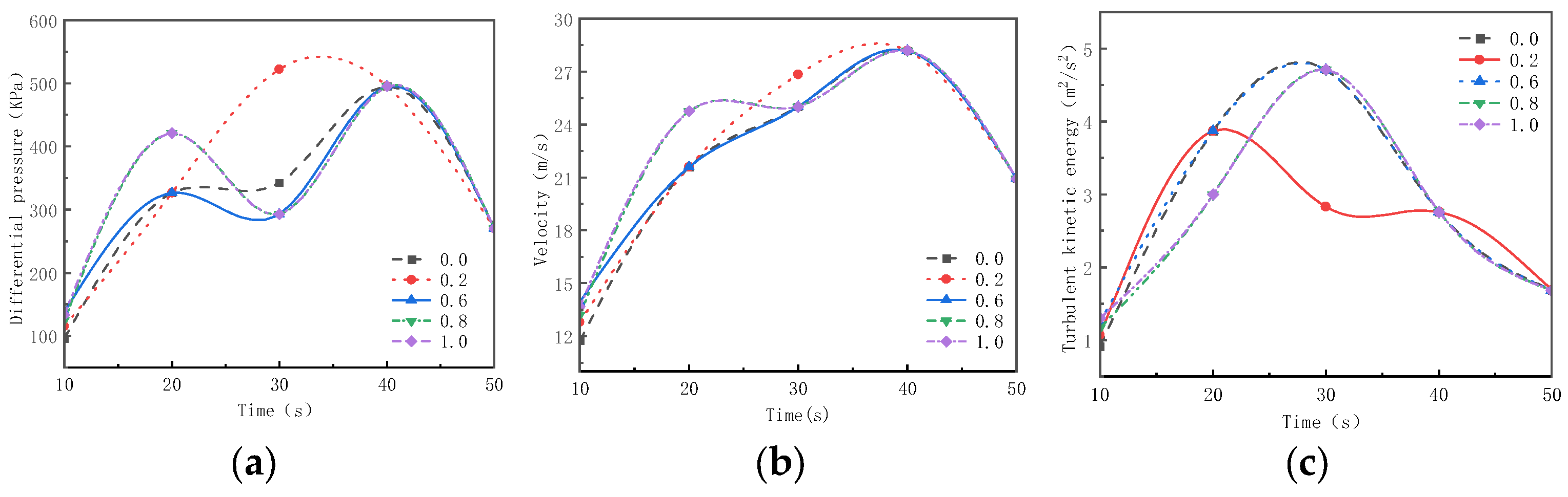
During the pump startup process, when starting with a gate pre-opening degree of 0.6, the internal pressure difference of the pump is minimized. Within the first 20 s of startup, the internal pressure difference in the impeller is greatest with gate pre-opening degrees of 0.8 and 1.0, which is 28.96% higher than at 0.6. The flow velocity is also 14.62% higher compared to that of the 0.6 degree opening. Therefore, the internal flow conditions of the pump are relatively better when starting with a gate pre-opening degree of 0.6 compared to other degrees.

(4)

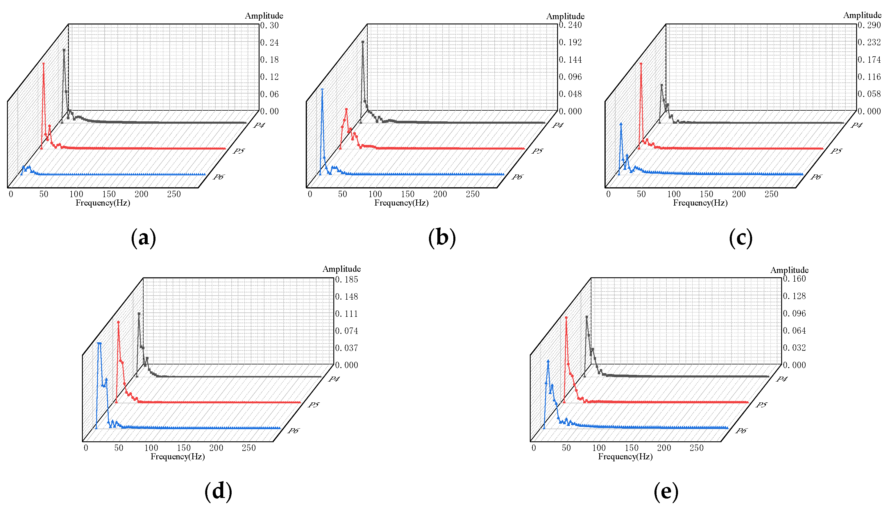
During the pump startup process, with gate pre-opening degrees of 0.8 and 1.0, the initial pressure fluctuation amplitude within the pump is minimal. The relative amplitudes are only 0.621 and 0.525, respectively, which are 41.00% and 28.51% lower than the maximum amplitudes corresponding to 0 and 0.2 degrees. In summary, the peak pressure inside the pump is minimized when the valve pre-opening degree is around 0.8, while the pressure difference and flow velocity are relatively lower at a pre-opening degree of 0.6. It is recommended to start the pump with a valve pre-opening degree of around 0.6 to 0.8.

References

1. Meng, F.; Qin, Z.J.; Li, Y.J.; Chen, J. Investigation of Transient Characteristics of a Vertical Axial-Flow Pump with Non-Uniform Suction Flow. Machines 2022, 10, 855. [Google Scholar] [CrossRef]
2. Jing, R.; He, X.J. Overview of axial flow pump and its application. Gen. Mach. 2014, 147, 86–89. [Google Scholar]
3. Fu, S.F.; Zheng, Y.; Kan, K.; Chen, H.X.; Han, X.X.; Liang, X.L.; Liu, H.W.; Tian, X.Q. Numerical simulation and experimental study of transient characteristics in an axial flow pump during start-up. Renew. Energy 2020, 146, 1879–1887. [Google Scholar] [CrossRef]
4. Hu, C.Y.; Zhang, X.W.; Tang, F.P.; Xv, X.D.; Huang, C.B.; Jin, L. Influence of Overflow Orifice Diameter on the Transient Process of Axial Flow Pump System. J. Trans. Chin. Soc. Agric. Mach. 2023, 54, 181–191. [Google Scholar]
5. Liu, Y.F.; Zhou, D.Q.; Zheng, Y.; Zhang, H.S.; Xu, J.Y. Numerical simulation of starting process of axial flow pump with quick-stop gate. J. South North Water Divers. Water Sci. Technol. 2017, 15, 167–172. [Google Scholar]
6. Zhang, L.J.; Wang, S.; Yin, G.J.; Guan, C.N. Fluid–structure interaction analysis of fluid pressure pulsation and structural vibration features in a vertical axial pump. Adv. Mech. Eng. 2019, 11, 168781401982858. [Google Scholar] [CrossRef]
7. Guo, Y.L.; Yang, C.X.; Wang, Y.; Lv, T.Z.; Zhao, S. Study on Inlet Flow Field Structure and End-Wall Effect of Axial Flow Pump Impeller under Design Condition. Energies 2022, 15, 4969. [Google Scholar] [CrossRef]
8. Zhang, X.W.; Tang, F.P.; Liu, C.; Shi, L.J.; Liu, H.Y.; Sun, Z.Z.; Hu, W.Z. Numerical Simulation of Transient Characteristics of Start-Up Transition Process of Large Vertical Siphon Axial Flow Pump Station. Front. Energy Res. 2021, 9, 706975. [Google Scholar] [CrossRef]
9. Song, Y.C. Research on Flow Mechanism of Transition Process of Pumped Storage Unit Based on Three-Dimensional Coupling. Master’s Thesis, Harbin Institute of Technology, Harbin, China, 2022. [Google Scholar]
10. Liu, Y.Z. Three-Dimensional Coupling Simulation Analysis of Multi-Cylinder Diesel Engine Intake and Exhaust System. Master’s Thesis, Harbin Engineering University, Harbin, China, 2020. [Google Scholar]
11. Fu, X.L.; Li, D.Y.; Wang, H.J.; Li, Z.G.; Zhao, Q.; Wei, X.Z. One- and three-dimensional coupling flow simulations of pumped-storage power stations with complex long-distance water conveyance pipeline system. J. Clean. Prod. 2021, 315, 128–228. [Google Scholar] [CrossRef]
12. Wang, S. Flow Field Analysis and Performance Optimization of Airflow Transmission Pipeline of Five-Stroke Engine. Master’s Thesis, Chongqing University of Technology, Chongqing, China, 2023. [Google Scholar]
13. Liu, D.M.; Zhang, X.X.; Yang, Z.Y.; Liu, K.; Cheng, Y.G. Evaluating the pressure fluctuations during load rejection of two pump-turbines in a prototype pumped-storage system by using 1D-3D coupled simulation. Renew. Energy 2021, 171, 1276–1289. [Google Scholar] [CrossRef]
14. Liu, K.; Liu, Z.R.; Yang, Z.Y.; Zhang, X.X.; Tai, R.; Cheng, Y.G. Evolution and influence of pump-turbine cavitation during load rejection transients of a pumped-storage plant. J. Hydraul. Res. 2022, 60, 527–542. [Google Scholar] [CrossRef]
15. Lv, J.W.; Fu, X.L.; Li, D.Y.; Wang, H.J.; Wei, X.Z. Instability mechanism of pump power-trip of ultra-high head pump turbines. J. Hydroelectr. Eng. 2023, 11, 11–20. [Google Scholar]
16. Tang, M.J.; Cheng, Y.G.; Liu, D.M.; Chen, H.; Liu, K. FSI simulation of a high-head pump-turbine during load rejection process. J. Phys. Conf. Ser. 2024, 2752, 012198. [Google Scholar] [CrossRef]
17. Cheng, L.; Zhang, K.Y.; Zhang, Y.L.; Jia, X.Q. Effect on Starting Modes on Centrifugal Pump Performance. Processes 2022, 10, 2362. [Google Scholar] [CrossRef]
18. Zhang, X.; Jiang, Y.; Song, X.; Tang, F.; Dai, J.; Yang, F.; Wang, H.; Shi, L. Investigation on the Influence of Flap Valve Area on Transition Process of Large Axial Flow Pump System. J. Mar. Sci. Eng. 2023, 11, 326. [Google Scholar] [CrossRef]
19. Zheng, F.C.; Zhang, X.P.; Chen, T.R.; Huang, B.; Xu, J.; Wang, G.Y. Strong transient characteristics in axial flow waterjet pump during rapid starting period with special emphasis on saddle zone. Ocean Eng. 2023, 269, 113506. [Google Scholar] [CrossRef]
20. Xuan, Y.F.; Zhu, G.J.; Luo, X.Q.; Wang, Y.; Wang, L.K. Experimental Study on the Stability of Mixed-Flow Pump During Segmented Start-Up Process. Arab. J. Sci. Eng. 2024. prepublish. [Google Scholar] [CrossRef]
21. Zhang, X. Study on Flow-Induced Vibration of Low-Specific-Speed Centrifugal Pump Based on Fluid-Structure Interaction. Master’s Thesis, Zhejiang Sci-Tech University, Hangzhou, China, 2016. [Google Scholar]
Figure 1. Schematic Diagram of the Axial Flow Pump Water Model and Valve. (a) Schematic Diagram of the Axial Flow Pump Water Model; (b) Schematic Diagram of the Gate Valve Model.
Processes 12 01984 g001
Figure 2. Schematic Diagram of 1D-3D Coupled Simulation.
Processes 12 01984 g002
Figure 3. Schematic Diagram of the Mesh for Main Components of the Axial Flow Pump.
Processes 12 01984 g003
Figure 4. Schematic Diagram of Mesh Independence Verification.
Processes 12 01984 g004
Figure 5. Experimental Validation of the Model Pump. (a) Schematic Diagram of Axial Flow Pump Experiment Setup; (b) Comparison of Calculated and Experimental Values.
Processes 12 01984 g005
Figure 6. Torque, Flow Rate, and Efficiency vs. Time Curves. (a) Flow Rate vs. Time Plot; (b) Torque vs. Time Plot.
Processes 12 01984 g006
Figure 7. Maximum Backflow Rate and Maximum Torque vs. Pre-Opening Degree.
Processes 12 01984 g007
Figure 8. Axial Force and Efficiency of the Impeller vs. Time at Different Gate Openings. (a) Axial Force vs. Time Plot; (b) Efficiency vs. Time Plot.
Processes 12 01984 g008
Figure 9. At Radial Coefficient r = 0.5 of the Impeller.
Processes 12 01984 g009
Figure 10. Pressure Variation at Different Times for Different Gate Pre-Opening Degrees at r = 0.5 of the Impeller.
Processes 12 01984 g010
Figure 11. Velocity Variation at Different Times for Different Gate Pre-Opening Degrees at r = 0.5 of the Impeller.
Processes 12 01984 g011
Figure 12. Turbulent Kinetic Energy Variation at Different Times for Different Gate Pre-Opening Degrees at r = 0.5 of the Impeller.
Processes 12 01984 g012aProcesses 12 01984 g012b
Figure 13. Time Variation Curves of Various Parameters at r = 0.5 of the Impeller Under Different Gate Pre-Opening Degrees. (a) Pressure Difference–Time Variation Curve; (b) Flow Velocity–Time Variation Curve; (c) Turbulent Kinetic Energy–Time Variation Curve.
Processes 12 01984 g013
Figure 14. Distribution of Monitoring Points.
Processes 12 01984 g014
Figure 15. Frequency Domain Plot of Pressure Pulsations Inside the Axial Pump Impeller. (a) Pre-Opening Degree 0.0; (b) Pre-Opening Degree 0.2; (c) Pre-Opening Degree 0.6; (d) Pre-Opening Degree 0.8; (e) Pre-Opening Degree 1.0.
Processes 12 01984 g015
Figure 16. Pressure Pulsation Amplitudes at Monitoring Points on Various Planes.
Processes 12 01984 g016