Dilation Potential Analysis of Low-Permeability Sandstone Reservoir under Water Injection in the West Oilfield of the South China Sea

Abstract

At present, many offshore oil fields are facing problems, such as pollution-induced near-well zone blockage, poor inter-well connectivity, and strong vertical heterogeneity, which lead to insufficient formation energy and low production in the middle and late stages of development. It is necessary to develop a new technology to overcome these issues. In this regard, water-injection-induced dilation technology, which was already proven to have positive effects on loose sandstone reservoirs, was controversially applied to an offshore low-permeability reservoir. To investigate whether the water-injection-induced dilation technology is suitable, experiments were conducted to analyze the dilation potential of offshore low-permeability sandstone reservoirs, namely, X-ray diffraction, laser particle size analysis, physical simulation, computed tomography scan, and electron microscope scanning experiments. The X-ray diffraction experiments showed that the samples had more than 80% non-clay mineral content and a high brittleness index, which meant more complex microfractures under water injection. Particle size analysis experiments revealed that the particle size was mainly between 10 μm and 100 μm, and thus belonged to coarse silty sand. According to the sorting grade, the sample particle size distribution was uniform and the reservoir was more prone to dilation. The true triaxial physical simulation showed that a volumetric dilation zone occurred around the wellbore, where complicated microfractures occurred. This paper provides adequate evidence and mechanisms of dilation potential for an offshore low-permeability sandstone reservoir.

1. Introduction

With the increasing global energy demand, offshore oil and gas resources, especially deep water resources, have become a new round of exploration and development hotspot [1]. The Weizhou Oilfield is rich in low-permeability reserves, but the reservoir’s physical property is poor, the pollution condition is serious, and the interlayer contradiction is prominent. At present, to release low-permeability reservoir productivity, most of the oil fields in Weizhou mainly use waterflood development, where the water injection source type is complex, and the proportions of cleaning and pollution mixed injections are high. With the continuous development of the Weizhou Oilfield, the injection pressure of water injection wells increases year by year due to microparticle blockage near the wells.

To solve the problems of excessive injection pressure and serious under-injection, various plugging removal measures have been carried out in offshore oil fields [2], including acidizing, acid pressure, overhaul, reverse circulation washing, and dynamic string washing, among which acid plugging removal is the most common. However, after multiple rounds of acidification, the effect of additional injection becomes worse, the validity period of the additional injection becomes shorter, the operating cost increases each year, and the operation volume is large and easily pollutes the oil reservoir, which seriously affects the normal and efficient production of the oil field. However, conventional fracturing technology [3] is prone to water-channeling hazards, low success rate, and high cost, as well as limited by the space of offshore platforms, which results in several water injection wells that cannot be implemented. In view of the increasing demand for offshore injection wells, there is an urgent need to explore new technologies to increase the number of injection wells with a low cost, long validity period, and convenient operation. Inspired by foreign “oil sands SAGD dilation technology” [4,5,6,7], this technology has been proposed for expanding and increasing injection wells at sea. In other words, by controlling the injection rate and pressure at the wellhead of the injection well, the pressure is increased step-by-step to create a pressure difference between the wellbore and the formation. The shear dilatancy and tensile dilatancy of the rock are increased, and a hyperpermeable area containing a dense micro-tensile fracture network is generated around the water injection well, which increases the porosity and permeability of the reservoir near the water injection well, and thus, improving the injection capacity of the water injection well.

Dilation technology was first used in the development of McMurray oil sands in Alberta, Canada, mainly to solve problems such as a long preheating period and uneven preheating during the implementation of SAGD [7,8]. In 2013, after learning from the successful experience of Canada’s oil sand capacity dilation technology, Xinjiang Oilfield conducted a pilot test on a heavy oil SAGD well in the Fengcheng Oilfield and promoted its application [9,10,11,12]. Domestic and foreign scholars have carried out corresponding theoretical research, laboratory experiments, and numerical simulations of needle-pair dilation technology [9,10,11,12,13,14,15]. Rowe et al. [16] proposed a theoretical model for sand strength and dilation. Bolton et al. [17] summarized the dilatancy angle of sandstone and proposed the theoretical relationship between the dilatancy performance and critical strength angle. Lin et al. [18,19,20,21,22] conducted a rock mechanics experiment and numerical simulation analysis for SAGD capacity dilation in the Fengcheng oil field, Xinjiang, and explained the mechanism of oil sand reservoir capacity dilation and numerical simulation results of an SAGD oil reservoir, respectively.

The near-wellbore plugging of offshore injection wells is similar to the connectivity between two horizontal wells in oil sands; however, the target reservoir is low-permeability sandstone, and the influence of water-injection dilation technology on low-permeability sandstone needs to be studied in the early stage. The development and distribution of reservoir fracture zones are closely related to the rock mechanical properties and ground stress characteristics of reservoirs [23,24,25]. As a naturally formed material, rock’s mechanical properties are closely related to the geological conditions, environmental factors, and its own mineral composition [26]. Based on X-ray diffraction and laser particle size experiments, the potential for water injection dilation of low-permeability sandstone in an offshore target interval was determined by mineral composition, brittleness, particle size, and sorting grade analyses, which provide guidance for on-site construction.

2. Experimental Material and Scheme

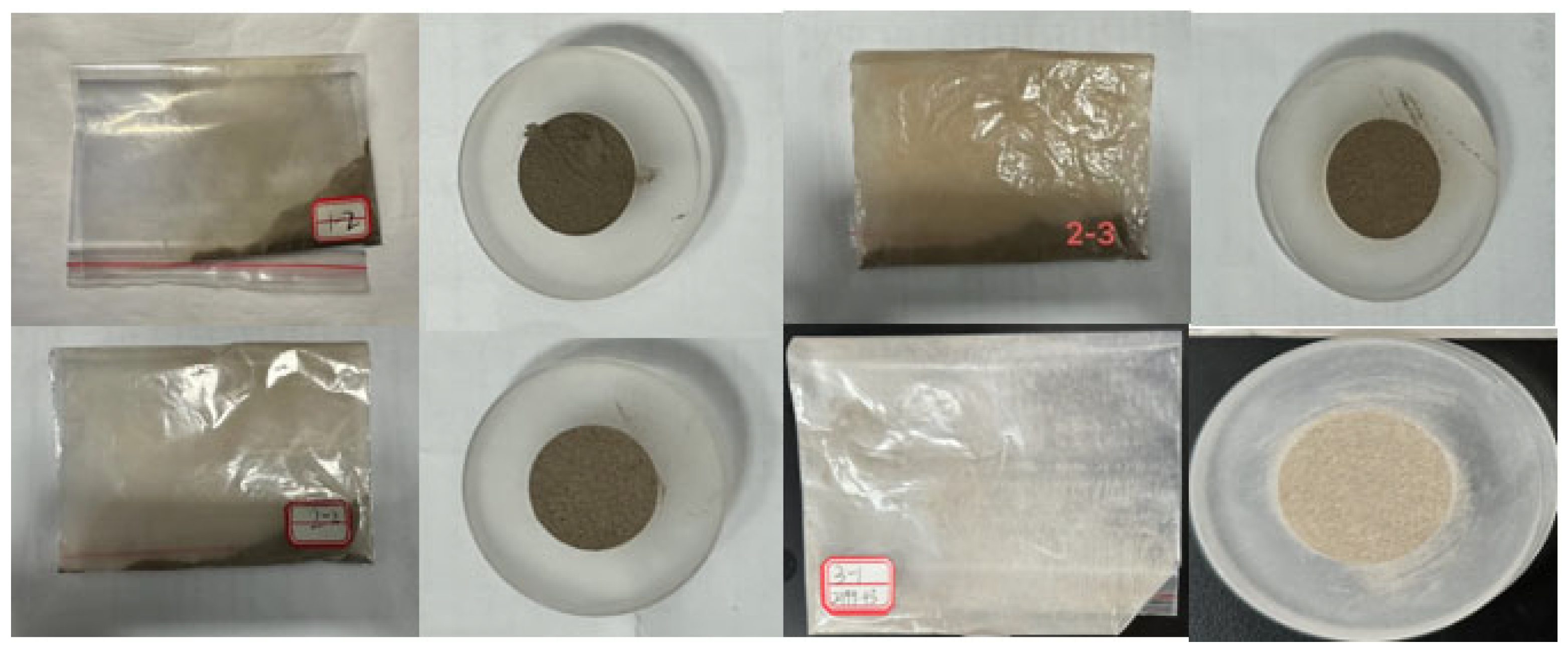
2.1. X-ray Diffraction Experiment

In 1912, Laue et al. [27] confirmed the periodic arrangement of atoms within tens to hundreds of picometers (pm) of each other in crystalline materials. This periodic arrangement of the atomic structure can become the “diffraction grating” for X-ray diffraction. X-rays have wave characteristics; specifically, they are electromagnetic waves with a wavelength of tens to hundreds of picometers that can diffract [28]. This experiment was the first milestone in X-ray diffraction.

A crystal is composed of cells of atoms arranged regularly, where the distance between these atoms arranged regularly is the same order of magnitude as the wavelength of the incident X-rays, and thus, this creates a diffraction grating. Therefore, when a beam of monochromatic X-rays is incident on a crystal, the X-rays scattered by different atoms interfere with each other, which results in strong X-ray diffraction in some special directions, with a spatial distribution in terms of the azimuth and intensity of the diffraction lines. This distribution is closely related to the crystal structure and the diffraction pattern produced by each crystal reflects the atomic distribution law inside the crystal. This is the basic principle of X-ray diffraction.

Phase analysis is the most commonly used aspect of X-ray diffraction in metals and includes both qualitative and quantitative analyses. The former compares the measured lattice plane spacing and diffraction intensity of the material with the diffraction data of the standard phase to determine the phase existing in the material. The latter determines the content of each phase in the material according to the intensity of the diffraction pattern. It has been widely used to study the relationship between the properties and content of each phase, the composition and distribution ratio of materials, and whether subsequent treatment procedures are reasonable. Samples are often not in a single phase; thus, people want to know the content of a certain phase. The understanding is that even an approximate result is better than no result at all. To illustrate the problem of quantitative analysis, we need to understand the information contained in the X-ray diffraction pattern. The information has three main aspects: the position of the diffraction peak, the intensity of the diffraction peak, and the shape of the diffraction peak. According to the three conditions of the diffraction peak, the quantitative features of the experimental sample are approximated.

The X-ray diffraction (XRD) samples were all low-permeability sandstones from Well X in the western South China Sea. Six groups of samples were selected from different depths of the reservoir for grinding and then filtered by 200-mesh and 300-mesh screens; six groups of powder samples were obtained, which were recorded as samples 1, 2, 3, 4, 5, and 6. The sample preparation process is shown in Figure 1.

The powder from the proper grinding of the 6 groups of whole-rock samples was filled into the groove of the sample rack such that the powder samples were evenly distributed in the groove and then pressed with a smooth slide. The excess powder outside the tank or above the sample rack was scraped away, and then the sample was flattened again so that the sample surface was at the same level as the edge of the sample rack surface, as required. The filling sample is shown in Figure 2.

In this experiment, phase qualitative analysis and phase quantitative analysis of the six groups of powder samples were completed using a multifunctional X-ray diffractometer (D8 ADVANCE, made in Germany) at Northwestern University (China). The D8 ADVANCE experimental equipment is shown in Figure 3. The D8 ADVANCE has excellent adaptability for typical X-ray powder diffraction (XRD), and with the D8 ADVANCE alone, we could measure all samples in this experiment. Not only this, but Bruker exclusively also offers a collimation guarantee based on the NIST standard sample corundum (ASTM UOP905-20 [29]). At present, no other powder diffractometer on the market exceeds the accuracy of the D8 ADVANCE in terms of peak position, strength, and resolution.

In the preparation and inspection stages before start-up, the prepared sample was inserted into the sample table of the diffractometer and the top and protective covers were closed. The faucet was turned on to make the cooling water flow. The X-ray tube window was checked to ensure that it was closed and the tube current tube voltmeter was in the minimum position. The main power supply and regulated power supply were switched on. In the start-up operation stage, the main power supply of the diffractometer was opened and the circulating water pump was started. After waiting for a few minutes, the computer X-ray diffractometer application software was opened; the tube voltage, tube current, and diffraction conditions and parameters were set to the required values, and the sample test was started. During the shutdown operation stage, after the measurement was completed, the system automatically saved the test data, the application software of the X-ray diffractometer was closed, and the sample was removed. After 15 min, the circulation pump, water source, general power supply of the diffractometer, and the circuit were turned off.

To retrieve the diffraction data of the analyzed sample, including the diffraction curve and d value, relative intensity, and diffraction peak width and other data, MDI Jade software was used to automatically determine the unique corresponding PDF card and retrieve the PDF card on the computer. Six groups of marine sandstones with low permeability were tested in this experiment. The 2^θ angle range of the experimental test was 4 ~ 90°, and the measurement speed was set to 2°/min.

The mineral quantitative analysis of the whole-rock XRD samples followed the international general Rietveld method, and the quantitative calculation of clay minerals followed the Standard Manual of Clay Mineral Analysis of the Geological Society of America (USGS). For the quantitative analysis of clay minerals, we needed to obtain X-ray diffraction patterns of the samples dried at 25 °C, dried at 60 °C after wetting with ethylene glycol and dried at 550 °C.

Figure 4 shows the X-ray diffraction results for the six groups of samples. The sequence number in the upper-left corner of Figure 4 is a map of each corresponding sample. By considering the position, intensity, and shape of the diffraction peaks of each sample, the whole-rock quantitative analysis was carried out.

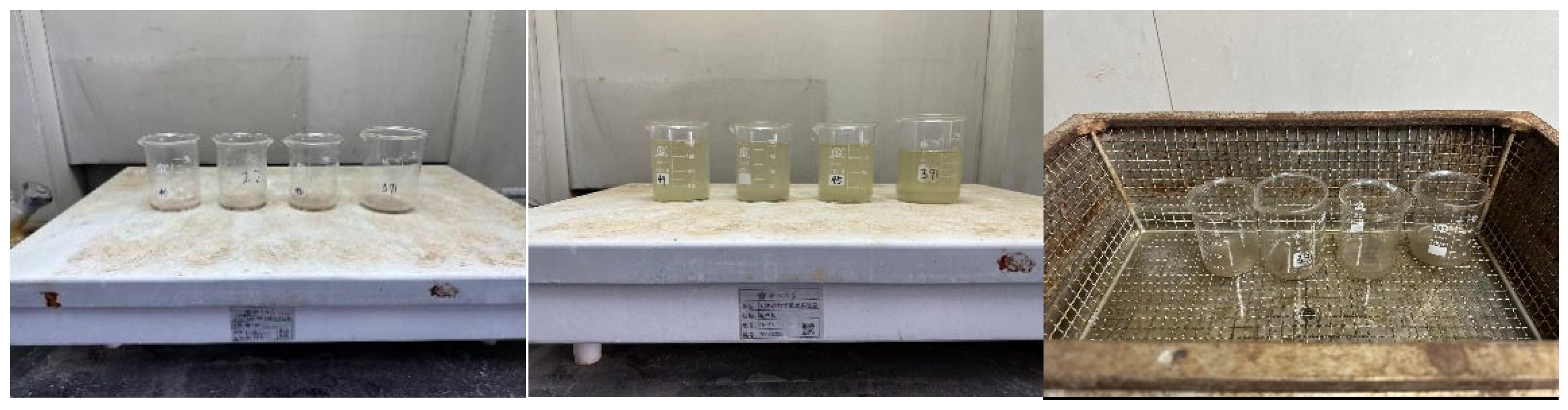
2.2. Laser Particle Size Analysis

The principle of laser particle size analysis is that, under laser irradiation, diffracted light generated by particles of different sizes falls in different positions, and the position information reflects the sizes of the particles. The diffracted light generated by particles of the same size falls into the same position, and the superimposed light intensity reflects the percentage of the particles. The wave front is limited by the aperture or particle, which is equivalent to the wavelength scale. Diffraction and scattering are generated by the spatial interference of the emission of each element wave as a source at the restricted wave front. The spatial (angular) distribution of the diffraction and scattered light energy is related to the wavelength of the light wave and scale of the aperture or particle.

With a laser as the light source, which has a certain wavelength of monochromatic light, the diffraction, and thus, the scattered light’s spatial (angular) energy distribution is only related to the particle size. For the diffraction of particle groups, the amount of each particle level determines the size of the light energy obtained at the corresponding specific angle, and the proportion of light energy at each specific angle in the total light energy should reflect the distribution abundance of each particle level. According to this idea, a mathematical and physical model can be established to characterize the abundance of particle sizes and the light energy obtained at each specific angle; then, an instrument can be developed to measure the light energy. Thus, the abundance ratio of the corresponding particle size can be derived by comparing the light energy measured at a specific angle with the total light energy. The particle size is obtained by measuring the intensity and position of the angular scattered light of the particle group.

The samples for the laser particle size analysis were all low-permeability sandstone from Well X in Weizhou. Four groups of samples were selected from the reservoir for percussion and were filtered through a 20-mesh screen. These were recorded as samples 1, 2, 3, and 4.

The four groups of samples were placed in different beakers, and 10 mL H₂O₂ with a concentration of 10% was added and heated on an electric heating plate. During the heating process, the wall of the burning cup was continuously washed with washing solution, and the paper foam disappeared. Another 10 mL of HCL at 10% concentration was added to the sample to remove the calcium gel substance contained in the sample. Water was added to the sample and stirred to neutralize and clean the calcium and chloride ions. After adding 10 mL of sodium hexametaphosphate (NaPO₃)6 solution with a concentration of 1 mol/L, the sample was fully dispersed. Finally, the sample was cleaned using a KQ-500E ultrasonic cleaner (made in Xi’an, China).

Figure 5 shows the removal of organic matter from the samples from left to right. Carbonate and calcium cement were removed from the sample, calcium and chloride ions were neutralized and cleaned, and the samples were dispersed.

Since 1981, the Mastersizer series of laser diffraction particle size analyzers have been successfully developed and improved by the Malvern Company in England using small-angle laser scattering technology. They are widely used in medicine, stone oil, water mud, oil paint, coatings, mineral product processing, powders, and military fields [30]. The Mastersizer 2000 (Mastersizer 2000 is a British company Malvern Instruments Limited, Malvern, UK) is a perfect combination of advanced laser diffraction technology and highly practical conventional particle characterization, and it has become the best choice for particle size analysis in laboratories around the world. The instrument provides fully automated measurements of powders, suspended substances, and emulsions, and it produces reliable measurements according to standardized procedures.

The Mastersize 2000 laser was added to the base of the main detector. The detection angle can be up to 135°, the detection limit of the particle size can be up to 20 nm, and large groups of particles at the nanometer or sub-micrometer level can be detected from the front and back detectors. To ensure that the light intensity signal of the small particles was large enough and to effectively reduce the noise of the large particle-scattering signal, the Mastersizer 2000 uses a specialized non-uniform cross-row fan detector for detection. The increase in sensor sensitivity is logarithmic, which maintains a high signal-to-noise ratio and avoids scattering signal loss. The last key factor is that the Mastersizer 2000 uses a high-energy light source to ensure that the detector can obtain a sufficiently strong scattering signal since it can efficiently reduce and even eliminate non-scattered light. The quality of the detector improved the precision of the measurement [30].

Using the Mastersize2000 laser particle size analyzer at Northwest University (China), the particle size analysis of 4 groups of samples was completed. Figure 6 shows the Mastersize2000 laser particle size analyzer at Northwest University, and the components of each part of the Mastersize2000 laser particle size analyzer are introduced.

System cleaning and instrument calibration (of the light) were performed. Before each sample experiment, a background measurement was carried out. After the background measurement was completed, the sample was poured into the sampler and measured when the shading reached the appropriate range. The sample measurement was completed after the measurement options had stated the results.

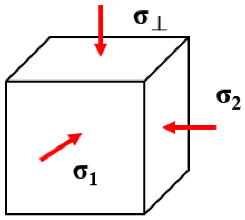
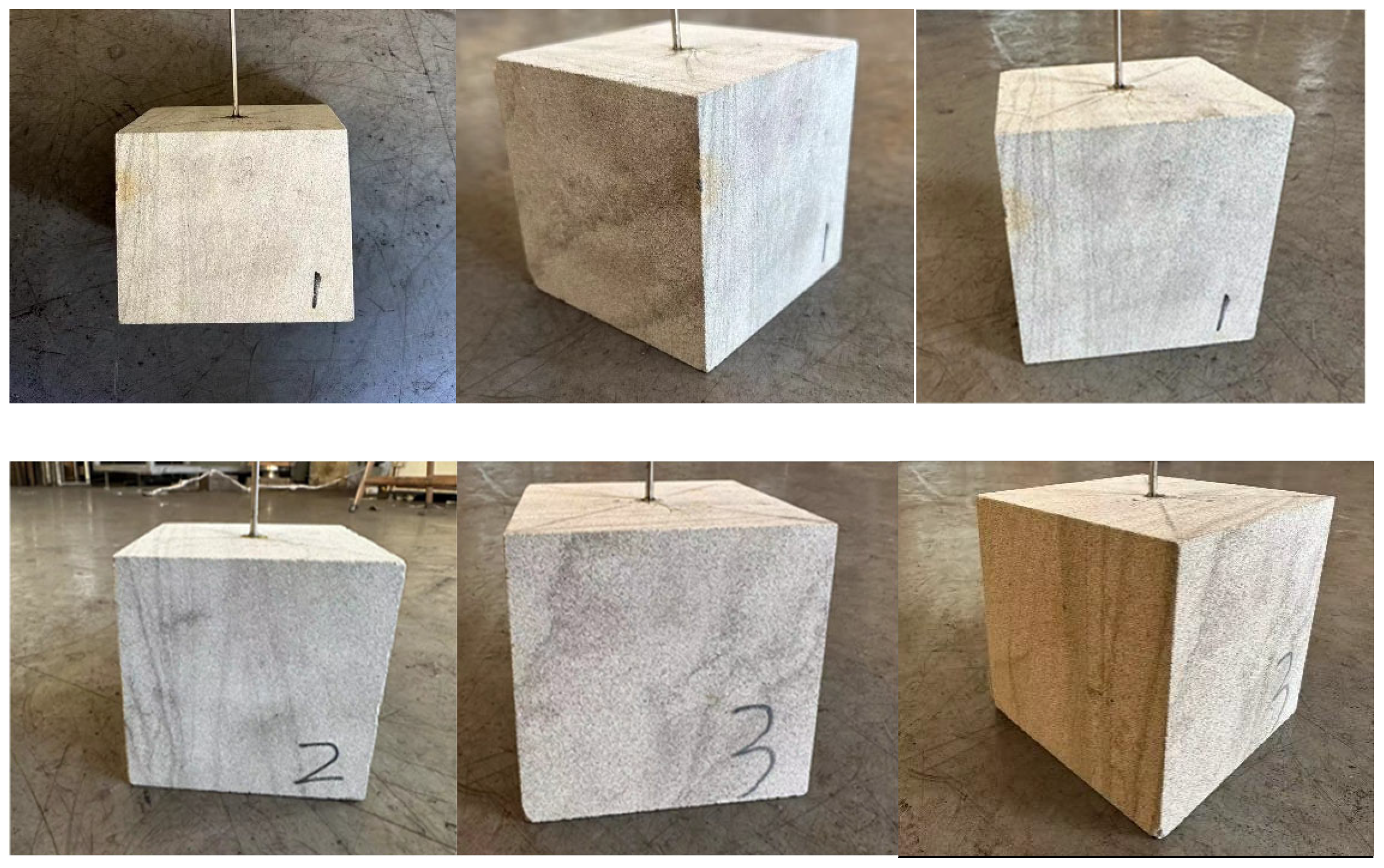
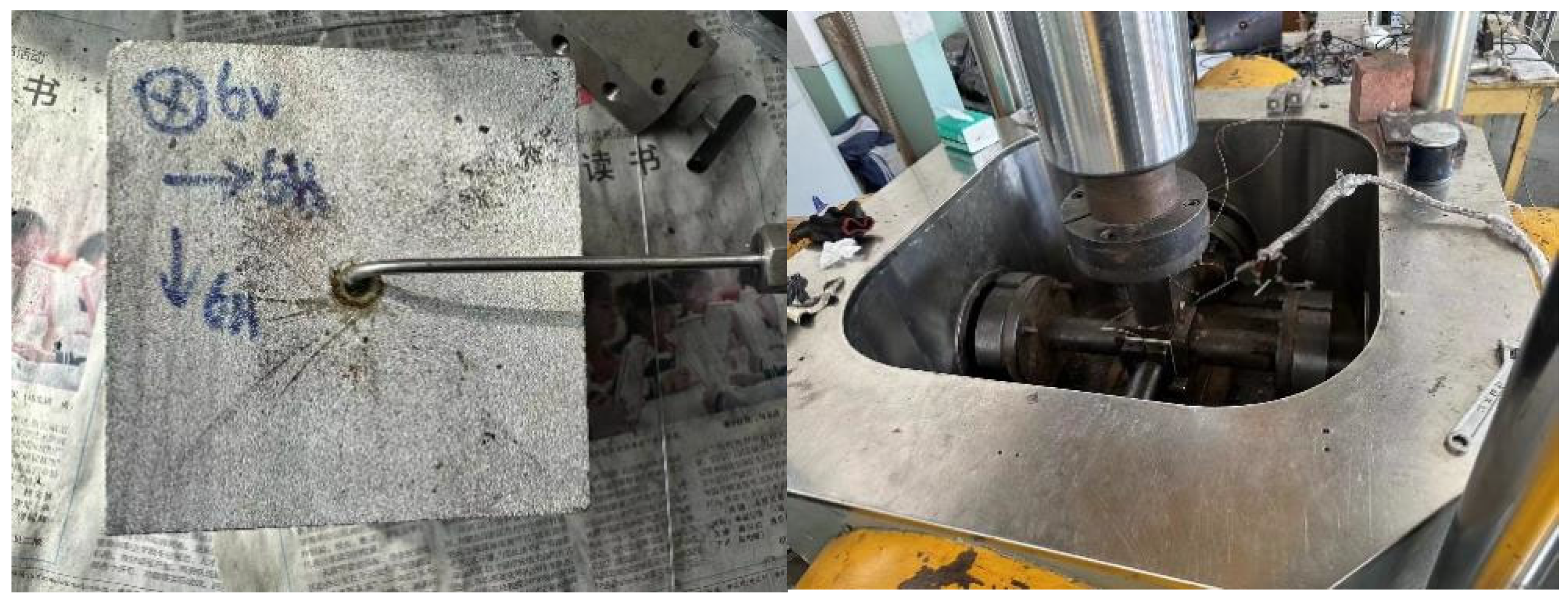
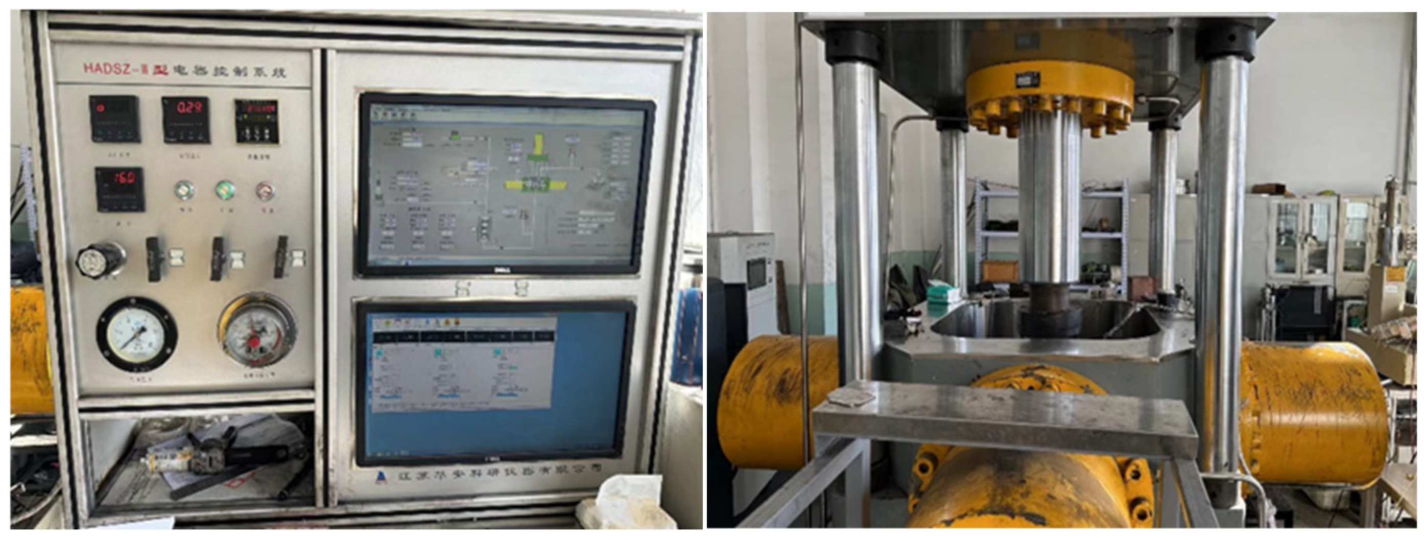
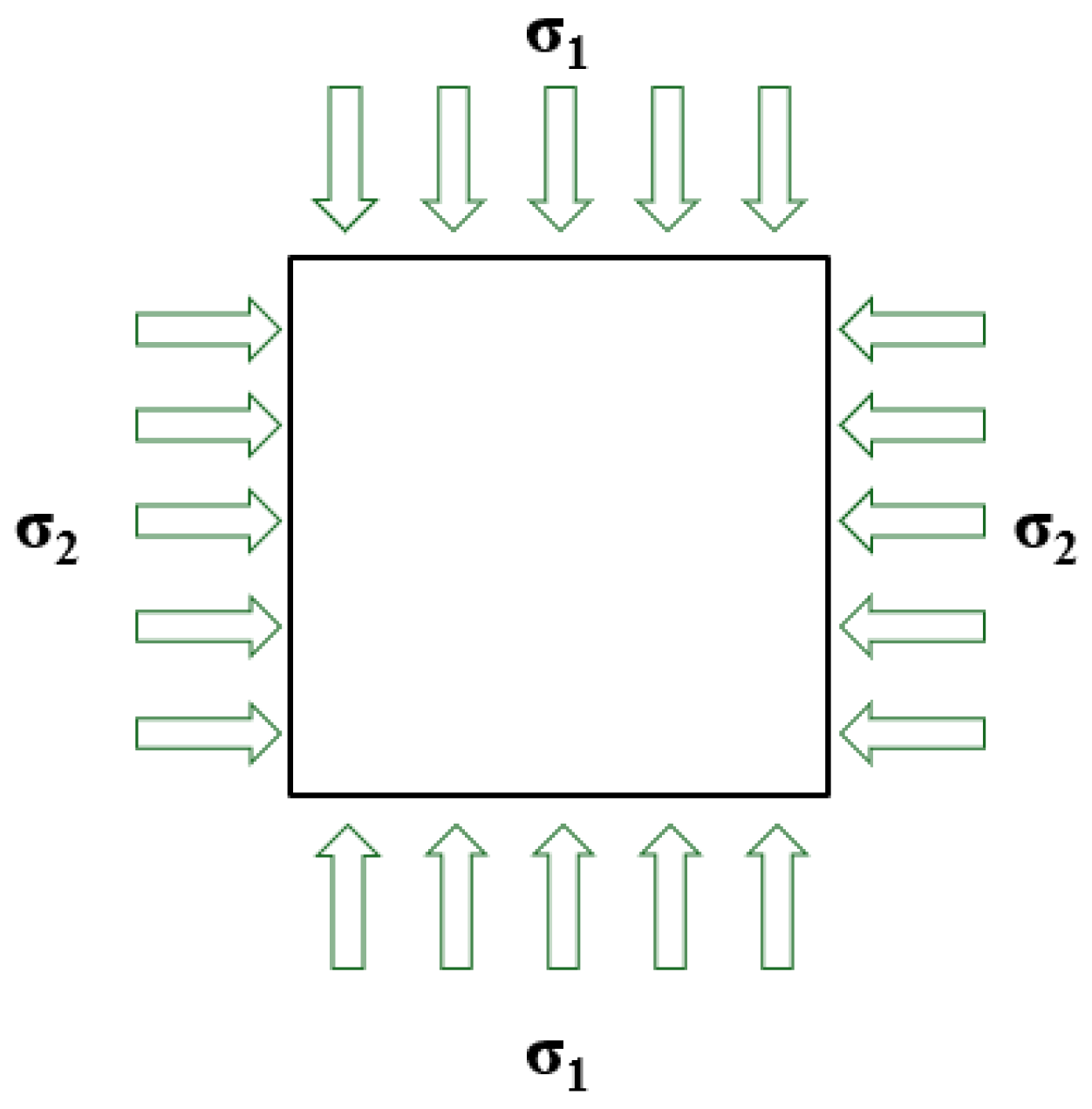
2.3. Physical Simulation Experiment of Water Injection Dilation in True Triaxial Rock Mechanics

A conventional triaxial experiment involves applying equal forces in two directions, that is, horizontal and vertical stresses, and there is no way to simulate the difference in horizontal stress. The stress conditions of conventional triaxial experiments are shown in Figure 7. The true triaxial experiment allows the three principal stresses to be unequal. The stress state under the complex geological and water injection conditions of the reservoir can be simulated more accurately.

$${\sigma }_{\perp }>{\sigma }_1={\sigma }_2,$$

(1)

where σ_⊥ is the vertical principal stress, σ₁ is the maximum horizontal principal stress, and σ₂ is the minimum horizontal principal stress (All variable symbols are shown in Abbreviations).

The true triaxial test can use either strain control or stress control, each of which has its own characteristics and advantages. The stress conditions of true triaxial experiments are shown in Figure 8. Under the strain control mode, the strain of the sample is uniform, the strain can be measured accurately, and the complex stress–strain path can be simulated. Under the stress control mode, the principal stress acts on the loading surface in the normal direction, and the stress distribution on each surface is uniform. This can achieve maximum strain without obvious boundary interference, which is easy to test according to the predetermined complex stress path.

$${\sigma }_{\perp }>{\sigma }_1>{\sigma }_2,$$

(2)

The sample preparation involved the “selection of stress surfaces” to apply a horizontal maximum principal stress, horizontal minimum principal stress, and vertical stress; “start water injection” was initiated after undertaking sample pump volume and pressure measurements.

In this experiment, according to the lithology, compressive strength, and porosity of the target reservoir, a similar rock was selected as the sample for a true triaxial rock mechanics physical simulation experiment of water injection dilation. The cube sample of 100 mm was made of rock, and the samples were marked as 1, 2, and 3. Holes of diameter 5 mm and depth of 55 mm were removed at the center of the top surface of the samples, and a metal pipe was inserted in the hole and sealed with glue. Samples 1, 2, and 3 are shown in Figure 9.

The top surface was judged according to the position of the water injection pipe, the vertical stress was applied to the top surface and the ground, and the directions of the horizontal maximum principal stress and horizontal minimum principal stress were selected. Glue was applied to the surface of the sample to connect the sample with the surface of the iron block. The displacement of the true triaxial mechanical machine pipe was controlled by the motor to control the pressure loaded by the machine on all sides of the sample. The pump pumped the liquid into the sample at a constant flow rate through the pipe. To ensure an appropriate liquid temperature, the liquid in the pump was electrically heated, and the peripheries of the pump and the pipe were wrapped with insulation. The sample and experimental equipment during water injection are shown in Figure 10.

This experiment used a true three-axis multifunction comprehensive experimental platform and the HADSZ-II electrical control system. The true three-axis multifunction comprehensive experimental platform and the HADSZ-II electrical control system are shown in Figure 11.

In the test system, two actuators were set in the same direction for synchronous alignment loading. This loading method required high servo control precision and could avoid the eccentricity problem during loading. Figure 12 is a schematic of double actuator loading under dual-axis conditions.

Pore pressure pretreatment was an experimental exploration in this study. It was considered that the rapid transient fluid injection was not conducive to the development of a reservoir fracture zone. Pressure-holding pretreatment was undertaken to fully inject the fluid into the rock mass to increase the dilation radius. This was exactly what happened. To better simulate a real formation water injection situation, hot water injection was chosen because the target layer was deep. The formation conditions were high temperature and high pressure.

Under the condition of true geostress, the two groups of experiments took constant displacement as the pump type, the fluid property was hot water (50 °C~80 °C), and the difference was whether to carry out pore pressure pretreatment. The test schedule is shown in

Table 1. Physical simulation test scheme for water injection dilation in true triaxial rock mechanics.

Simulation Experiment Type	Pore Pressure Pretreatment	Fluid Property	Injection Type of Capacity Dilation
Pressure-controlled water injection capacity dilation 1	Nothing	Hot water	Constant displacement
Pressure-controlled water injection capacity dilation 2	Nothing	Hot water	Constant displacement
Pressure-controlled water injection capacity dilation 3	Constant pressure for 3 h	Hot water	Constant displacement

.

3. Results

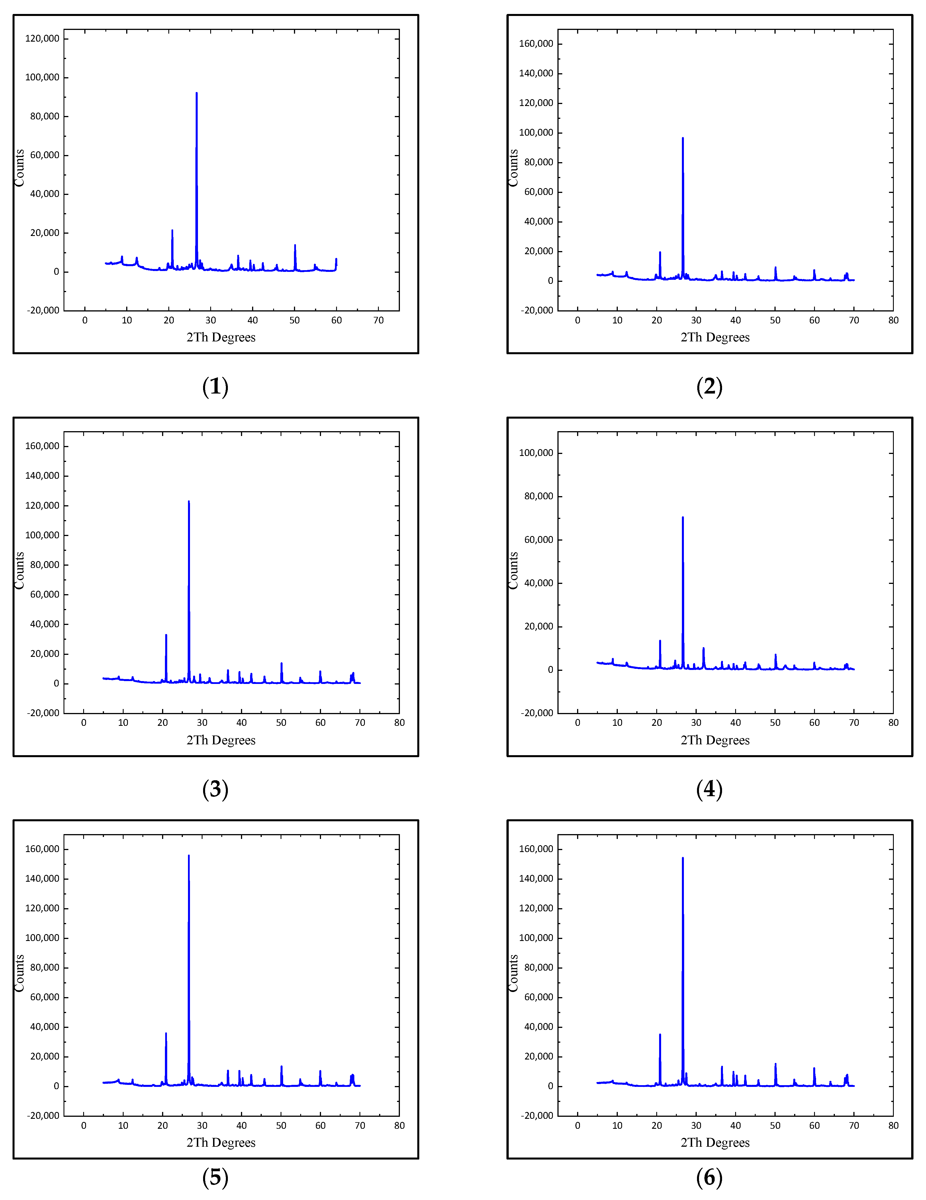
3.1. X-ray Diffraction Experiment

The brittleness of tight sandstone is one of the key factors in the exploration and development of tight oil and gas reservoirs. Taking the low-permeability sandstone of the offshore oilfield in the western South China Sea as an example, based on the geological data regarding the drilling core, rock thin sections, and geochemical characteristics, through the composition identification of sandstone under the microscope and the mineral content analysis by X-ray diffraction, it was found that the sandstone in the study area had a high quartz content. Therefore, a rock brittleness formula consistent with the regional background is obtained. The results show that low-permeability sandstone reservoirs in offshore oil fields in the western South China Sea have high brittleness and are suitable for water injection.

This could be obtained by interpreting the graphs for each sample in Figure 4. The proportion of clay in sample #1 was 10.15%, of which kaolinite accounted for 7.62% and illite accounted for 2.06%. The proportion of each clay mineral indicated that the hydration dilation effect of the sample was weak, which makes it more conducive to the implementation of water injection dilation technology.

Sample #2 was a reservoir sample from a depth of 2608.7 m. The main components of sample #2 were quartz, muscovite, kaolinite, and albitite, with quartz accounting for 42.34% and muscovite accounting for 23.43%. Sample #3 was a reservoir sample from a depth of 3176.73 m. The main mineral components of sample #3 were quartz, muscovite, kaolinite, and albitite, of which 61.69% was quartz and 12.82% was muscovite. Sample #4 was a reservoir sample from a depth of 3176.73 m. The main minerals in sample #4 were quartz, siderite, muscovite, and kaolinite, of which quartz accounted for 47.11% and siderite accounted for 20.76%. Sample #5 was a reservoir sample from a depth of 2199.43 m. The main minerals in sample #5 were quartz, muscovite, kaolinite, and chromium–potassium ore, of which quartz accounted for 62.88% and muscovite accounted for 16.17%. Sample #6 was a reservoir sample from a depth of 2200.1 m. The main minerals in sample #6 were quartz, muscovite, phosphorite, and kaolinite, of which quartz accounted for 70.85%, and muscovite accounted for 20.76%.

According to the XRD results of the six groups of samples with different reservoir depths, the non-clay minerals from the study area were mainly quartz and muscovite, and the content of non-clay minerals was more than 80%. The quartz particles were mostly angular, strongly hydrophilic, and had high dilatation potential. The main clay mineral in the study area was kaolinite; the content of clay minerals was less than 18%, and the hydration dilation was weak.

Figure 13 and

Table 2. Mineral content of samples.

Mineral Composition and Content/%		Sample 1	Sample 2	Sample 3	Sample 4	Sample 5	Sample 6
Non-clay minerals	Quartz	54.48	42.34	61.69	47.11	62.88	70.85
	Muscovite 2M1	20.28	23.43	12.82	12.40	16.17	12.70
	Gismondine	12.53
	Albite	1.25	8.79	5.95	3.65
	Sanidine	0.76	1.88
	Siderite			4.65	20.76
	Orthoclase	0.55	2.96
	Co-olivine		1.56
	Berlinite		0.15			4.63	5.6
	Lopezite			2.81	3.00	5.35	1.72
	Cuprite syn			0.11	1.32
	Anorthoclase					0.2	1.69
	Total	89.85	81.11	88.03	88.24	89.23	92.56
Clay minerals	Kaolinite	7.62	10.87	9.03	8.16	6.67	4.53
	Illite	2.06
	Glauconite	0.47	8.02	2.46	3.14	4.04	2.79
	Nontronite			0.48	0.46	0.06	0.11
	Total	10.15	18.89	11.97	11.76	10.77	7.43

show six column charts for the quantitative analysis of the whole-rock minerals of samples #1~#6, which show that the major mineral component of the six groups of samples was quartz, where the quartz particles were mostly angular, strongly hydrophilic, and had a high potential for dilatancy strength.

A mineral brittleness study of tight sandstone was undertaken to characterize the fracture development ability and late artificial fracturing potential of tight sandstone according to the content of brittle minerals. Because the tight sandstone in the Longmenshan foreland basin is rich in rock debris, the content of brittle minerals was studied and tested. First, the approximate composition and mineral content (clay minerals, quartz, and feldspar) were estimated by observing petrological thin slices under a transmittion light microscope [31]. In the study of tight sandstone, the more quartz content there is, the lower the brittle mineral content will be. The above data show that quartz was the mineral with the largest proportion in the mineral compositions of samples #1~6, all of which contained more than 40% quartz. Therefore, the percentage of quartz in the total amount of quartz and clay minerals could be used to calculate the brittleness of the rock in the sample [32]. The formula for calculating the mineral brittleness index of tight sandstone is shown in Equation (3):

$$B={\displaystyle \frac{{\sigma }_Q}{{\sigma }_Q+{\sigma }_{C\mathrm{m}}}},$$

(3)

where σ_Q is the proportion of quartz in the sample, %; σ_Cm is the proportion of clay mineral in the sample, %; and B is the sample brittleness index, -.

The total content of brittle minerals in the tight sandstone was high, the brittleness was high, and the development of natural fractures was easy, which was conducive to artificial fracturing and exploitation of tight gas in the later stage [33]. According to the experimental results, samples #1–#6 had brittleness values of about 0.84, 0.69, 0.84, 0.80, 0.85, and 0.91, respectively. Brittleness analysis of the six groups of samples showed that brittleness was above 0.65, and the average brittleness was 0.82. The brittleness indices of the six groups of samples are shown in Figure 14.

The results of the X-ray diffraction experiments and brittleness index calculations show that the higher the total content of brittle minerals in tight sandstone, the higher the brittleness, the easier the development of natural fractures, and the more conducive it is to waterflood dilation development.

3.2. Laser Particle Size Analysis Results

Particle size refers to the absolute size of clastic particles, and is the most important structural characteristic. The study of sedimentary rock grain size and grain size distribution characteristics uses methods collectively referred to as particle size analysis. Grain size analysis can distinguish formation hydrodynamic conditions and the sedimentary environment. For sedimentary rocks in different sedimentary environments, the particle sizes are different due to differences in hydrodynamic conditions. Moreover, the particle size of sedimentary rock has a strong control effect on the pore structure characteristics of the rock. It is generally believed that the finer the particle size of the rock, the worse is the pore structure performance. Therefore, grain size analysis data are very important for the evaluation of offshore low-permeability sandstone reservoirs [34].

In the laser particle size analysis experiment, the four groups of samples were from a 3176.73 m deep reservoir segment. The particle size distribution of sample #1 was 2.286 μm for d(0.1), 19.672 μm for d(0.5), and 113.352 μm for d(0.9), and the average volume particle size was 41.225 μm. According to the particle size grade, sample #1 was fine silt.

The particle size distribution of sample #2 was 4.020 μm for d(0.1), 61.561 μm for d(0.5), and 304.601 μm for d(0.9), and the average particle size was 109.130 μm. According to the particle size grade, sample #2 was mainly coarse silt and fine sand.

The particle size distribution of sample #3 was 3.674 μm for d(0.1), 45.654 μm for d(0.5), and 168.362 μm for d(0.9), and the average particle size was 72.382 μm. According to particle size grade, sample #3 was mainly coarse silt.

The particle size distribution of sample #4 was 2.839 μm for d(0.1), 32.518 μm for d(0.5), and 129.919 μm for d(0.9), and the average particle size was 51.528 μm. According to the particle size grade, sample #4 was mainly coarse silt.

In Figure 15, the four diagrams are the particle size and cumulative particle size distribution diagrams of samples #1~#4 according to the labels in the upper-left corner of each diagram. The four diagrams show that the four groups of samples were mainly coarse silt, and the particle size distributions were relatively concentrated.

The formulas for the particle size parameters can be roughly divided into two categories: formulas that use the graphical method and formulas that use the moment value method. The graphical method is mainly cumulative. The method for calculating the particle diameter at a specific cumulative percentage on the curve is simple and can be compared with the cumulative frequency curve. Compared with the moment value method, the particle size distribution characteristics can be displayed more intuitively. The moment value method does not require cumulative frequency curves and directly analyzes all grain sizes. The aggregate calculation of the occupied percentage can fully reflect the characteristics of the sediment particle size distribution, but the calculation process is more complicated [35].

The development of the graphical method can be roughly divided into three stages: Trask’s quartile method [36], Inman’s graphical method [37], and Folk et al.’s comprehensive graphical method [38]. The current national standard (GB/T 12763.8 [39]) uses the Folk–Ward formula to calculate particle size parameters. Trask believed that the sediment could be characterized by the median particle size; therefore, the Trask formula uses the median particle size instead of the average particle size. Later, Inman used the particle size values of 16% and 84% of the cumulative frequency curve to calculate the average particle size, which allows for covering a wider range of particle size distributions. Based on Inman’s formula, the Folk–Ward method adds a particle size of 50% of the cumulative frequency curve to the calculation formula of the average particle size, so that not only the coverage of the particle size but also the weight of the median particle size are considered [32].

The sorting coefficient formula proposed by Trask can judge the particle size dispersion degree of a sample by the ratio of the corresponding particle sizes at 75% and 25% of the cumulative distribution curve, and its advantage is that the influence of the unit is eliminated by the ratio (Trask P D. 1930 [36]). Inman and Folk–Ward calculated the separation coefficient using the difference in the particle size corresponding to different percentages of the cumulative curve. The formula given by Inman used ϕ₈₄ and ϕ₁₆ to calculate the sorting coefficient (Inman D L., 1952 [37]), and the sorting coefficient formula proposed by Folk–Ward further expanded the range of particle size distribution involved in the calculation, where they combined the proportions of the two intervals (ϕ₈₄ − ϕ₁₆, ϕ₉₅ − ϕ₅) with a normal distribution characteristic value to have a wider applicability.

The evolutions of the skewness and kurtosis formulas are similar, and the formulas are modified by changing the percentile of the cumulative frequency curve. The skewness formula given by Trask only uses the particle size of the quartile (i.e., 25%, 50%, and 75%), while the kurtosis formula uses the particle size of the first and last quartiles (25% and 75%) and tenths (10% and 90%). Inman’s modified formula makes the coverage of skewness and kurtosis more comprehensive than Trask’s formula. Folk–Ward’s modification based on Inman enables the calculation of skewness to better measure the overall skewness of a sample and further adds the dispersion between different percentiles to the calculation of kurtosis. It has the effect of a visualized relationship between the kurtosis formula and the particle size distribution curve (Folk R L, et al. 1957 [38]).

To quantitatively calculate the uniformity or character of the particle size composition, the sorting grade parameter was introduced. Folk and Ward proposed using the size of the normal distribution standard deviation σ1 to classify the gradation of particle sorting. The standard deviation parameter consists mainly of the main range of ϕ₁₆ to ϕ₈₄ on the cumulative distribution curve based on the diameter, with features including the head (ϕ₅) and the tail (ϕ₉₅) of the curve. The quantitative analysis formula for the rock particle size is

$$\sigma ={\displaystyle \frac{{\varphi }_{84}-{\varphi }_{16}}{4}}+{\displaystyle \frac{{\varphi }_{95}-{\varphi }_5}{6.6}},$$

(4)

where σ is the standard deviation, ϕ₅ is the 5% volume fraction, μm, ϕ₁₆ is the 16% volume fraction, μm; ϕ₈₄ is the 84% volume fraction, μm, and ϕ₉₅ is the 95% volume fraction, μm.

According to the size of the normal distribution standard deviation proposed by Folk and Ward, the classification grade of rocks with a standard deviation of less than 0.35 is excellent, a standard deviation of 0.35~0.71 is good, a standard deviation of 0.71~1.00 is medium, a standard deviation from 1.00 to 4.00 is poor, and a standard deviation greater than 4.00 is extremely poor. Samples’ sorting grades are shown the

Table 3. Samples’ sorting grades.

Serial Number	ϕ5 (mm)	ϕ16 (mm)	ϕ84 (mm)	ϕ95 (mm)	σ1	Sorting Grade
1	0.00126	0.00288	0.07943	0.13804	0.04	Excellent
2	0.00191	0.00661	0.18197	0.41687	0.11	Excellent
3	0.00166	0.00501	0.11701	0.23988	0.06	Excellent
4	0.00145	0.00380	0.09120	0.18897	0.05	Excellent

.

3.3. Physical Simulation Experiment of Water Injection Dilation in True Triaxial Rock Mechanics

To simulate the rock physical properties of the target reservoir, a sandstone outcrop was used in this experiment. The core had a porosity of 7.06% and compressive strength of 50.23 MPa, which were close to the physical properties of the target reservoir core. The core was cut into a cube sample of 100 mm × 100 mm × 100 mm and polished to ensure that the opposite sides of the cube were parallel and the adjacent sides were vertical.

The real formation pressure gradient of the target reservoir was obtained from field data and laboratory experiments. The in situ stress was calculated according to the target reservoir depth and in situ stress gradient. The effective triaxial stress was 19 MPa for the vertical stress (σ_⊥1), 14 MPa for the maximum horizontal principal stress (σ_H), and 8 MPa for the minimum horizontal principal stress (σ_h). The pressure application scheme for sample 1 is shown in Figure 16.

Sample 1 was pretreated with a 70 °C aqueous solution without constant pressure and injected at a constant flow rate (0.2 mL/min or 1 mL/min). When the pump pressure of the sample reached 16.3 MPa, the pump pressure could not continue to rise. Combined with the field data, it was considered that the rock reached the fracture pressure. Under the condition of true triaxial rock mechanics, the fracture pressure of the target reservoir rock was 16.3 MPa. To realize the water injection dilation technology, the maximum pressure of samples 1 and 2 should not exceed 16.3 MPa after water injection. Because of the differences between the samples, it was safe to stop pumping liquid after the pump pressure reached 15.8 MPa after water injection. According to the site construction conditions and similarity criteria, the liquid was pumped into the sample at a constant rate of 1 mL/min.

The first set of experiments in this study were the rupture pressure exploration experiments. The rupture pressure of the experimental sample was obtained from the first set of pump pressure curves. When the injection pressure of sample 1 did not increase with the increase in injected water, the rock was considered to be broken. The highest pressure was the rupture pressure, which was 16.3 MPa. In this study, 16.3 MPa was considered the rupture pressure of this group of samples.

Pore pressure pretreatment was a kind of experimental exploration in this study. Transient rapid fluid injection was not considered conducive to the development of reservoir fracture zones. The pressure-holding pretreatment was performed to fully inject the injected fluid into the rock mass to increase the expansion radius, which was the result we achieved. To better simulate the real formation of the water injection, hot water injection was selected because the target layer was deep. The formation conditions were high temperature and high pressure.

Sample 2 was pretreated with a 70 °C aqueous solution without constant pressure and was injected at a constant flow rate (1 mL/min); the specific water injection flow curve is shown in Figure 17b. When the pump pressure of the sample reached 15.8 MPa, the pump was stopped, as shown by the water injection pressure curve in Figure 17a. According to the experimental results, sample 1 reached the set pump pressure after pumping 81.39 mL of the liquid. The real-time liquid flow rate, real-time pump pressure curve, and cumulative liquid flow rate of sample 2 are shown in Figure 17a, b, and c, respectively. It can be seen from Figure 17 that the pump pressure increased slowly in the early stage of the water injection with a constant flow rate and increased when the water injection duration reached 3000 s. When the pump injection pressure reached 12 MPa, the pump pressure growth rate slightly decreased.

Sample 3 was pretreated with an aqueous solution and a 6.24 MPa constant pressure for three hours, and the specific water injection pressure curve is shown in Figure 18a; then, it was injected at a constant flow rate (1 mL/min), and the specific water injection flow curve is shown in Figure 18b. When the sample pump pressure reached 15.8 MPa, the pump was stopped. According to the experimental results, sample 3 reached the set pump pressure after pumping 76.51 mL of the liquid. The real-time liquid flow rate, real-time pump pressure curve, and cumulative liquid flow rate of sample 3 are shown in Figure 18a, b, and c, respectively. Figure 18 shows that the initial flow rate was fast when the pore pressure pretreatment was performed under the condition of constant pressure as water injection, and then gradually stabilized at 0 mL/min. After pore pressure pretreatment, the pump pressure increased quickly at a constant flow rate, and the initial pump pressure did not increase slowly.

4. Feasibility Analysis of Water Injection Dilation

The above experimental results show that it was very feasible to exploit the target reservoir by using water injection dilation technology and carry out a true triaxial rock mechanics water injection physical simulation test for the target reservoir. Under true triaxial geostress, physical simulation tests of water injection dilation of offshore sandstone were carried out under constant pressure, step pressure, constant flow, different fluid properties, and cyclic oscillation dilation conditions. Red pigment was added to the injected liquid, the test sample was opened after the test, and the dilation effect of the water injection was judged according to the red area of the test sample. The feasibility of using the water injection dilation technology for low-permeability sandstone at sea was judged by the fracture production around and away from the water injection wellbore of the test samples.

4.1. Surface Analysis of Samples

Before the water injection, the cubic samples 1, 2, and 3 were clearly found to be intact and without cracks. According to Figure 19, the after-injection samples 1, 2, and 3 in the physical simulation experiment of true triaxial rock mechanics have red areas of varying degrees. Since the experimental pumping pressure was controlled below the sample rupture pressure, it was proved that the all the three samples showed dilatation. The red permeable region of sample 2 was the smallest, and the red permeable region of sample 3 was the largest. It was concluded that it was easier to achieve water injection dilation with the constant pressure pretreatment sample.

Subsequently, the sample was knocked open, where Figure 20 shows that the crack was perpendicular to the direction of the horizontal minimum principal stress.

Figure 21 clearly shows that there was a red part in this section, which was divided into water injection dilation areas.

In addition, 1 cm cubes were removed from near the wellbore area (red area) and far from the wellbore area (normal area) for electron microscope scanning. According to the scanning results, evident cracks appeared near the wellbore area, while no cracks occurred far from the wellbore area. Combined with the red area of the sample, it was concluded that cracks were generated by the physical simulation test of the true triaxial rock mechanics waterflood dilation.

4.2. SEM Analysis of Samples

The red area can be clearly seen in Figure 21., which proves that the cubic sample displayed the dilatation phenomenon. Since the water injection pressure was less than the rock rupture pressure and the tensile dilatation belonged to the state of isotropic dilation of the rock, the existence of a crack zone could not be clearly observed with the naked eye, and the high-magnification technology of scanning electron microscopy was used to find the crack. A scanning electron microscope (SEM) is a kind of observation method that uses a transmission electron microscope and a light microscope.

It uses a very narrow, focused, high-energy electron beam to scan the sample, and through the interaction between the beam and the matter, various physical processes are excited, and the related information is collected, amplified, and re-imaged to achieve microscopic morphology characterization of the matter. New scanning electron microscopes have resolutions of 1 nm. The magnification can reach 300,000 times and is continuously adjustable. The depth of the field is large, the field of view is large, and the three-dimensional imaging effect is good. In addition, the scanning electron microscope and other analytical instruments can be combined to observe the microscopic morphology and analyze the composition of the micro-region of the material.

SEM analysis is mainly divided into eight steps: sample preparation, sample loading, vacuum preparation, software operation, observation and focusing, high-magnification observation, screenshot preservation, and sample unloading.

Sample preparation: ensure that the sample is dry, attach the sample to a conductive adhesive, and use a clean compressed gas to purge the sample surface. Sample preparation is shown the Figure 22.

Sample loading: the conductive adhesive containing the sample is placed on the sample table of the scanning electron microscope, and the height and position of the sample table are adjusted so that the sample is in the best observation position.

Vacuum preparation: close the sample chamber door and start vacuuming until the conditions required for using the SEM are reached.

Software operation: open the control software of the scanning electron microscope and apply the necessary settings, such as the acceleration voltage and working distance.

Observation and focusing: initially focus the sample at low magnification, and then adjust the brightness and contrast until a clear image is observed.

High-magnification observation: switch to high-magnification mode and further adjust the focal length and imaging parameters to obtain high-resolution images.

Screenshot saving: when the image has reached the best resolution, take a screenshot and save it to the specified storage media.

Sample unloading: after the observation, turn off the acceleration voltage, release the vacuum in the sample chamber, open the sample chamber door, and take out the sample.

Figure 23 shows the electron microscope scanning results, where it is obvious that there is a fracture zone near the wellbore (red area). The scale of each picture in Figure 23 is shown in the lower-right corner. The scales of the pictures indicate that the fractures generated near the wellbore could exceed the mm level.

According to Figure 24, there were no fracture zones in the samples collected far from the wellbore (no red area). By comparing Figure 23 and Figure 24, the fracture zone in Figure 23 was generated after water injection dilation, which proved that the low-permeability sandstone is suitable for water injection dilation technology.

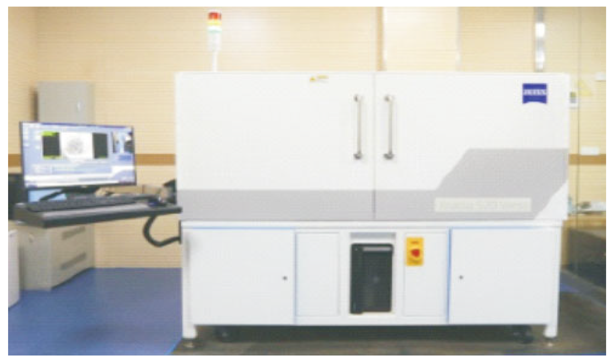
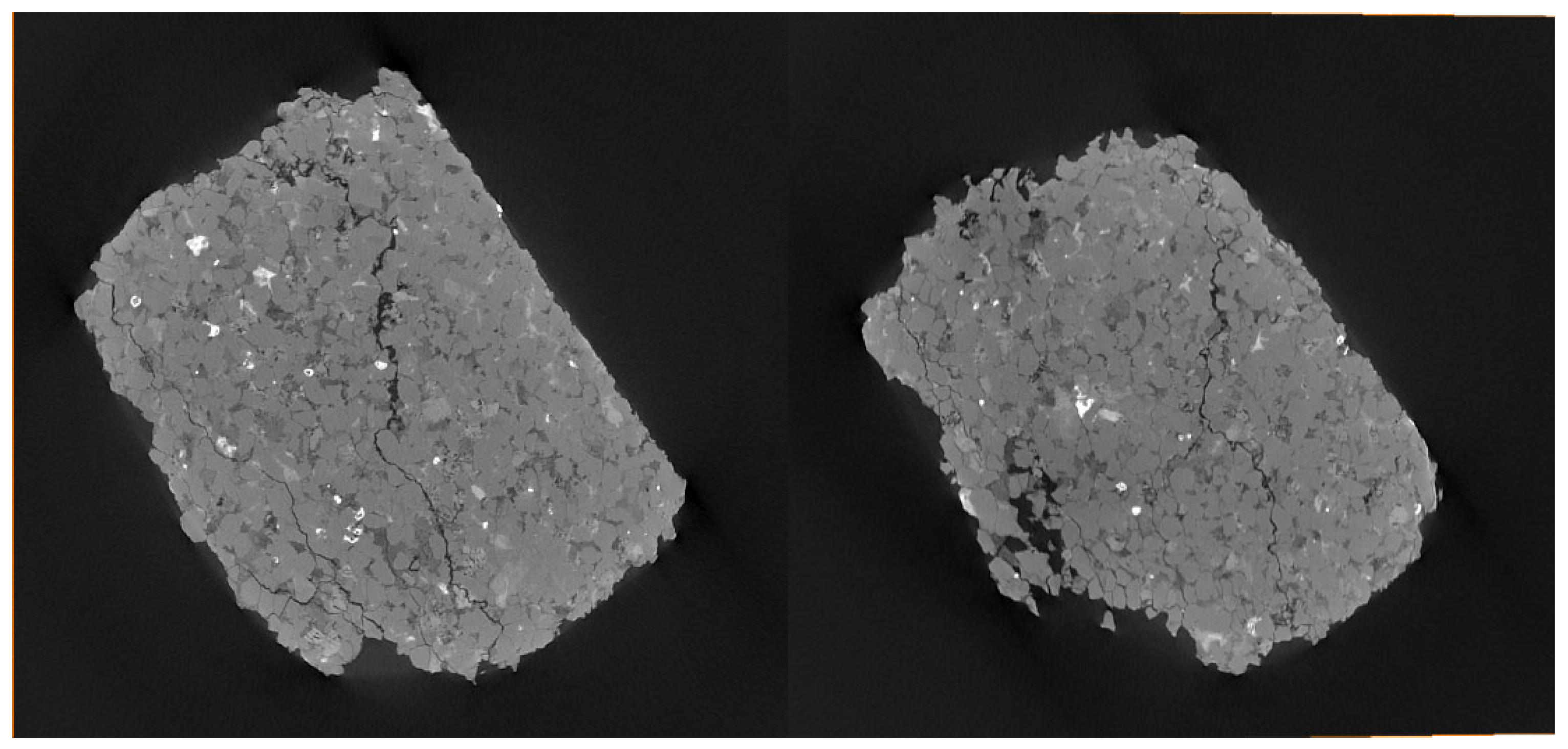
4.3. Three-Dimensional X-ray Microscope Analysis of Samples

An X-ray three-dimensional microscope produces X-ray imaging at the microscopic level; that is, the image magnification of the instrument can be used to observe and study microscopic structures invisible to the naked eye. The contrast principle of X-ray imaging, the structure of the equipment, and the main components (such as X-ray sources and detectors) are mainly from the imaging of macroscopic objects. There are similarities between macroscopic imaging and microscopic imaging, such as the contrast principle and the main components of the equipment, but there are also differences. Because an X-ray microscope is used to observe microstructures that cannot be resolved by the naked eye, there are significant differences in the instrument structure and requirements, such as requiring a small light source size and high intensity to enlarge the image and provide high resolution.

The imaging principle of an X-ray three-dimensional microscope is basically the same as that of an optical microscope, which follows the principle of geometric optics, and its key components are the optical components for imaging and amplification, which are lenses in optical microscopy. Because the wavelengths of X-rays are very short, the refractive index at the interface of the glass and the general material is close to 1, and thus, the imaging amplification element cannot use a glass lens, and a band plate is generally used instead.

The Xradia 520 Versa from Carl Zeiss (Carl Zeiss originated in Oberkochen, Germany) at the Northwestern University was selected for this experiment. The device has a spatial resolution of up to 0.7 μm and a minimum achievable voxel size of 70 nm. The Xradia 520 Versa X-ray microscope is shown the Figure 25.

The pore structure of the sample can be clearly seen in the figure below. A fracture zone was found in the regular pore structure, which was generated near the pipe after the water dilation. For the same sample, the 3D X-ray scanning results of the samples collected far from the wellbore showed no evident fracture zone. Samples collected far from the wellbore is shown the Figure 26.

5. Conclusions

This study mainly focused on an offshore low-permeability reservoir through X-ray diffraction, laser particle size, and scanning electron microscope experiments to analyze and judge whether offshore low-permeability sandstone was suitable for water injection dilation technology.

(1)

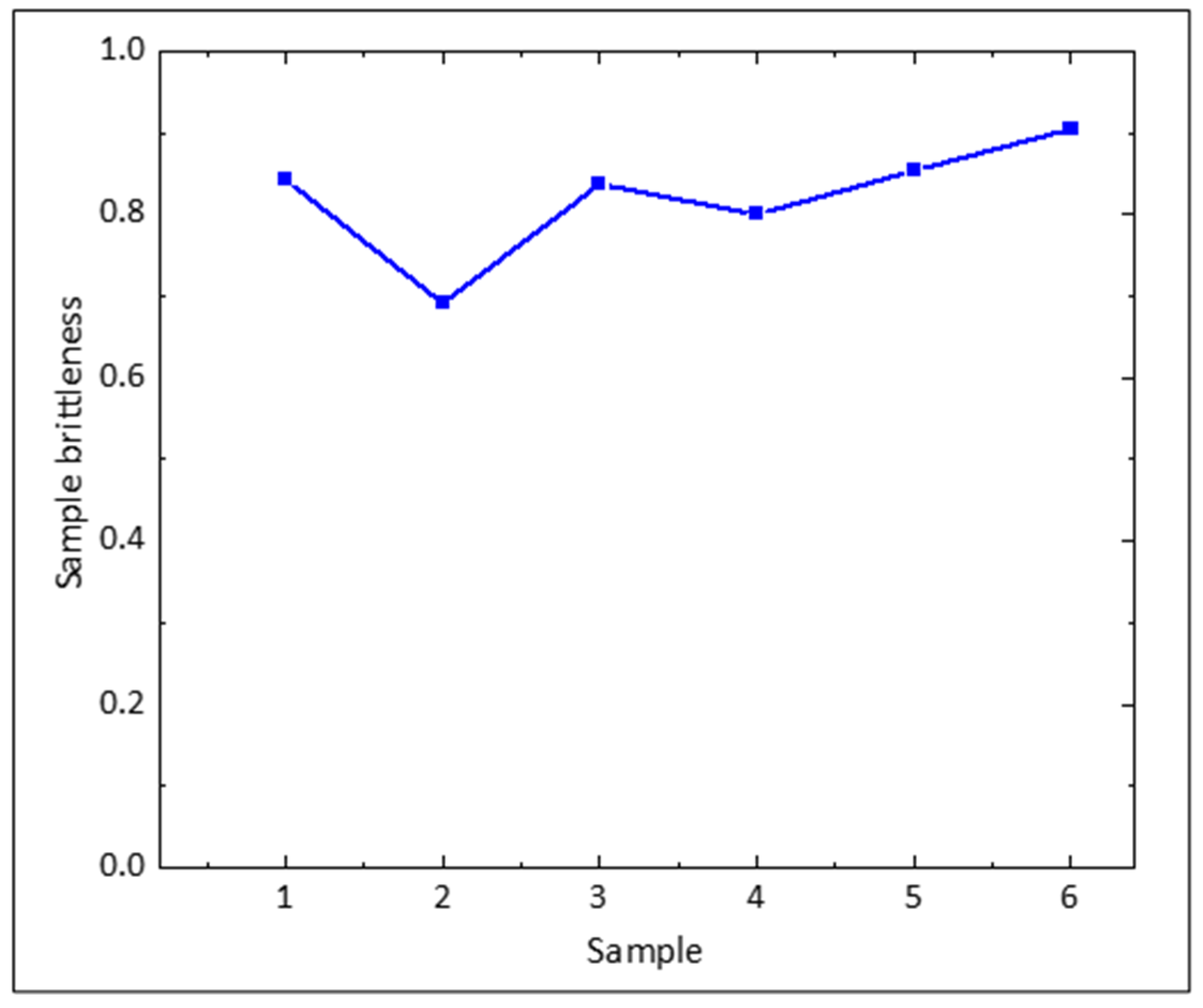
The XRD experiments showed that the minerals in the target reservoir section were mainly quartz and muscovite, and the content was more than 80%. The quartz particles were mostly angular, strongly hydrophilic, and had high dilatation potential. The brittleness analysis of the six groups of samples showed that their brittleness was above 0.65, and the average brittleness was 0.82. Previous scholars have found that the higher the content of brittle minerals in tight sandstone, the higher the brittleness, the easier it is to form fracture zones, and the more favorable the formation of complex fracture zones in water injection dilation development.

(2)

The laser particle size analysis experiment showed that the particle size of the target reservoir was mainly between 10 μm and 100 μm, and it could be classified as coarse silt according to the particle size division. According to Folk and Ward, the normal distribution standard deviation was used to judge the sorting grade of the target reservoir, which was found to be suitable for the development of an offshore target reservoir by the water injection dilation technology.

(3)

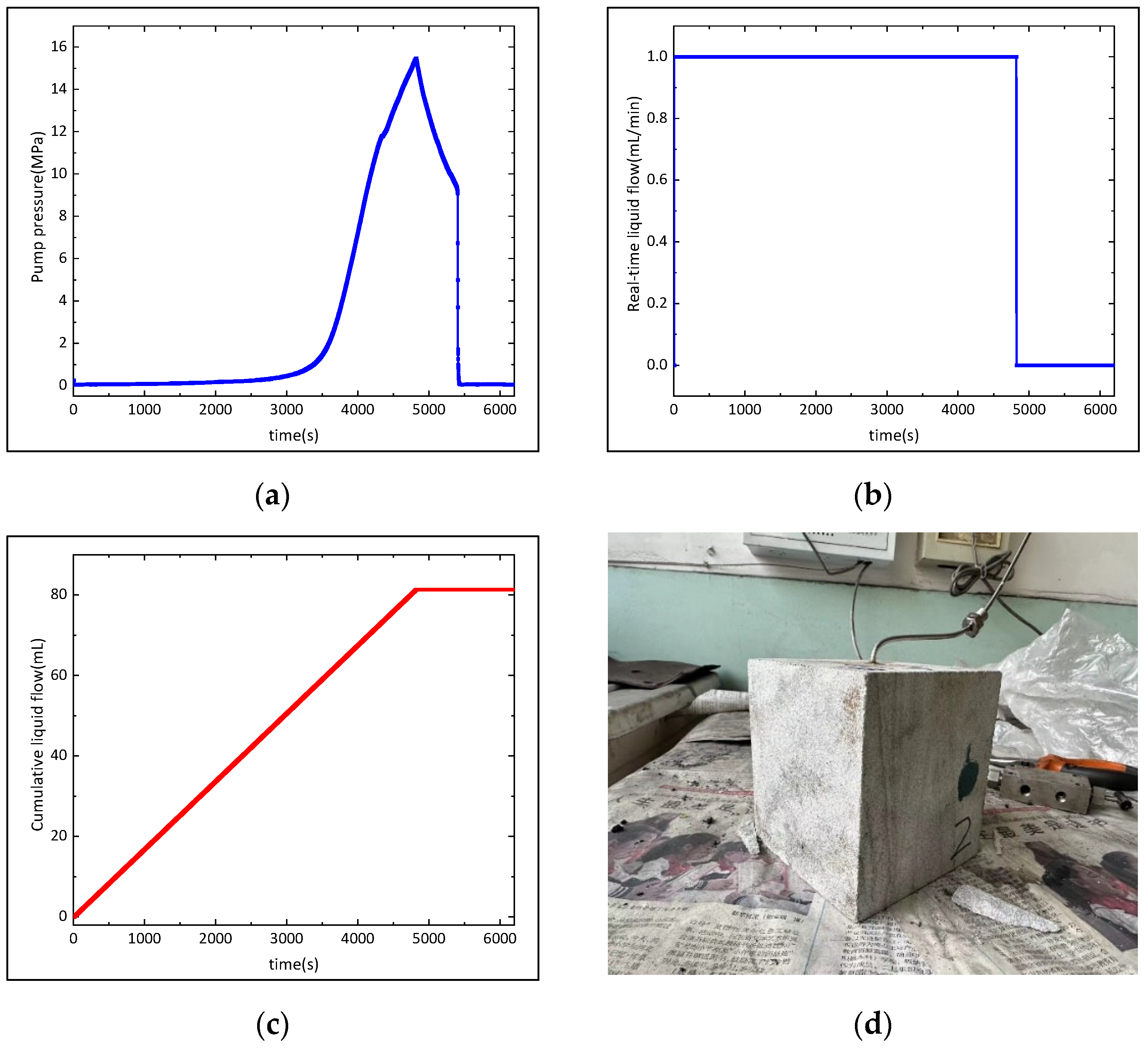
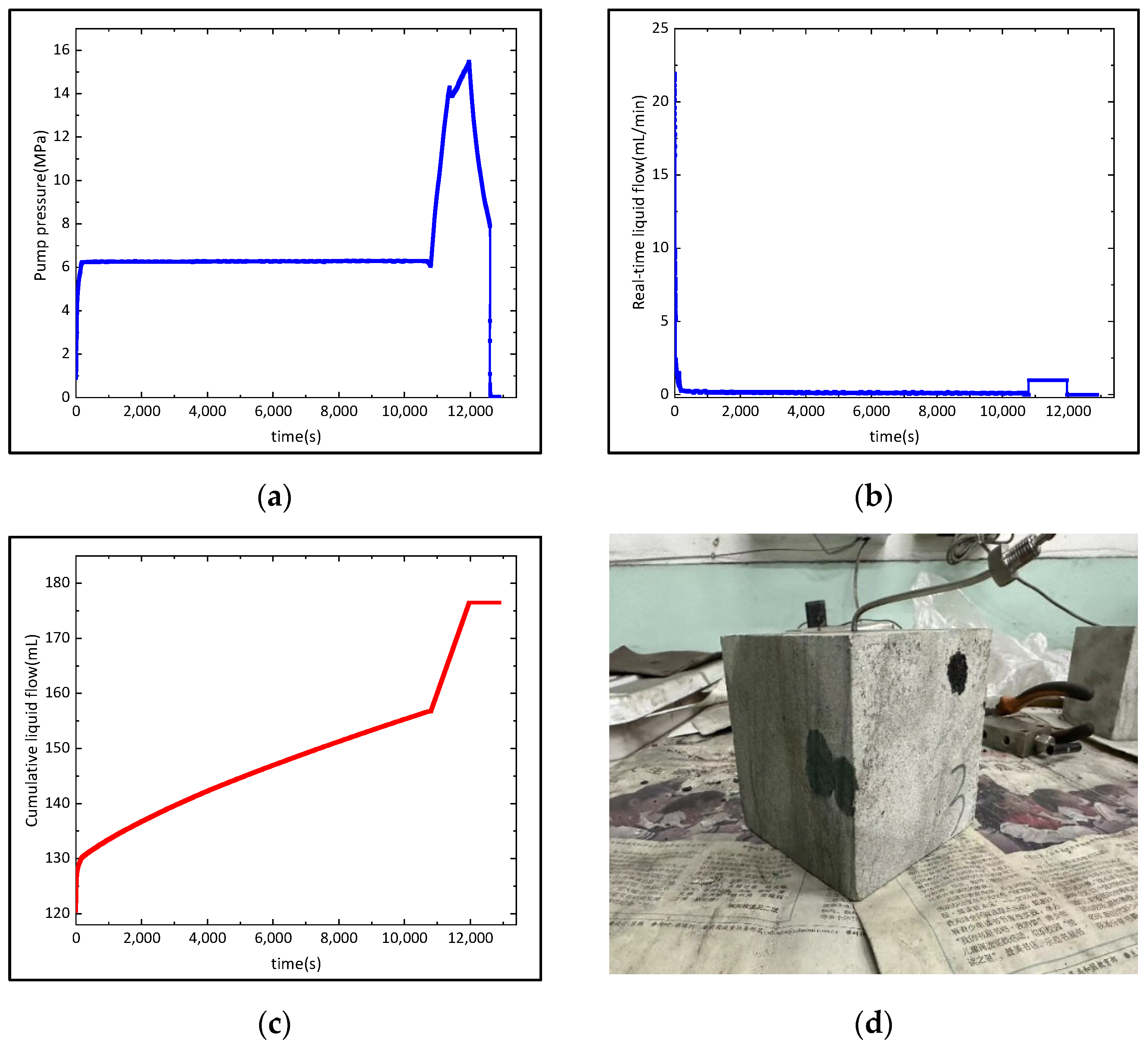
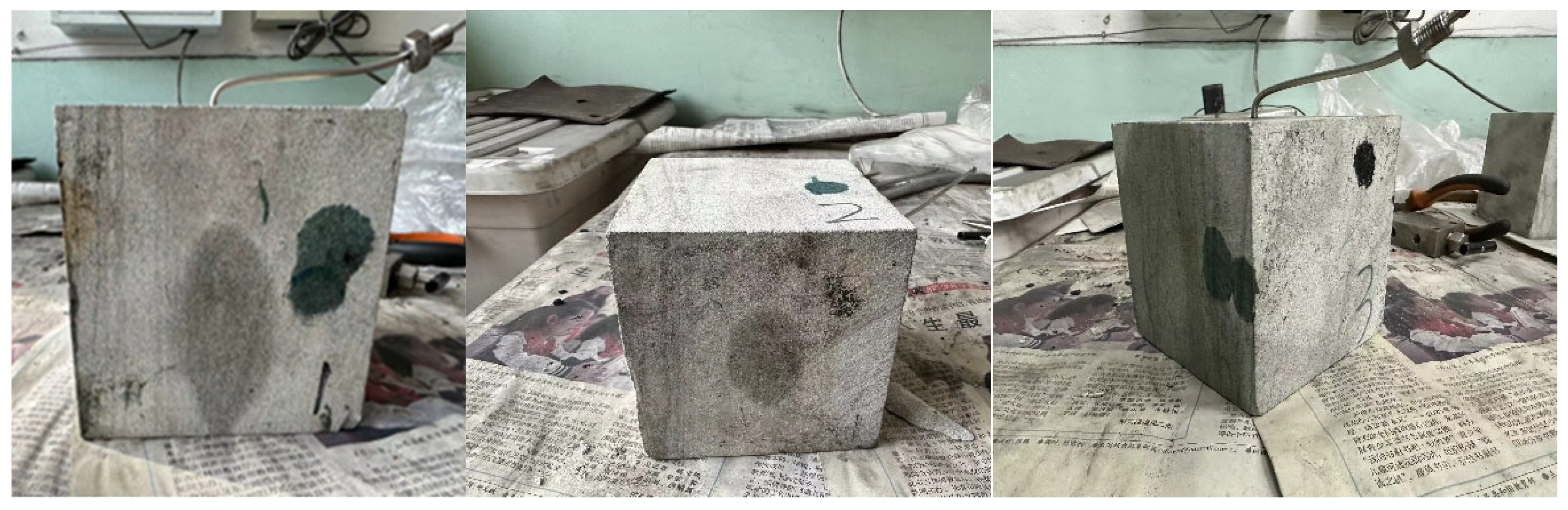
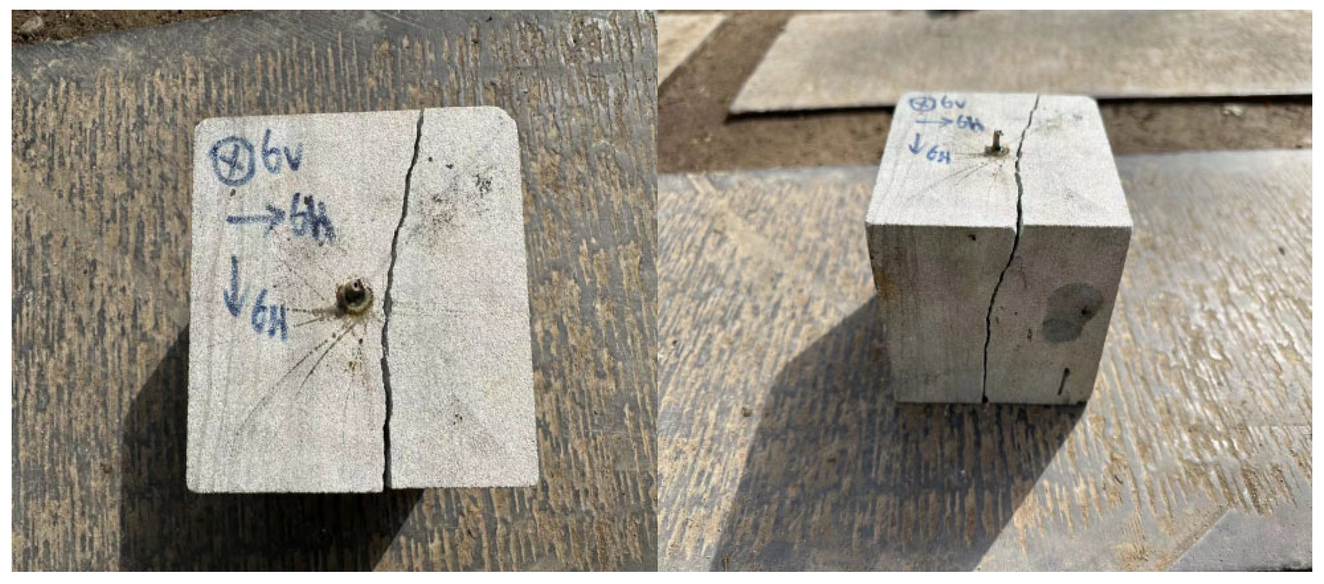
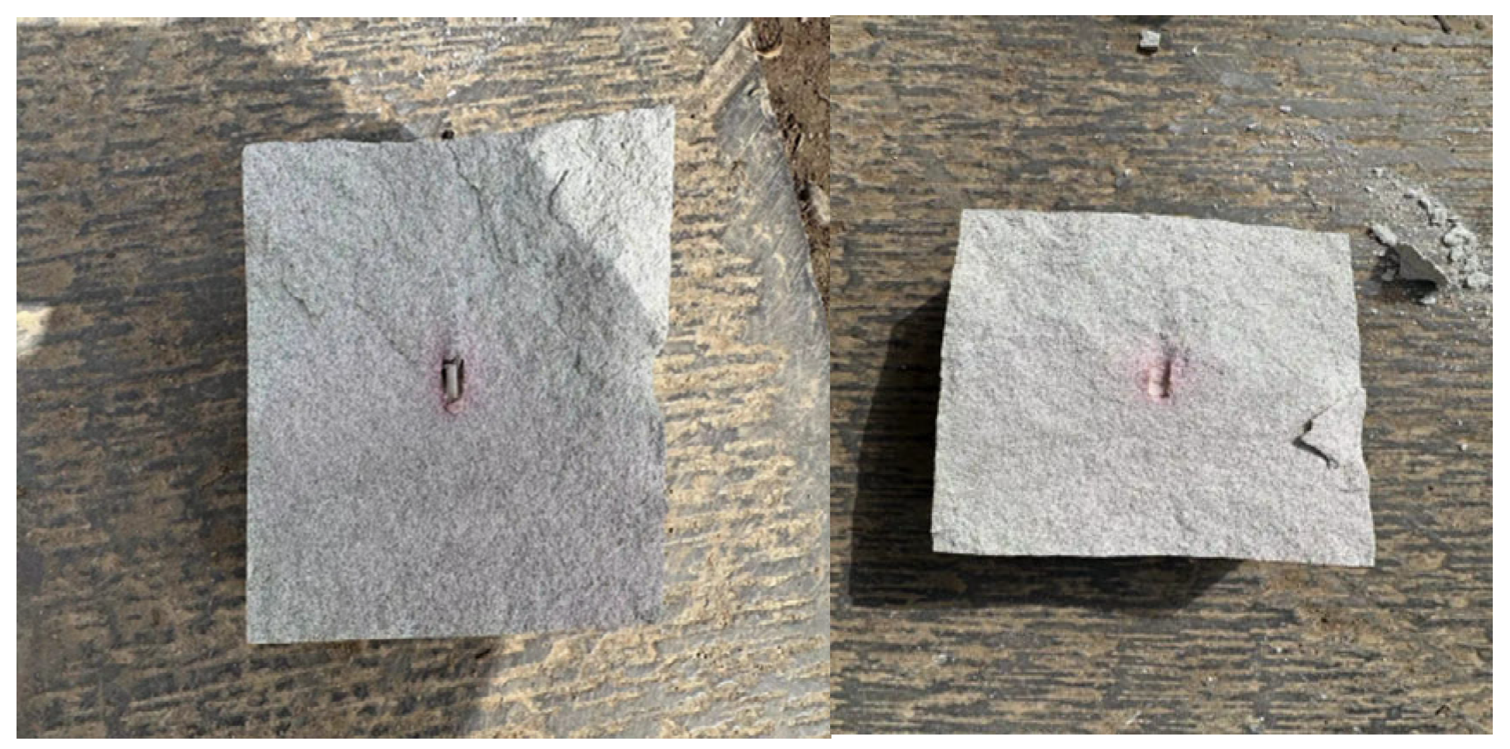
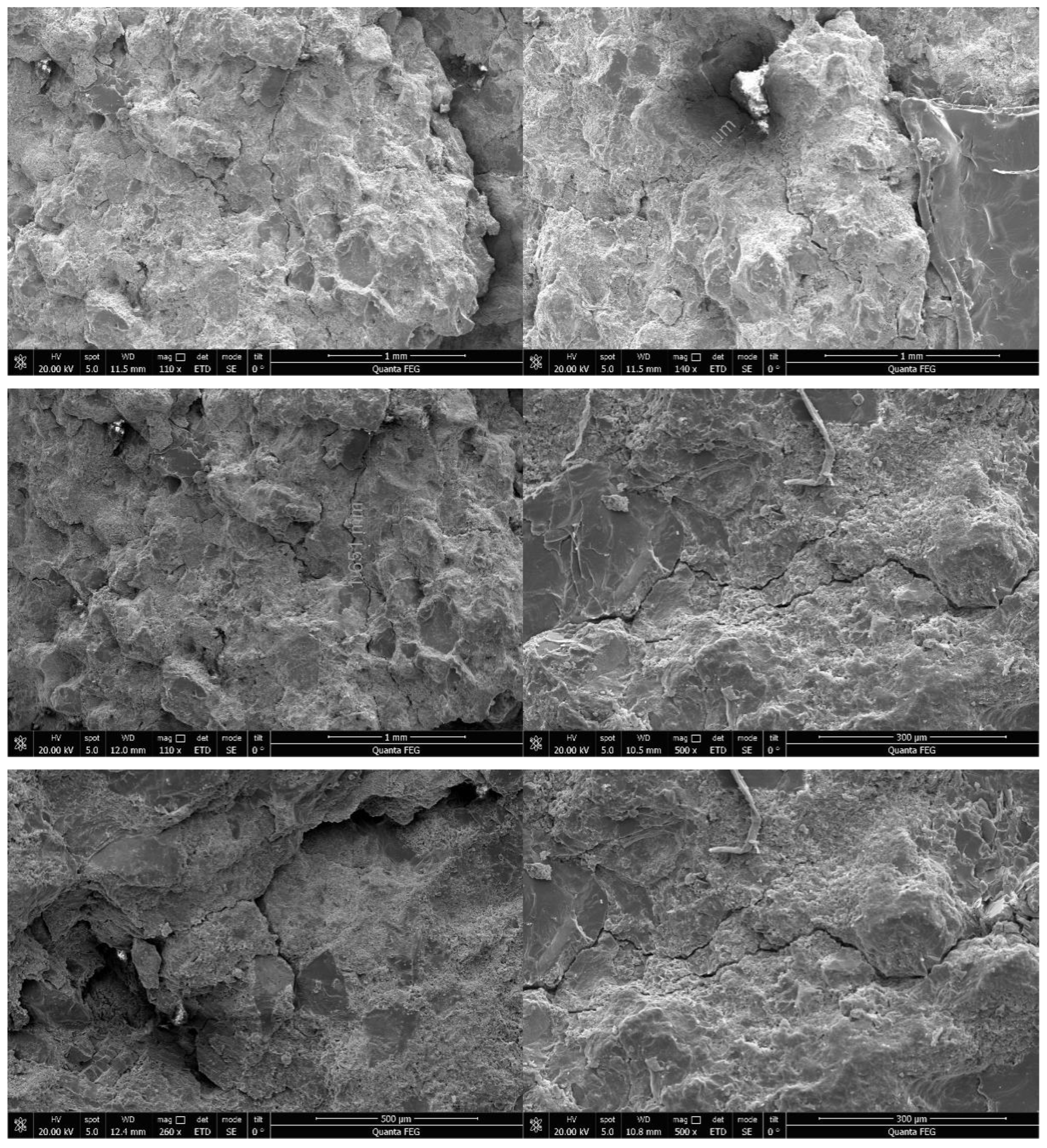
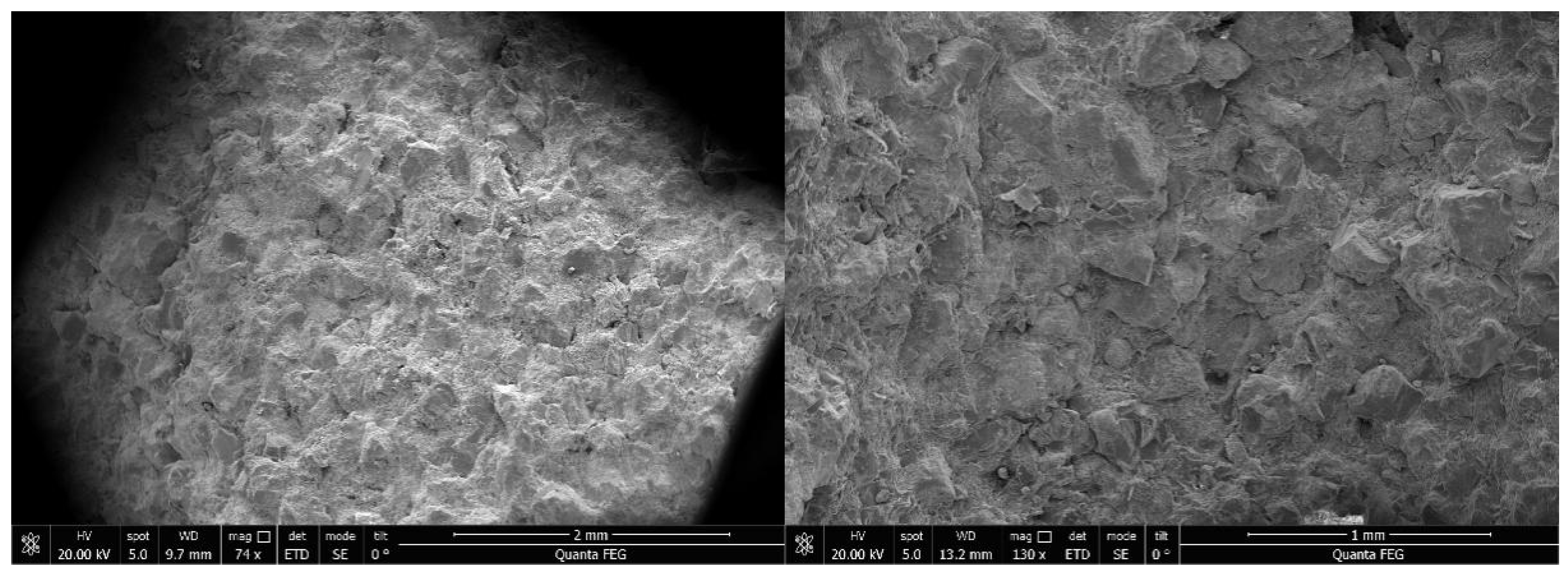
The true triaxial rock mechanics physical simulation experiment of water injection and dilatation showed that there were red areas (dilatation spread areas) on the surface of the sample after water injection, and no obvious cracks appeared in the sample. Electron microscope scans of the red zone of the rock cross-section and different water injection blocks after the test found that there were evident cracks in the block from near the wellbore but no cracks in the block far from the wellbore. At the same time, the 3D X-ray microscope and scanning results confirmed each other, where the more obvious the red area, the greater the fracture probability, while the principal wellbore (no red area) had almost no obvious fracture zone.

This study provides strong support for the subsequent development of target reservoir blocks using water injection capacity dilation technology and provides guidance for on-site construction.

References

1. Shentu, J.; Lin, B.; Lu, J. Research on risk assessment and prevention methods of shallow water flow hazards in deep-water and shallow areas. Pet. Sci. Bull. 2021, 3, 451–464. [Google Scholar]
2. Liu, W.H.; Yi, F.; Zhao, X.; He, R.; Li, C.; Liu, Y. Plugging removal and injection enhancement technology for the water injection wells in Bohai oilfield. Oil Drill. Prod. Technol. 2004, 26, 53–56. [Google Scholar]
3. Huang, R.Z. Initiation and dilation of hydraulic fracturing. Pet. Explor. Dev. 1982, 8, 65–77. [Google Scholar]
4. Samieh, A.M.; Wong, R.C.K. Modelling the Responses of Athabasca Oil Sand in Triaxial Compression Tests at Low Pressure. Can. Geotech. J. 1998, 35, 395–406. [Google Scholar] [CrossRef]
5. Wong, R.C.K. Strain-Induced Anisotropy in Fabric and Hydraulic Parameters of Oil Sand in Triaxial Compression. Can. Geotech. J. 2003, 40, 489–500. [Google Scholar] [CrossRef]
6. Yuan, Y.; Yang, B.; Xu, B. Fracturing in the oil sand reservoirs. In Proceedings of the Canadian Unconventional Resources Conference, Calgary, AB, Canada, 15–17 November 2011. SPE-149308-MS. [Google Scholar] [CrossRef]
7. Yuan, Y.; Xu, B.; Yang, B. Geomechanics for the thermal stimulation of heavy oil reservoirs. In Proceedings of the SPE Heavy Oil Conference and Exhibition, Kuwait City, Kuwait, 12–14 December 2011. SPE 150293 2011. [Google Scholar]
8. Wong, R.C.K.; Barr, W.E.; Kry, P.R. Stress-Strain Response of Cold Lake Oil Sand. Can. Geotech. J. 1993, 30, 220–235. [Google Scholar] [CrossRef]
9. ASTM D7181-11; Method for Consolidated Drained Triaxial Compression Test for Soils. ASTM International: West Conshohocken, PA, USA, 2003. [CrossRef]
10. ASTM D7012-14e1; Standard Test Methods for Compressive Strength and Elastic Moduli of Intact Rock Core Specimens under Varying States of Stress and Temperatures. ASTM International: West Conshohocken, PA, USA, 2014.
11. Xu, B.; Yuan, Y.; Wong, R.C.K. Modeling of the hydraulic fractures in unconsolidated oilsands reservoirs. In Proceedings of the 44th US Rock Mechanics Symposium and 5th U.S.—Canada Rock Mechanics Symposium, Salt Lake City, UT, USA, 27–30 June 2010. [Google Scholar]
12. Xu, B.; Wong, R.C.K. Coupled finite-element simulation of injection well testing in unconsolidated oil sands reservoir. Int. J. Numer. Anal. Methods Geomech. 2013, 37, 3131–3149. [Google Scholar] [CrossRef]
13. Xu, B.; Dou, S.; Zhang, J.; Chen, S. Consideration of geomechanics for in-situ bitu-men recovery in Xinjiang, China. In Proceedings of the SPE Heavy Oil Conferenc—Canada, Calgary, AB, Canada, 11–13 June 2013. SPE 165414. [Google Scholar]
14. Ulusay, R. The ISRM Suggested Methods for Rock Characterization, Testing and Monitoring: 2007–2014; Springer: Cham, Switzerland, 2015. [Google Scholar]
15. Duncan, J.M.; Chang, C.Y. Nonlinear Analysis of Stress and Strain in Soils. J. Soil Mech. ASCE 1970, 96, 1629–1653. [Google Scholar] [CrossRef]
16. Rowe, P.W. The Stress-Dilatancy Relation for Static Equilibrium of an Assembly of Particles in Contact. Proc. R. Soc. A Math. Phys. Eng. Sci. 1962, 269, 1339. [Google Scholar]
17. Bolton, M.D. The strength and dilatancy of sands. Geotechnique 1986, 36, 65–78. [Google Scholar] [CrossRef]
18. Lin, B.T.; Chen, S.; Pan, J.J.; Jin, Y.; Zhang, L.; Huiwen, P. Experimental study on dilation mechanism of micro-fracturing in continental ultra-heavy oil sand reservoir, Fengcheng Oilfield. Oil Drill. Prod. Technol. 2016, 38, 359–364. [Google Scholar]
19. Lin, B.T.; Jin, Y.; Chen, S.; You, H.; Huang, Y. Prediction on the reservoir dilatation results by squeeze preprocessing in SAGD wells. Oil Drill. Prod. Technol. 2018, 40, 341–347. [Google Scholar]
20. Lin, B.T.; Jin, Y. Evaluation of the Influencing Factors of Dilatancy Effects by Squeezing Liquids in SAGD Wells in the Fengcheng Oilfield of Xinjiang Oilfield. Pet. Drill. Tech. 2018, 46, 71–76. [Google Scholar]
21. Lin, B.T. Microfracturing mechanisms and techniques in unconsolidated sandstone formations. Pet. Sci. Bull. 2021, 6, 209–227. [Google Scholar]
22. Wang, Q.Q.; Lin, B.T.; Jin, Y.; Chen, S.; Pan, J. Effects of SAGD well squeeze dilatation on the circulating preheating and production. Oil Drill. Prod. Technol. 2019, 41, 387–392. [Google Scholar]
23. Ding, W.; Fan, T.; Huang, X.; Liu, C. Paleo-structural stress field simulation for middle-lower Ordovician in Tazhong area and favorable area prediction of fractured reservoirs. J. China Univ. Pet. (Ed. Nat. Sci.) 2010, 34, 1–6. [Google Scholar]
24. Zhao, A.; Xie, B.; He, X.; Wu, Y. Well logging evaluation of the Lower Permian dolomite reservoir in central Sichuan Basin. Nat. Gas Explor. Dev. 2017, 40, 1–6. [Google Scholar]
25. Zhu, X. Distribution laws of geomechanical parameters in Shihezi 1 Member, Fuxian block. Nat. Gas Explor. Dev. 2018, 41, 85–89. [Google Scholar]
26. Zhang, A.; Zhang, Y.; Liu, X.; Zhang, P. Test study on water affected to physical mechanics performances of muddy siltstone. Coal Sci. Technol. 2015, 43, 67–71. [Google Scholar]
27. Thomas, J. The birth of X-ray crystallography. Nature 2012, 491, 186–187. [Google Scholar] [CrossRef]
28. Pan, F.; Wang, Y.H.; Chen, C. X-ray Diffraction Technology; Chemical Industry Press: Beijing, China, 2016. [Google Scholar]
29. ASTM UOP905-20; Platinum Agglomeration by X-ray Diffraction. ASTM: West Conshohocken, PA, USA, 2020.
30. Shu, X.; Wu, Y.; Cheng, J.; Xia, Y.; Zheng, Y. Masterizer 2000 laser particle size analyzer and its applications. J. Hefei Univ. Technol. 2007, 30, 164–166. [Google Scholar]
31. Wang, W.; Li, Y.; Wang, Z.; Nie, Z.; Chen, B.; Yan, Z.; Yan, L.; Shao, C.; Lu, S. Evaluation of rock brittleness and analysis of related factors for tight sandstone reservoirs. China Pet. Explor. 2016, 21, 50–57. [Google Scholar]
32. Diao, H. Rock mechanical properties and brittleness evaluation of shale reservoir. Acta Petrol. Sin. 2013, 29, 3300–3306. [Google Scholar]
33. Jia, C. Foreland thrust-fold belt features and gas accumulation in Midwest China. Pet. Explor. Dev. 2005, 32, 9–15. [Google Scholar]
34. He, Y.; Wang, W. Sedimentary Rocks and Sedimentary Phases; Petroleum Industry Press: Beijing, China, 2006; (In Chinese with English Abstract). [Google Scholar]
35. Chen, Q.; Tang, W.; Xue, C.; Yang, Y.; Gao, W.; Yang, J.; Jia, J. The ϕ Value Expresses Granularity and the Unit Problem of the Sorting Coefficient. Acta Sedimentol. Sin. 2022, 1–16. [Google Scholar] [CrossRef]
36. Trask, P.D. Mechanical analyses of sediments by centrifuge. Econ. Geol. 1930, 25, 581–599. [Google Scholar] [CrossRef]
37. Inman, D.L. Measures for describing the size distribution of sediments. J. Sediment. Res. 1952, 22, 125–145. [Google Scholar]
38. Folk, R.L.; Ward, W.C. Brazos river bar: A study in the significance of grain size parameters. J. Sediment. Res. 1957, 27, 3–26. [Google Scholar] [CrossRef]
39. GB/T 12763.8; Specifications for Oceanographic Survey—Part 8: Marine Geology and Geophysics Survey. National Standards of People’s Republic of China: Beijing, China, 2008.
Figure 1. Sample grinding (left) 200 mesh powder sample (right).
Processes 12 02015 g001
Figure 2. Filling samples.
Processes 12 02015 g002
Figure 3. D8 ADVANCE X-ray powder diffractometer.
Processes 12 02015 g003
Figure 4. Quantitative analysis results for (1) sample 1, (2) sample 2, (3) sample 3, (4) sample 4, (5) sample 5, and (6) sample 6.
Processes 12 02015 g004
Figure 5. Hydrochloric acid cleaning (left), hydrogen peroxide neutralization and cleaning (middle), and ultrasonic cleaning (right) were used.
Processes 12 02015 g005
Figure 6. Mastersize2000 laser particle size analyzer.
Processes 12 02015 g006
Figure 7. Normal triaxial stress state diagram.
Processes 12 02015 g007
Figure 8. True triaxial stress state diagram.
Processes 12 02015 g008
Figure 9. Preinjection samples.
Processes 12 02015 g009
Figure 10. Sample during water injection.
Processes 12 02015 g010
Figure 11. The true three-axis multifunction comprehensive experimental platform and HADSZ-II electrical control system.
Processes 12 02015 g011
Figure 12. Schematic of the biaxial synchronous loading.
Processes 12 02015 g012
Figure 13. Histograms of the mineral content of (1) sample #1, (2) sample #2, (3) sample #3, (4) sample #4, (5) sample #5, and (6) sample #6.
Processes 12 02015 g013
Figure 14. Sample brittleness.
Processes 12 02015 g014
Figure 15. Percentage by volume (blue) and cumulative volume percentage (red) of (1) sample #1, (2) sample #2, (3) sample #3, and (4) sample #4.
Processes 12 02015 g015
Figure 16. Diagram of the direction and magnitude of the three-phase stress applied to sample 1.
Processes 12 02015 g016
Figure 17. (a) The real-time liquid flow rate of sample #2, (b) real-time pump pressure curve of sample #2, (c) cumulative liquid flow rate of sample #2, and (d) image of sample #3.
Processes 12 02015 g017
Figure 18. (a) The real-time liquid flow rate of sample #3, (b) real-time pump pressure curve of sample #3, (c) cumulative liquid flow rate of sample #3, and (d) image of sample #3.
Processes 12 02015 g018
Figure 19. Post-injection sample.
Processes 12 02015 g019
Figure 20. Cracked-open sample (whole).
Processes 12 02015 g020
Figure 21. Cracked-open sample (apart).
Processes 12 02015 g021
Figure 22. Sample preparation.
Processes 12 02015 g022
Figure 23. Samples taken from near the wellbore.
Processes 12 02015 g023
Figure 24. Samples collected far from the wellbore.
Processes 12 02015 g024
Figure 25. The Xradia 520 Versa X-ray microscope.
Processes 12 02015 g025
Figure 26. Samples collected far from the wellbore.
Processes 12 02015 g026