Refractured Well Hydraulic Fractures Optimization in Tight Sandstone Gas Reservoirs: Application in Linxing Gas Field

Abstract

Poorly producing wells in sandstone gas reservoirs are often refractured to enhance production. Considering the mutual interference of initial/refractured fractures, conductivity dynamic evolution, non-uniform inflow, and variable mass flow in the fracture comprehensively, a semi-analytical reservoir-fracture coupled production model fusing spatial and time separation methods is introduced to model refractured well performance. The proposed model is verified by CMG. The field applications indicate that the refracture job should be carried out when production is lower than the desired value. Restoring the C_f-ini and constructing the C_f-ref can increase productivity, which increases over 8 D•cm. The production growth rate just obtained a slight improvement. The production increased significantly with L_f-ini increasing from 120~270 m and L_f-ref increasing from 100~150 m. Hence, it is essential to extend the L_f-ini under engineering conditions. The k_s/k_m = 10 can obviously increase production, but further enlarging k_s does not contribute to well performance. Conversely, further producing larger b_s is vital to enhancing production. Subsequently, the optimal parameter combinations (d_s > L_f-ini > L_f-ref > C_f-ini > k_s > C_f-ref) for well(X1) are carried out by orthogonal experiments. This work proposes a novel method to simulate refractured vertical well performance in tight gas reservoirs for refracture optimization.

1. Introduction

Tight sand gas reservoirs have been discovered in many basins worldwide, which are defined as reservoirs without economic flow rates or economically recoverable volumes of natural gas unless wells are fractured [1,2]. The reservoir permeability magnitude is central to the fracture morphology, and flow from the reservoir to the wellbore can be achieved by stimulating long fractures with high conductivity. To maintain the fracture conductivity, the injected fracturing fluid must be recovered, and proppants must remain in the fracture to prevent fracture closure during hydrocarbon production upon the termination of the stimulation job [3,4].

On most occasions, hydraulically fractured wells in gas reservoirs suffer a steep production decline during production [5], which does not meet the desired expectation [6,7]. There are several reasons for this phenomenon. As the fracturing fluid filtrates into the matrix, an increasing polymer concentration is formed on the proppant side, which alters the effective support length along the fracture due to different proppant and fracturing fluid concentrations. Under ideal conditions, the viscosity of fracturing fluids should decrease when the stimulation job is completed so that the fracturing fluids can flow back quickly to reduce the residual concentration [8]. Moreover, with increasing bearing time and closure pressure in tight gas development, proppant crushing and embedment reduce the conductivity [9]. Fortunately, multiple fracture stimulations can be carried out in tight gas wells. Numerous robust field cases are demonstrating that many developed gas wells can still yield considerable gas production that can be exploited by refracturing treatment. Refracturing can enhance the original fracture performance or create new fractures in the formation and is considered to add life and economically improve the well productivity when the initial stimulation effect is inadequate [10,11]. There are many reasons for this finding, such as a limited stimulation scale, poorly performing fracturing fluids, a low proppant concentration and poor distribution, unfavorable proppant selection, and an unreasonable perforation orientation and density [12,13]. Construction of the initial or new fractures increases the extension of the fracture geometry, thereby contacting unexploited reservoir regions and increasing the fracture conductivity, and the key attributes of refracturing success include the number of connected, undeveloped reservoirs [14]. Refracturing is a widely accepted technique to repair or replace an inadequate initial fracturing treatment. The hydraulic fracture direction always coincides with the direction of the maximum principal stress. There are two kinds of refractures. One type is the refracture initiating from the wellbore and orthogonally propagating toward the initial fracture, while the other refracture type propagates parallel to the initial fracture from the tip of the latter fracture [15,16]. The second well refracturing method employs diverting agents, the refractured fractures along the initial fracture remain open, and fracturing fluids enter simultaneously. Diverting agents are applied to block the initial fractures and facilitate the new refracture branches [17,18]. Regarding the ultralow permeability of tight gas reservoirs, the second fracture type is highly desirable because connectivity with the rock matrix suggests contact area and productivity enhancement [19,20].

Although great efforts have been made to study refractures and ultimately improve production mechanisms [5,21], candidate well identification [22,23], and refracturing treatment design [24,25,26], very few investigators have focused on the production performance evaluation of refractured wells [27]. Numerical methods are powerful tools to study the production performance of fractured wells. However, due to the complexity of the flow regime, which requires notable computational and time resources, the numerical approach is difficult to widely implement in practical engineering [8,28,29,30]. To overcome the drawbacks of the numerical simulation method, semianalytical methods have been developed to couple the various flow regimes of reservoirs and hydraulic fractures, which can describe the transient flow characteristics of different fractures [28]. In these models, hydraulic fractures are effectively discretized into several segments, which coexist in both the matrix and fracture systems. The Green function and Newman product method have been applied to model fluid flow in the matrix system, while one-dimensional flow equations capture the fluid flow in the fracture; moreover, matrix and fracture flow equations have been coupled based on flux and pressure continuity [28,31,32,33,34,35]. Teng [15] discretized original fractures and refractures into segments and developed semianalytical models to appraise the performance of orthogonally refractured vertical wells.

However, the following issues have not been suitably addressed in the aforementioned models: First, refracturing-induced complex fracture networks can be produced and developed via refracturing treatment aided by temporary diverting agents, which increases both the contact area and connectivity between the fractures and reservoirs. This also suggests notable productivity enhancement. Hence, the assumption of only single fractures in the above models is inappropriate, which inadequately describes the fracturing volume (complex fracture networks) of refractured wells [27]. Second, these models typically ignore the conductivity decay evolution of existing and refractured fractures. Conductivity test experiments and actual field production cases have revealed that the proppant-induced fracture conductivity weakens over time, leading to well production attenuation [9,36].

In this paper, we incorporate the Newman integral method with Green’s function to simulate the flow characteristics of refractured wells. Based on mass balance and pressure continuity considerations, the initial fracture and refracture are discretized into several segments, and the Duhamel principle is applied to address the flow superimposition phenomenon during refracturing. Additionally, the refracturing-induced fracture networks are treated as negative skin factors, and an attenuation equation of the conductivity is determined through long-term conductivity tests on slate samples. Finally, the presented model was successfully applied to well(X1) for production simulation and design optimization in the Sichuan basin of China.

2. Methodology

The following basic assumptions are made to ensure the rationality of the mathematical model:

(1)

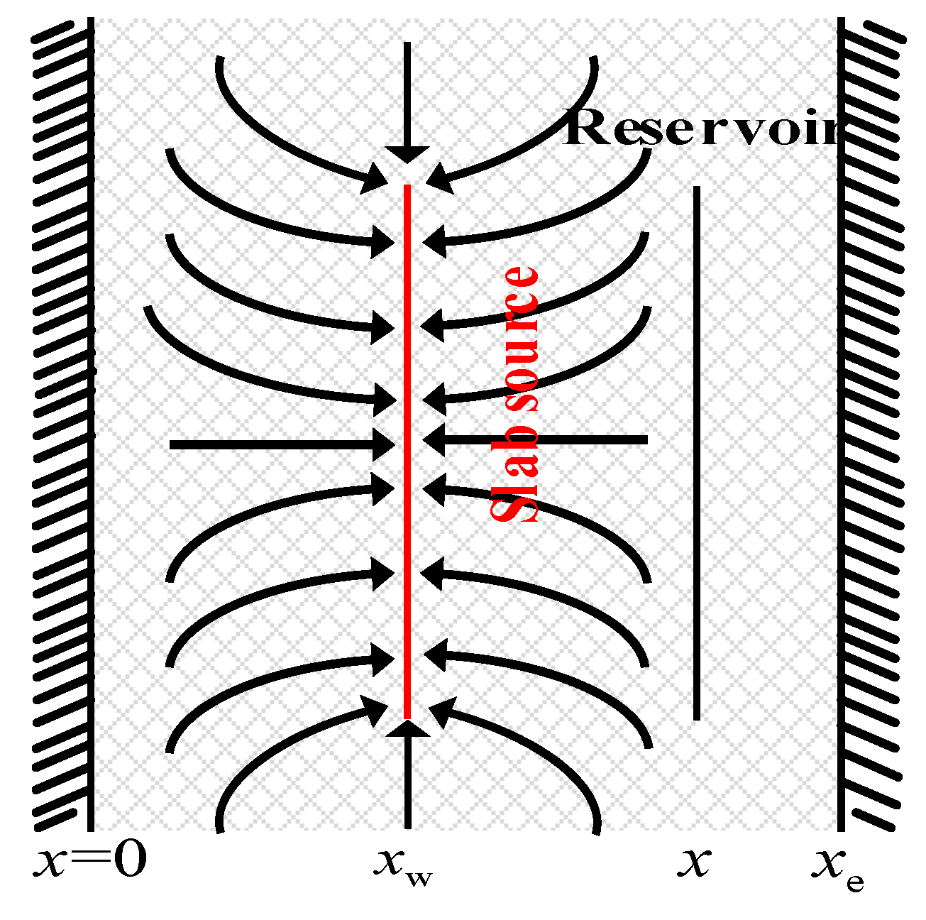
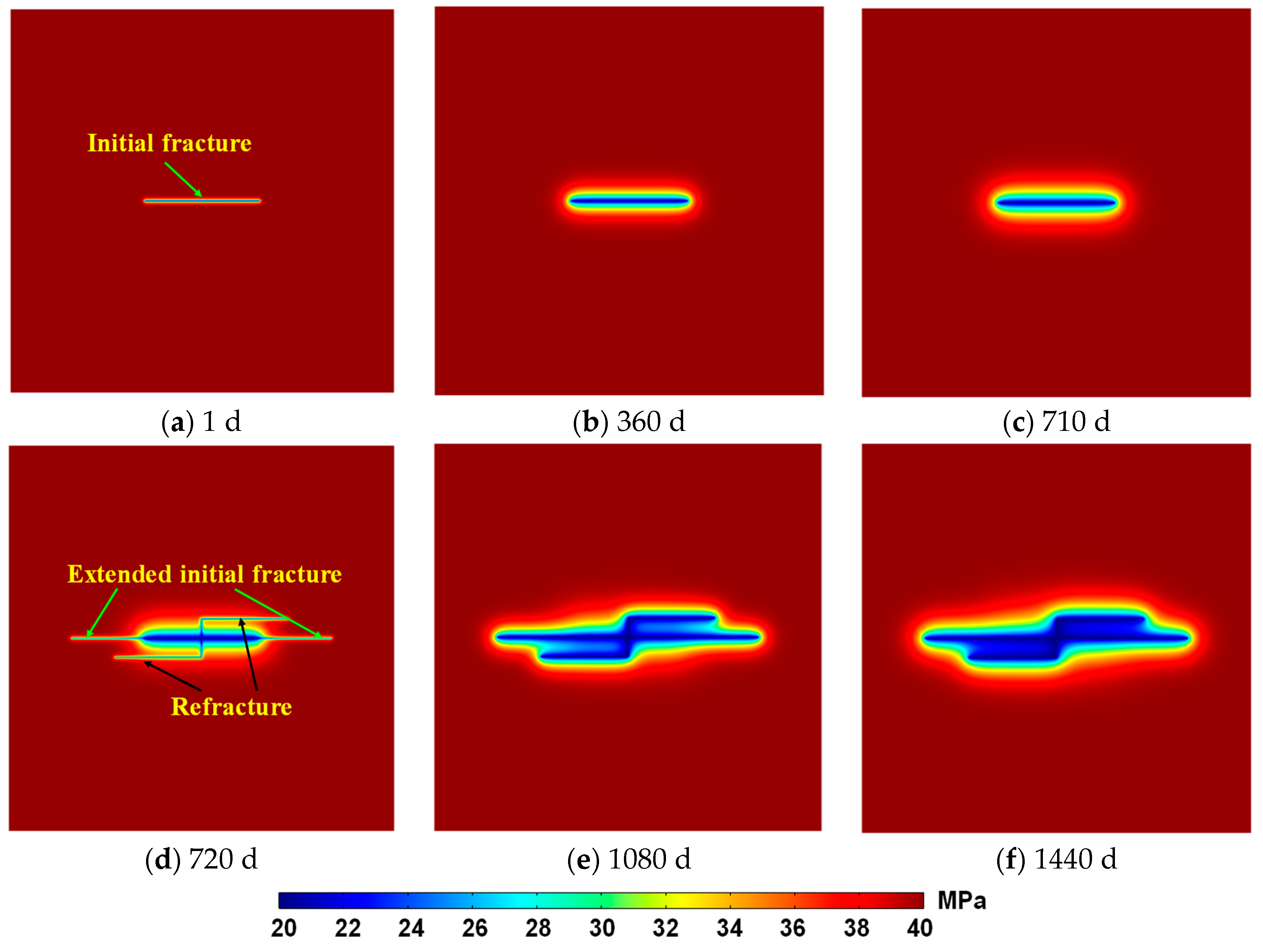
The reservoir boundary exhibits a constant width and length, the hydraulic fracture fully penetrates the reservoir, and the fracture branch after refracturing is shown in Figure 1;

(2)

The height, porosity, and permeability do not change in homogeneous and isotropic reservoirs;

(3)

Compressible single-phase gas flow occurs in reservoirs with a constant compressibility coefficient and viscosity;

(4)

Complex secondary fractures with enhanced permeability are created by refracturing;

(5)

The main fracture’s dynamic conductivity decreases over time.

The hydraulic fracture is discretized into a series of nodes, and there are ns nodes in the main fracture and m nodes in the refracture branch. Subscript k represents the fracture node index, which ranges from 1 to ns + m.

3. Mathematical Model

A refractured vertical gas well in a reservoir with a closed top and bottom is characterized by three integrated processes: reservoir seepage flow, refracturing-induced fracture network flow, and main fracture flow. Therefore, the corresponding semi-analytical solutions are coupled based on mass balance and pressure continuity.

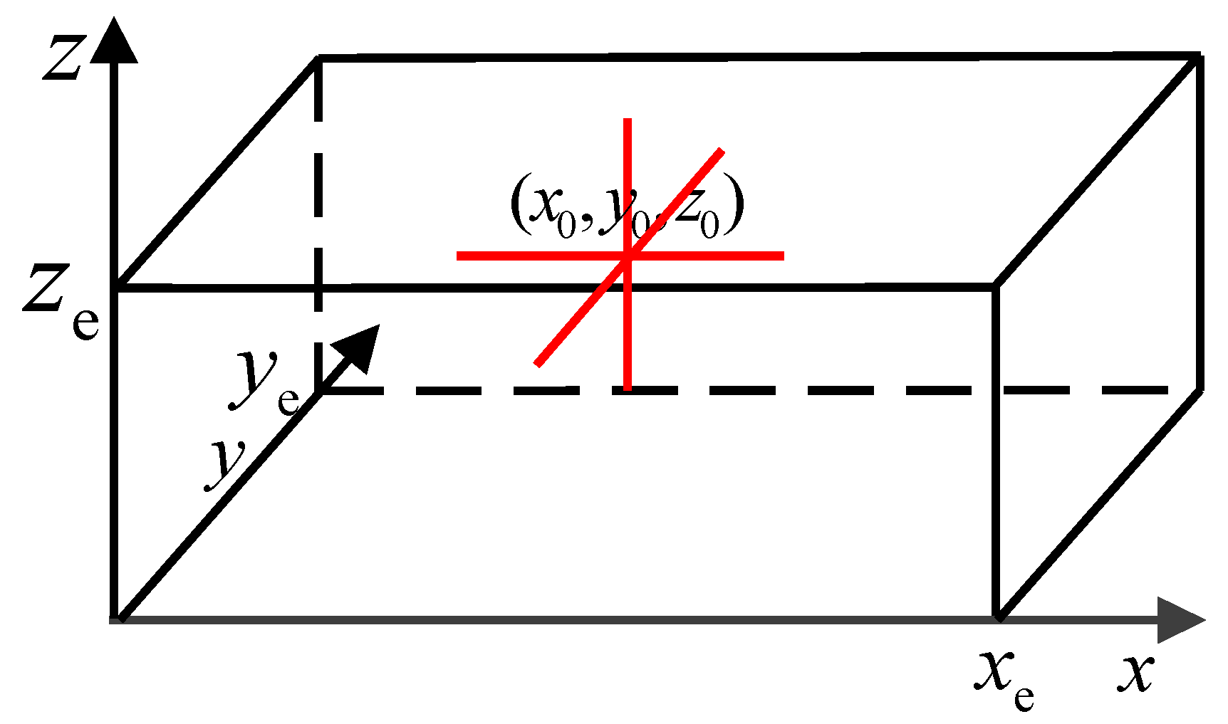
3.1. Reservoir Seepage Model

The unsteady-state gas flow in homogeneous and isotropic reservoirs can be represented by the pseudo-pressure function-based diffusion equation as follows [37]:

$$\left\{\begin{array}{l}{\eta }_x{\displaystyle \frac{{\partial }^2\tilde{p}}{\partial x^2}}+{\eta }_y{\displaystyle \frac{{\partial }^2\tilde{p}}{\partial y^2}}+{\eta }_z{\displaystyle \frac{{\partial }^2\tilde{p}}{\partial z^2}}={\displaystyle \frac{\partial \tilde{p}}{\partial t}}\\ \tilde{p}\left(x_{\mathrm{e}},y_{\mathrm{e}},z_{\mathrm{e}},t\right)={\tilde{p}}_{\mathrm{in}}\\ \tilde{p}\left(x,y,z,t=0\right)={\tilde{p}}_{\mathrm{in}}\\ \tilde{p}\left(x_{\mathrm{w}},y_{\mathrm{w}},z_{\mathrm{w}},t\right)={\tilde{p}}_{\mathrm{wf}}\end{array}\right.$$

(1)

Pressure coefficient in three dimensions, respectively [38].

$${\eta }_x={\eta }_y={\eta }_z={\displaystyle \frac{k_{\mathrm{m}}}{\varphi {\mu }_g{c}_{\mathrm{t}}}}$$

(2)

Slab source solutions in the x, y, and z dimensions can be obtained by Green’s function and the Newman integral method, and the three one-dimensional slab source solutions over time can be integrated to create a unique three-dimensional point source solution function. The pseudo-pressure drop under constant production q in homogenous and isotropic reservoirs at positions (x, y, z) is expressed as follows [39,40]:

$${\tilde{p}}_{\mathrm{in}}-\tilde{p}\left(x, y, z, t\right)={\displaystyle \frac{q{B}_{\mathrm{g}}}{\phi c_{\mathrm{t}}\Delta xhw}}{\displaystyle {\int }_0^t{\displaystyle {\int }_{z_1}^{z_2}{\displaystyle {\int }_{y_1}^{y_2}{\displaystyle {\int }_{x_1}^{x_2}S(x,t)\cdot S(y,t)\cdot S(z,t)}}}}\mathrm{d}t\mathrm{d}x\mathrm{dydz}$$

(3)

$$B_{\mathrm{g}}={\displaystyle \frac{p_{\mathrm{sc}}TZ}{p_{\mathrm{air}}{T}_{\mathrm{sc}}{Z}_{\mathrm{sc}}}}$$

(4)

The pseudo-pressure function in gas reservoirs can be expressed as follows [41]:

$$\tilde{p}=2{\displaystyle {\int }_0^p\frac{p}{\mu Z}}\mathrm{d}p={\displaystyle \frac{2p^2}{\mu Z}}$$

(5)

Substituting Equations (4) and (5) into Equation (3), the following can be obtained:

$$p_{\mathrm{in}}^2-p^2\left(x, y, z, t\right)={\displaystyle \frac{q\mu p_{\mathrm{sc}}T}{\phi c_{\mathrm{t}}\Delta xhw{p}_{\mathrm{air}}{T}_{\mathrm{sc}}{Z}_{\mathrm{sc}}}}{\displaystyle {\int }_0^t{\displaystyle {\int }_{z_1}^{z_2}{\displaystyle {\int }_{y_1}^{y_2}{\displaystyle {\int }_{x_1}^{x_2}S(x,t)\cdot S(y,t)\cdot S(z,t)}}}}\mathrm{d}t\mathrm{d}x\mathrm{dydz}$$

(6)

where:

$$S(x,t)={\displaystyle \frac{1}{x_{\mathrm{e}}}}\left(1+2{\displaystyle \sum _{n=1}^{\infty }\exp (-\frac{n^2{\mathsf{\pi }}^2{\eta }_{x}t}{{x_{\mathrm{e}}}^2})\cdot \cos \frac{n\mathsf{\pi }x}{x_{\mathrm{e}}}\cdot \cos \frac{n\mathsf{\pi }{x}_{\mathrm{w}}}{x_{\mathrm{e}}}}\right)$$

(7)

$$S(y,t)={\displaystyle \frac{1}{y_{\mathrm{e}}}}\left(1+2{\displaystyle \sum _{n=1}^{\infty }\exp (-\frac{n^2{\mathsf{\pi }}^2{\eta }_{y}t}{{y_{\mathrm{e}}}^2})\cdot \cos \frac{n\mathsf{\pi }y}{y_{\mathrm{e}}}\cdot \cos \frac{n\mathsf{\pi }{y}_{\mathrm{w}}}{y_{\mathrm{e}}}}\right)$$

(8)

$$S(z,t)={\displaystyle \frac{1}{z_{\mathrm{e}}}}\left(1+2{\displaystyle \sum _{n=1}^{\infty }\exp (-\frac{n^2{\mathsf{\pi }}^2{\eta }_{z}t}{{z_{\mathrm{e}}}^2})\cdot \cos \frac{n\mathsf{\pi }z}{z_{\mathrm{e}}}\cdot \cos \frac{n\mathsf{\pi }{z}_{\mathrm{w}}}{z_{\mathrm{e}}}}\right)$$

(9)

Newman’s integral method is applied to obtain the custom point source solution [33], and by substituting Equations (7)–(9) into and then integrating Equation (6), the solution can be rewritten as:

$$p_{\mathrm{in}}^2-p^2\left(x, y, z, t\right)=q_{\mathrm{f}k}\cdot F_k\left(x, y, z, t\right)$$

(10)

The coefficient $F_k\left(x, y, z, t\right)$ is presented in Appendix A.

Based on Duhamel’s principle, one can transform the constant-production condition into a variable output. At the time $\Delta t$, we derive the following [42]:

$$\begin{array}{l}\Delta p_k\left(\Delta t\right)=p_{\mathrm{in}}^2-p_k^2\left(\Delta t\right)\\ =q_{\mathrm{f}1}\left(\Delta t\right)F_1\left(\Delta t\right)+q_{\mathrm{f}2}{F}_2\left(\Delta t\right)+q_{\mathrm{f}3}{F}_3\left(\Delta t\right)+\cdot \cdot \cdot +q_{\mathrm{f}k}{F}_k\left(\Delta t\right)+\cdot \cdot \cdot +q_{\mathrm{f}ns+m}{F}_{ns+m}\left(\Delta t\right)\hfill \end{array}$$

(11)

At $\mathrm{time}=n\Delta t$, which is the n-th time step, one can obtain the following [43]:

$$\begin{array}{l}\Delta p_k\left(n\Delta t\right)=p_{\mathrm{in}}^2-p_k^2\left(n\Delta t\right)\\ =\left\{q_{\mathrm{f}1}\left(\Delta t\right)F_{11,k+1j}\left(n\Delta t\right)+\left[q_{\mathrm{f}2}\left(2\Delta t\right)-q_{\mathrm{f}1}\left(\Delta t\right)\right]F_1\left(\left(n-1\right)\Delta t\right)\right.\\ \begin{array}{cccc}& & & \end{array}+\left[q_{\mathrm{f}1}\left(3\Delta t\right)-q_{\mathrm{f}1}\left(2\Delta t\right)\right]F_1\left(\left(n-2\right)\Delta t\right)+.....\\ \left.\begin{array}{cccc}& & & \end{array}+\left[q_{\mathrm{f}1}\left(n\Delta t\right)-q_{\mathrm{f}1}\left(\left(n-1\right)\Delta t\right)\right]F_1\left(\Delta t\right)\right\}\\ \begin{array}{cccc}& & & \end{array}+\left\{q_{\mathrm{f}ns+m}\left(\Delta t\right)F_{ns+m}\left(n\Delta t\right)+\left[q_{ns+m}\left(2\Delta t\right)-q_{ns+m}\left(\Delta t\right)\right]F_{ns+m}\left(\left(n-1\right)\Delta t\right)\right.\\ \begin{array}{cccc}& & & \end{array}+\left[q_{\mathrm{f}ns+m}\left(3\Delta t\right)-q_{\mathrm{f}ns+m}\left(2\Delta t\right)\right]F_{ns+m}\left(\left(n-2\right)\Delta t\right)+.....\\ \left.\begin{array}{cccc}& & & \end{array}+\left[q_{\mathrm{f}ns+m}\left(n\Delta t\right)-q_{\mathrm{f}ns+m}\left(\left(n-1\right)\Delta t\right)\right]F_{ns+m}\left(\Delta t\right)\right\}\\ ={\displaystyle \sum _{k=1}^{ns+m}{q}_{\mathrm{f}k}\left(\Delta t\right)F_k(n\Delta t)+\left.{\displaystyle \sum _{g=2}^n\left[q_{\mathrm{f}k}\left(g\Delta t\right)-q_{\mathrm{f}k}\left((g-1)\Delta t\right)\right]F_k\left[(n-g+1)\Delta t\right]}\right\}}\end{array}$$

(12)

3.2. Induced Fracture Networks

The fracture networks after fracturing exhibit enhanced permeability. Cinco [44] delimited the fracture skin factor through penetration and permeability damage aspects. Van [45] defined the additional pressure drop caused by the resistance as the skin effect. Subsequently, the negative skin factor is introduced to treat the additional pressure drop in reservoirs attributed to fracturing-induced secondary fractures. At the k-th node, the fracture skin factor is as follows [32,46].

$$s_{\mathrm{ff}k}={\displaystyle \frac{\mathsf{\pi }{b}_{\mathrm{s}}}{2\Delta x_{\mathrm{f}k}}}({\displaystyle \frac{k_{\mathrm{m}}}{k_{\mathrm{s}}}}-1)$$

(13)

Gas flow in the matrix satisfies the following linear differential equation:

$$q_{\mathrm{f}k}={\displaystyle \frac{k_{\mathrm{m}}\Delta x_{\mathrm{f}k}h}{\mu }}{\displaystyle \frac{\mathrm{d}p}{\mathrm{d}l}}$$

(14)

Substituting $q_{\mathrm{f}k}={\displaystyle \frac{p_{\mathrm{sc}}}{T_{\mathrm{sc}}}}{\displaystyle \frac{ZT}{Z_{\mathrm{sc}}p}}{q}_{\mathrm{sc}}$ and Equation (14) into the integral along the secondary fracture width, one can obtain as follows:

$${\displaystyle \frac{q_{\mathrm{sc}}{p}_{\mathrm{sc}}Z\mathrm{T}}{T_{\mathrm{sc}}{Z}_{\mathrm{sc}}}}{\displaystyle {\int }_0^{b_{\mathrm{s}}}\mathrm{d}}l={\displaystyle \frac{k_{\mathrm{m}}\Delta x_{\mathrm{f}k}h}{\mu }}{\displaystyle {\int }_{p_{\mathrm{s}k}}^{p_{\mathrm{f}k}}p\mathrm{d}}p$$

(15)

The integral can obtain secondary fracture pressure drop with $k_{\mathrm{m}}$ as follows:

$$\Delta p_{\mathrm{sff}k}^2=p_{\mathrm{s}k}^2-p_{\mathrm{f}k}^2={\displaystyle \frac{2q_{\mathrm{sc}}\mu p_{\mathrm{sc}}Z\mathrm{T}{b}_{\mathrm{s}}}{h\Delta x_{\mathrm{f}k}{T}_{\mathrm{sc}}{Z}_{\mathrm{sc}}{k}_{\mathrm{m}}}}$$

(16)

The secondary fracture-induced additional pressure drop can be multiplied by the negative skin factor [45,47,48], one can obtain as follows:

$$\Delta p_{\mathrm{sff}k-\mathrm{add}}^2 ={\displaystyle \frac{2q_{\mathrm{sc}}\mu p_{\mathrm{sc}}Z\mathrm{T}{b}_{\mathrm{s}}}{h\Delta x_{\mathrm{f}k}{T}_{\mathrm{sc}}{Z}_{\mathrm{sc}}{k}_{\mathrm{m}}}}{s}_{\mathrm{ff}k}$$

(17)

3.3. Main Fracture Flow Model

In this section, we develop a semi-analytical solution for a refractured vertical well with finite conductive fractures. The flow process along the main fracture nodes is constructed by Darcy’s law, which considers dynamic conductivity attenuation over time.

The main fracture flow equation satisfies Darcy’s law, and the flow equation at each discrete node is as follows:

$${\displaystyle \frac{\mathrm{d}{p}_{\mathrm{fk}}}{\mathrm{d}{x}_{\mathrm{f}k}}}={\displaystyle \frac{\mu v_{\mathrm{f}k}}{k_{\mathrm{f}k}}}$$

(18)

$$v_{\mathrm{f}k}={\displaystyle \frac{q_{\mathrm{f}k}}{w_{\mathrm{f}k}{h}_{\mathrm{f}k}}}$$

(19)

The flow rates inside and outside an arbitrary fracture node satisfy mass balance conditions. Given ns initial fracture nodes and m refracture branch nodes, we can write the following equation:

$$q_{\mathrm{f}n}={\displaystyle \sum _{i=n}^{ns}{q}_{ri}}$$

(20)

In particular, all ns + m equations are satisfied.

p_rk+1 indicates the reservoir node pressure outside the fracture face. For the same node, p_fk+1, i.e., the fracture node pressure, is the sink point pressure for the whole fracture cross-section. Consequently, the pressure continuity between the reservoir and fracture is defined by setting the reservoir nodal pressure equal to the fracture nodal pressure. Given ns initial fracture nodes and m refracture branch nodes, one can write:

$$\left\{\begin{array}{l}{p}_{\mathrm{f}j}=p_{rj}\begin{array}{cc},& j\in (1,ns+m)\end{array}\\ p_{\mathrm{f}1}=p_{\mathrm{wf}}\end{array}\right.$$

(21)

Initial fracture and refracture branch flow equations can be obtained from mass balance and pressure continuity equations. Regarding the half-single fracture in our model, before the refracture job, the pressure drop equation from the j-th main fracture node to the bottom of the well can be expressed as follows [49]:

$$\begin{array}{l}\Delta p_{\mathrm{f}k}^2\left(t\le t_{\mathrm{refracture}}\right)=p_{\mathrm{f}k}^2-p_{\mathrm{wf}}^2\\ ={\displaystyle \frac{2{\mu }_g{p}_{\mathrm{sc}}\mathrm{ZT}}{k_{\mathrm{f}k}\left(t\right)w_{\mathrm{f}k}h{T}_{\mathrm{sc}}}}\Delta x_{\mathrm{f}1}{q}_{\mathrm{r}1}+{\displaystyle \frac{2{\mu }_g{p}_{\mathrm{sc}}\mathrm{ZT}}{k_{\mathrm{f}k}\left(t\right)w_{\mathrm{f}k}h{T}_{\mathrm{sc}}}}\left(\Delta x_{\mathrm{f}1}+\Delta x_{\mathrm{f}2}\right)q_{\mathrm{r}2}+\cdots +{\displaystyle \frac{2{\mu }_g{p}_{\mathrm{sc}}\mathrm{ZT}}{k_{\mathrm{f}k}\left(t\right)w_{\mathrm{f}k}h{T}_{\mathrm{sc}}}}\left(\Delta x_{\mathrm{f}1}+\Delta x_{\mathrm{f}2}+\cdots +\Delta x_{\mathrm{f}j}\right)q_{\mathrm{r}j}\\ +{\displaystyle \frac{2{\mu }_g{p}_{\mathrm{sc}}\mathrm{ZT}}{k_{\mathrm{f}k}\left(t\right)w_{\mathrm{f}k}h{T}_{\mathrm{sc}}}}\left(\Delta x_{\mathrm{f}1}+\Delta x_{\mathrm{f}2}+\cdots +\Delta x_{\mathrm{f}j}\right)q_{\mathrm{r}j+1}+\cdots +{\displaystyle \frac{2{\mu }_g{p}_{\mathrm{sc}}\mathrm{ZT}}{k_{\mathrm{f}k}\left(t\right)w_{\mathrm{f}k}h{T}_{\mathrm{sc}}}}\left(\Delta x_{\mathrm{f}1}+\Delta x_{\mathrm{f}2}+\cdots +\Delta x_{\mathrm{f}j}\right)q_{\mathrm{r}ns}\\ ={\displaystyle \frac{2{\mu }_g{p}_{\mathrm{sc}}\mathrm{ZT}}{k_{\mathrm{f}k}\left(t\right)w_{\mathrm{f}k}h{T}_{\mathrm{sc}}}}{\displaystyle \sum _{i=1}^{ns}\left( q_{\mathrm{r}i}{\displaystyle \sum _{j=1}^i\Delta x_{\mathrm{f}j}} \right)}\end{array}$$

(22)

The refractures are constructed by refracturing, the pressure drop equation from the j-th main fracture node and the i-th branch fracture node to the well bottom can be expressed as follows:

$$\begin{array}{l}\Delta p_{\mathrm{f}k}^2\left(t>t_{\mathrm{refracture}}\right)=p_{\mathrm{f}k}^2-p_{\mathrm{wf}}^2\\ ={\displaystyle \frac{2{\mu }_g{p}_{\mathrm{sc}}\mathrm{ZT}}{k_{\mathrm{f}k}\left(t\right)w_{\mathrm{f}k}h{T}_{\mathrm{sc}}}}\Delta x_{\mathrm{f}1}{q}_{\mathrm{r}1}+{\displaystyle \frac{2{\mu }_g{p}_{\mathrm{sc}}\mathrm{ZT}}{k_{\mathrm{f}k}\left(t\right)w_{\mathrm{f}k}h{T}_{\mathrm{sc}}}}\left(\Delta x_{\mathrm{f}1}+\Delta x_{\mathrm{f}2}\right)q_{\mathrm{r}2}+\cdots +{\displaystyle \frac{2{\mu }_g{p}_{\mathrm{sc}}\mathrm{ZT}}{k_{\mathrm{f}k}\left(t\right)w_{\mathrm{f}k}h{T}_{\mathrm{sc}}}}\left(\Delta x_{\mathrm{f}1}+\Delta x_{\mathrm{f}2}+\cdots +\Delta x_{\mathrm{f}j}\right)q_{\mathrm{r}j}\\ +{\displaystyle \frac{2{\mu }_g{p}_{\mathrm{sc}}\mathrm{ZT}}{k_{\mathrm{f}k}\left(t\right)w_{\mathrm{f}k}h{T}_{\mathrm{sc}}}}\left(\Delta x_{\mathrm{f}1}+\Delta x_{\mathrm{f}2}+\cdots +\Delta x_{\mathrm{f}j}\right)q_{\mathrm{r}j+1}+\cdots +{\displaystyle \frac{2{\mu }_g{p}_{\mathrm{sc}}\mathrm{ZT}}{k_{\mathrm{f}k}\left(t\right)w_{\mathrm{f}k}h{T}_{\mathrm{sc}}}}\left(\Delta x_{\mathrm{f}1}+\Delta x_{\mathrm{f}2}+\cdots +\Delta x_{\mathrm{f}j}\right)q_{\mathrm{r}ns}\\ +{\displaystyle \frac{2{\mu }_g{p}_{\mathrm{sc}}\mathrm{ZT}}{k_{\mathrm{f}k}\left(t\right)w_{\mathrm{f}k}h{T}_{\mathrm{sc}}}}\left(\Delta x_{\mathrm{f}1}+\Delta x_{\mathrm{f}2}+\cdots +\Delta x_{\mathrm{f}ns+1}\right)q_{\mathrm{r}ns+1}+\cdots +{\displaystyle \frac{2{\mu }_g{p}_{\mathrm{sc}}\mathrm{ZT}}{k_{\mathrm{f}k}\left(t\right)w_{\mathrm{f}k}h{T}_{\mathrm{sc}}}}\left(\Delta x_{\mathrm{f}1}+\Delta x_{\mathrm{f}2}+\cdots +\Delta x_{\mathrm{f}ns+i}\right)q_{\mathrm{r}ns+i}\\ +\cdots +{\displaystyle \frac{2{\mu }_g{p}_{\mathrm{sc}}\mathrm{ZT}}{k_{\mathrm{f}k}\left(t\right)w_{\mathrm{f}k}h{T}_{\mathrm{sc}}}}\left(\Delta x_{\mathrm{f}1}+\Delta x_{\mathrm{f}2}+\cdots +\Delta x_{\mathrm{f}ns+m}\right)q_{\mathrm{r}ns+m}\\ ={\displaystyle \frac{2{\mu }_g{p}_{\mathrm{sc}}\mathrm{ZT}}{k_{\mathrm{f}k}\left(t\right)w_{\mathrm{f}k}h{T}_{\mathrm{sc}}}}\left\{{\displaystyle \sum _{i=1}^j\left( q_{\mathrm{r}i}{\displaystyle \sum _{j=1}^i\Delta x_{\mathrm{f}j}} \right)+{\displaystyle \sum _{n=j+1}^{ns+m}\left[q_{\mathrm{r}n}\left({\displaystyle \sum _{i=1}^j\Delta x_{\mathrm{f}i}}\right)\right]}}\right\}\end{array}$$

(23)

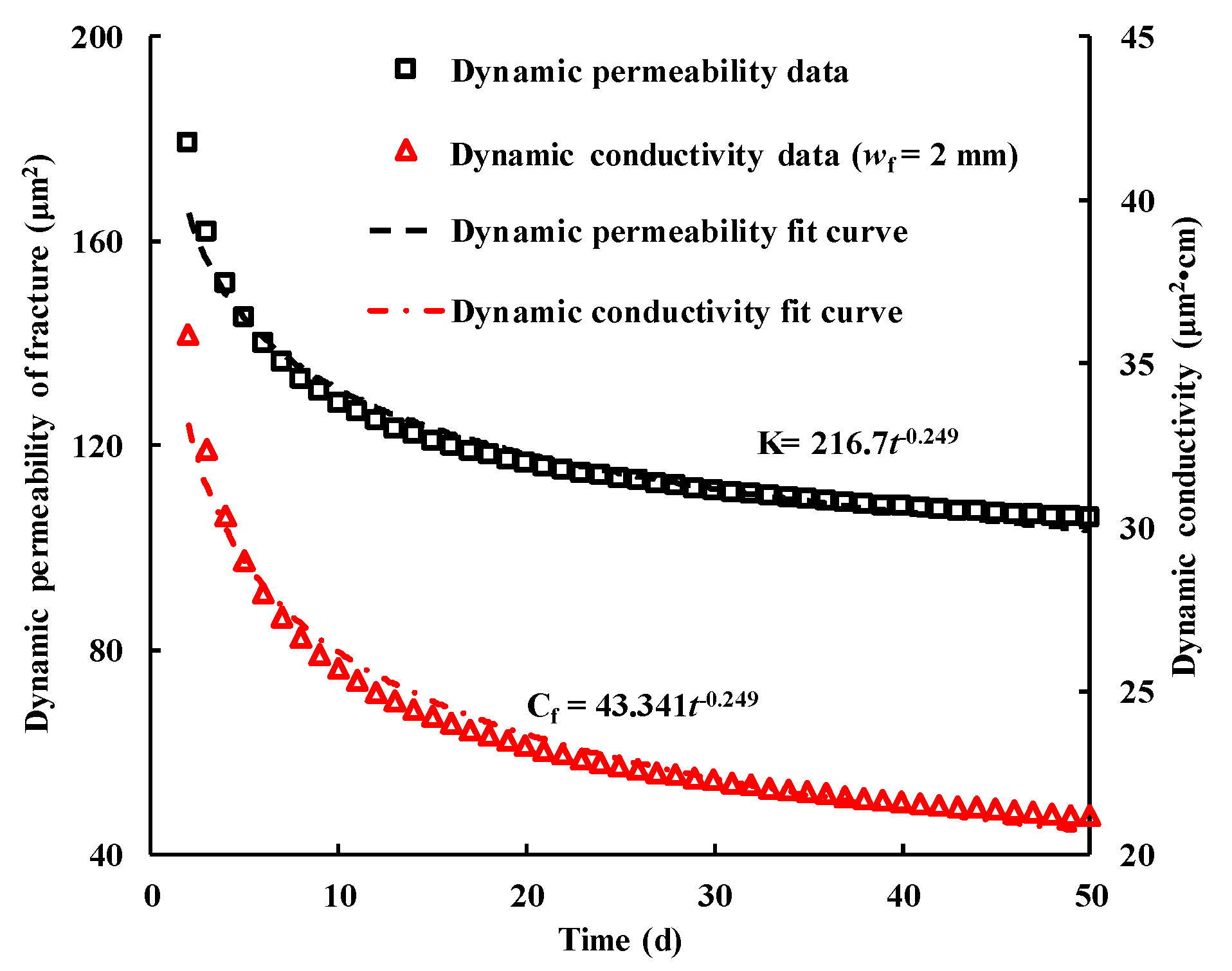
3.4. Dynamic Conductivity Evolution

To analyze the dynamic conductivity attenuation trend, ceramsite (30/50 mesh) is used as the proppant, the sand concentration is 5 kg/m², and the test fracturing fluid was slick water in conductivity test experiments. The experimental equipment is shown in Figure 2. And the dynamic conductivity test setup, including the test chamber and slate sample, is shown in Figure 3.

Figure 4 is generated from the experimental data; the fracture conductivity satisfies a power function relationship with the test time, as follows:

$$C_{\mathrm{f}}\left(t_{\mathrm{test}}\right)=k_{\mathrm{f}k}\left(t_{\mathrm{test}}\right)w_{\mathrm{f}k}=43.341{t_{\mathrm{test}}}^{-0.249}$$

(24)

3.5. Coupled Model

Combining Equations (10), (17), (22)–(24), one can obtain the coupled flow pressure drop squared equation from the reservoir to the k-th discrete node, which can be written as follows:

$$\begin{array}{l}\Delta p_k^2=\left\{\begin{array}{l}\Delta p_{\mathrm{r}k}^2+\Delta p_{\mathrm{sff}k-\mathrm{add}}^2+\Delta p_{\mathrm{f}k}^2 ,\left(t\le t_{\mathrm{refracture}}\right)\\ \Delta p_{\mathrm{r}k}^2+\Delta p_{\mathrm{sff}k-\mathrm{add}}^2+\Delta p_{\mathrm{f}k}^2 ,\left(t>t_{\mathrm{refracture}}\right)\end{array}\right.\\ =\left\{\begin{array}{l}{q}_{\mathrm{r}k}\left(F_k\left(x, y, z, t\right) +{\displaystyle \frac{2\mu p_{\mathrm{sc}}Z\mathrm{T}{b}_{\mathrm{s}}}{h\Delta x_{\mathrm{f}k}{T}_{\mathrm{sc}}{Z}_{\mathrm{sc}}{k}_{\mathrm{m}}}}{s}_{\mathrm{ff}k}\right) +{\displaystyle \frac{2{\mu }_g{p}_{\mathrm{sc}}\mathrm{ZT}}{K_{\mathrm{f}k}\left(t\right)w_{\mathrm{f}k}h{T}_{\mathrm{sc}}}}{\displaystyle \sum _{i=1}^{ns}\left( q_{\mathrm{r}i}{\displaystyle \sum _{j=1}^i\Delta x_{\mathrm{f}j}} \right)} ,\left(t\le t_{\mathrm{refracture}}\right)\\ q_{\mathrm{r}k}\left(F_k\left(x, y, z, t\right) +{\displaystyle \frac{2\mu p_{\mathrm{sc}}Z\mathrm{T}{b}_{\mathrm{s}}}{h\Delta x_{\mathrm{f}k}{T}_{\mathrm{sc}}{Z}_{\mathrm{sc}}{k}_{\mathrm{m}}}}{s}_{\mathrm{ff}k}\right) +{\displaystyle \frac{2{\mu }_g{p}_{\mathrm{sc}}\mathrm{ZT}}{K_{\mathrm{f}k}\left(t\right)w_{\mathrm{f}k}h{T}_{\mathrm{sc}}}}\left\{{\displaystyle \sum _{i=1}^j\left( q_{\mathrm{r}i}{\displaystyle \sum _{j=1}^i\Delta x_{\mathrm{f}j}} \right)+{\displaystyle \sum _{n=j+1}^{ns+m}\left[q_{\mathrm{r}n}\left({\displaystyle \sum _{i=1}^j\Delta x_{\mathrm{f}i}}\right)\right]}}\right\} ,\left(t>t_{\mathrm{refracture}}\right)\end{array}\right.\end{array}$$

(25)

The total production of the refractured vertical well is determined via discrete node flow rate superposition. Given a single fracture and refracture with ns + m nodes, we can obtain the following equation:

$$Q=\left\{\begin{array}{l}{\displaystyle \sum _{k=1}^{ns}{q}_{\mathrm{r}k}}\begin{array}{cc},& (t\le t_{\mathrm{refracture}})\end{array}\\ {\displaystyle \sum _{k=1}^{ns+m}{q}_{\mathrm{r}k}}\begin{array}{cc},& (t>t_{\mathrm{refracture}})\end{array}\end{array}\right.$$

(26)

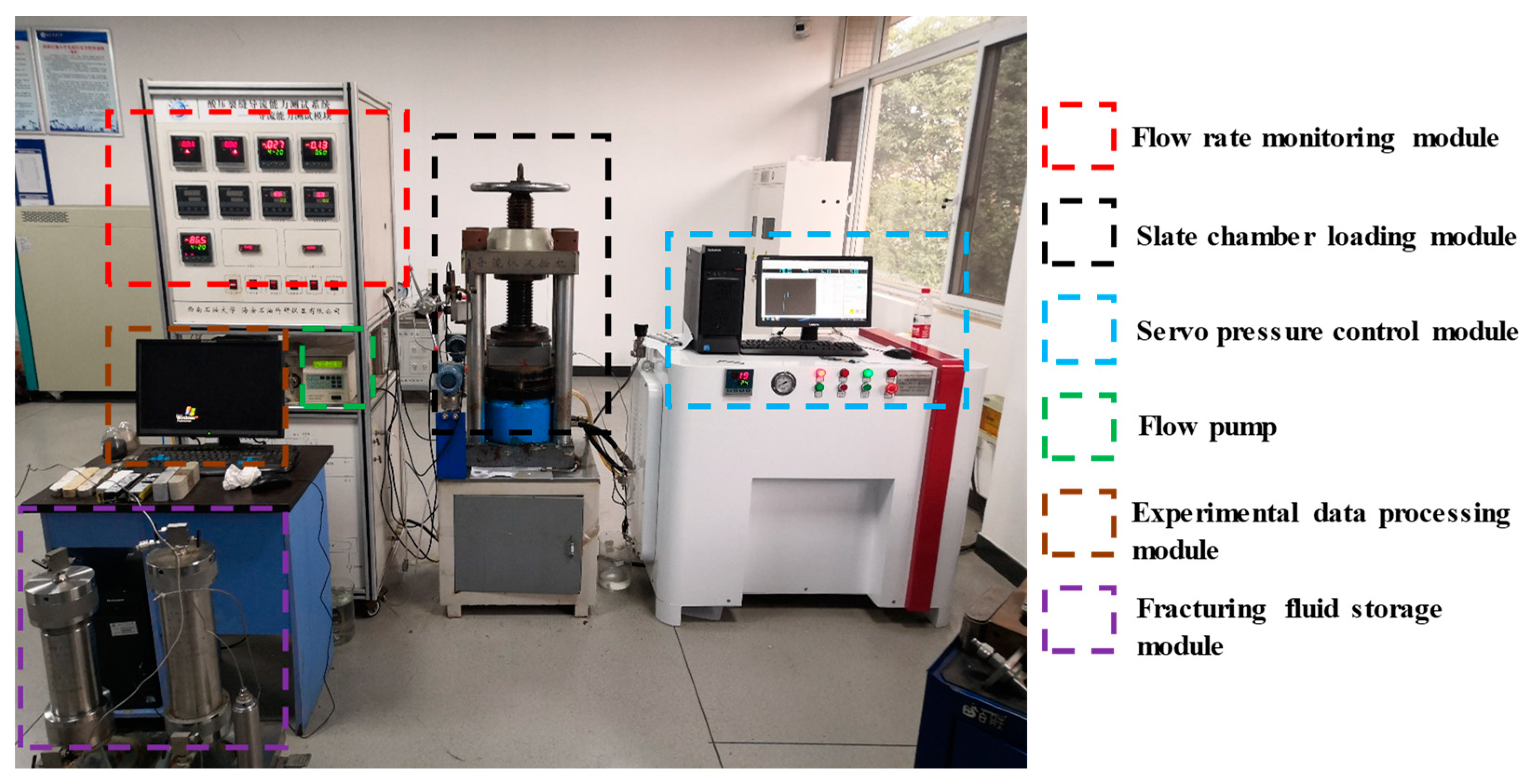
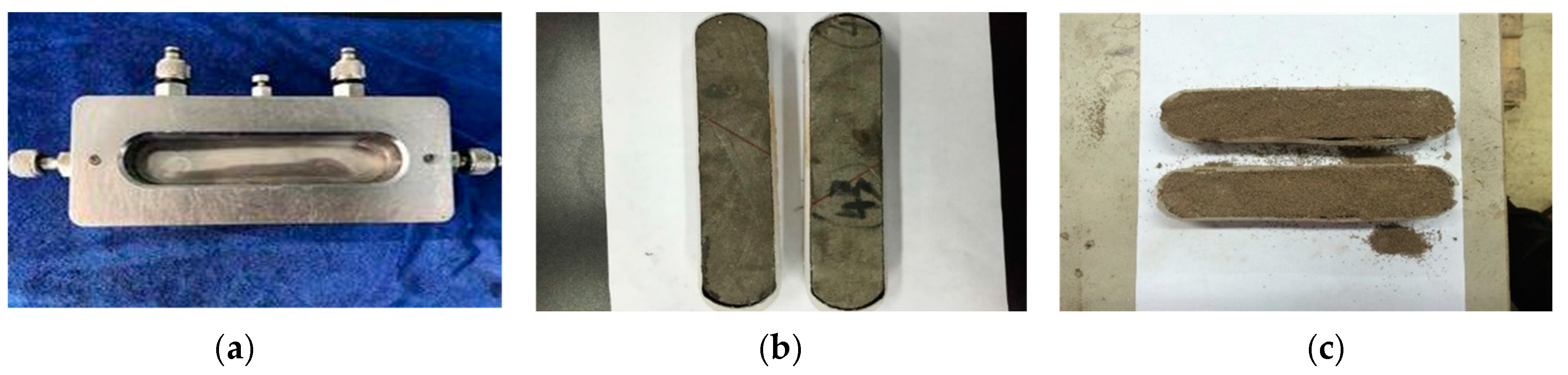
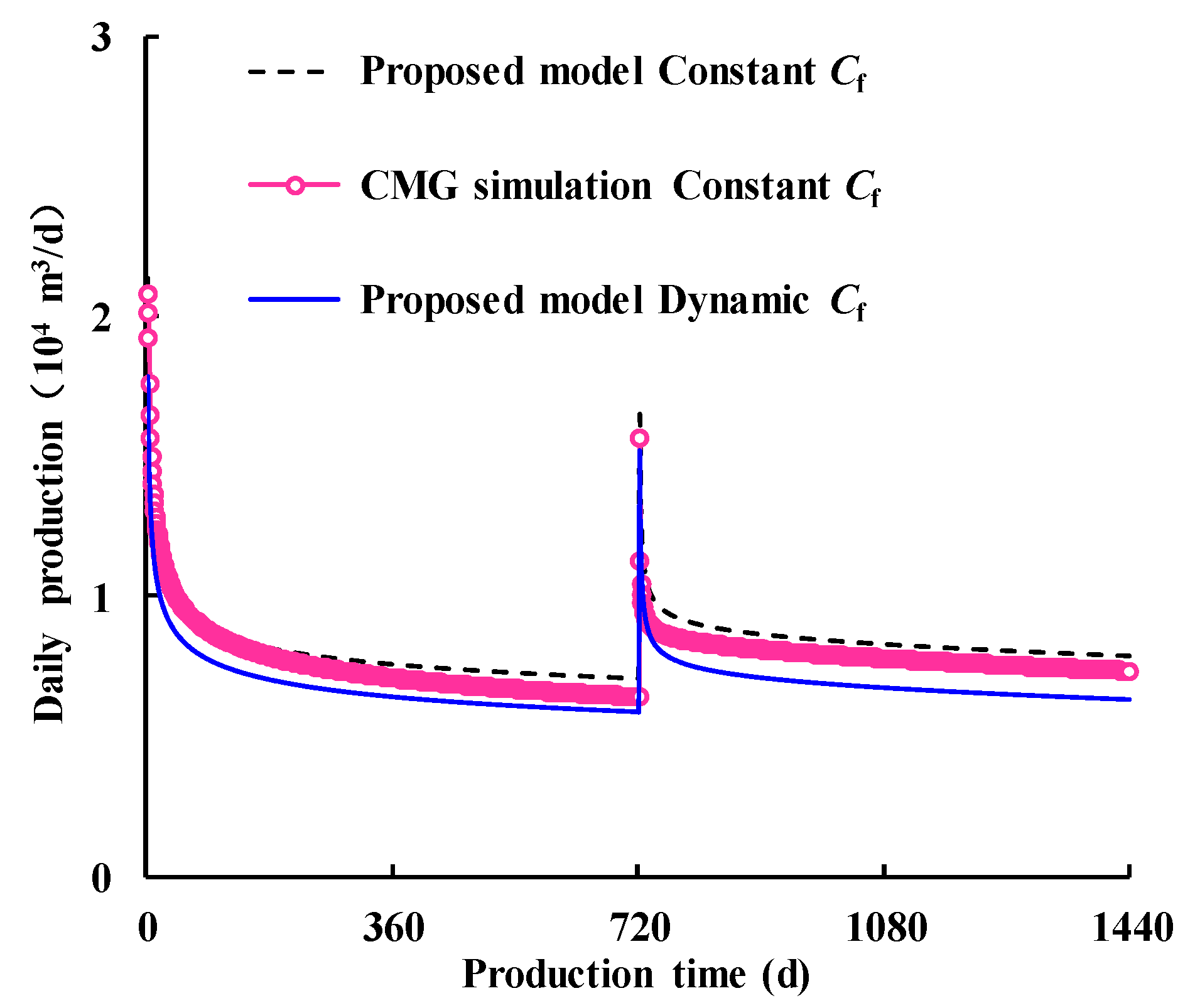
4. Model Solution and Verification

4.1. The Solution Method

The matrix form of the linear equation system of the semi-analytical mathematical model for refractured vertical wells in tight gas reservoirs is given in detail in Appendix B, and a computer algorithm is designed to solve this mathematical model. A flow chart is shown in Figure 5.

4.2. Model Verification

The numerical simulation model of a vertical fractured well is constructed in CMG software for 2022.30 version to verify the reliability of the proposed model, as shown in Figure 6a. Considering constant-BHP constraints (20 MPa), we set the grid size to 8 m × 8 m and define 100 meshes along the I and J directions and 1 layer along the K direction with a thickness of 20 m. The refracture job is set 720 days after the initial fracture, and the refracture mesh configuration was refined as shown in Figure 6b. The fracture conductivity, fracture length, and width are consistent with the values provided in

Table 1. Reservoir properties for simulation.

Parameter	Unit	Value	Parameter	Unit	Value
Reservoir length	m	800	Segments of the initial fracture	—	16
Reservoir width	m	800	Segments of the refracture	—	12
Reservoir thickness	m	20	Fracture width	mm	2
Reservoir permeability	10−3 μm2	0.1	Gas deviation factor	—	0.89
Reservoir porosity	—	0.16	Gas relative density	—	0.6
Initial reservoir pressure	MPa	40	Gas viscosity at 341 K	mPa·s	0.009
Bottom-hole pressure	MPa	20	Gas constant	J/(mol·K)	8.314
Conductivity	D•cm	6	Gas density at 341 K	kg/m3	0.655
Initial fracture length	m	120	Irreducible water saturation	%	10
Refracture fracture length	m	120	Compression factor	MPa−1	0.035

.

Figure 7 compares the results of CMG software and the proposed model. When the constant conductivity of 6 D•cm is applied, the proposed model is consistent with the CMG simulation results, which verifies the accuracy of the proposed model. When dynamic conductivity is applied in the proposed model, the daily production is 10% lower than that of constant conductivity, which implies that the fracture conductivity impairment cannot be ignored.

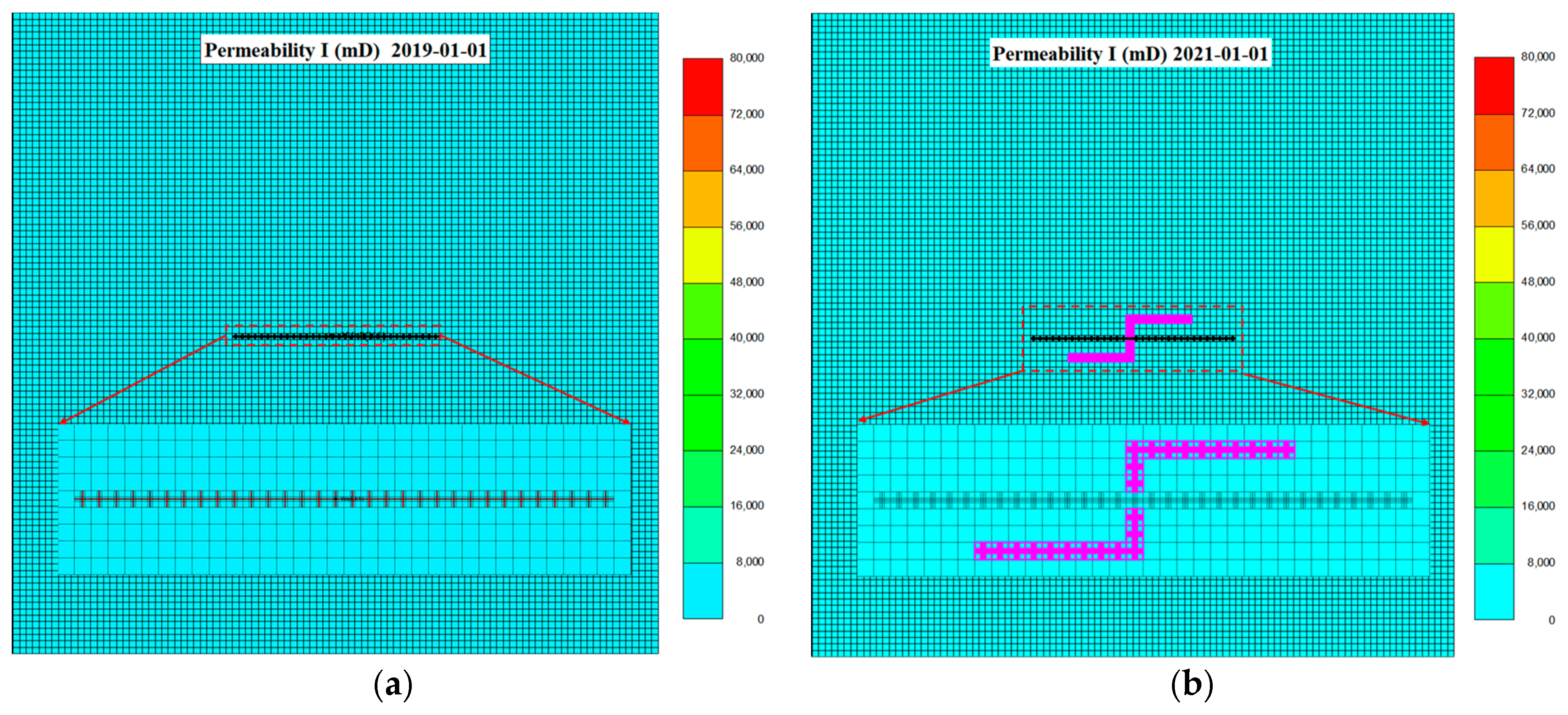
5. Application: Tight Gas Reservoir in Linxing Field

5.1. Reservoir Characteristics

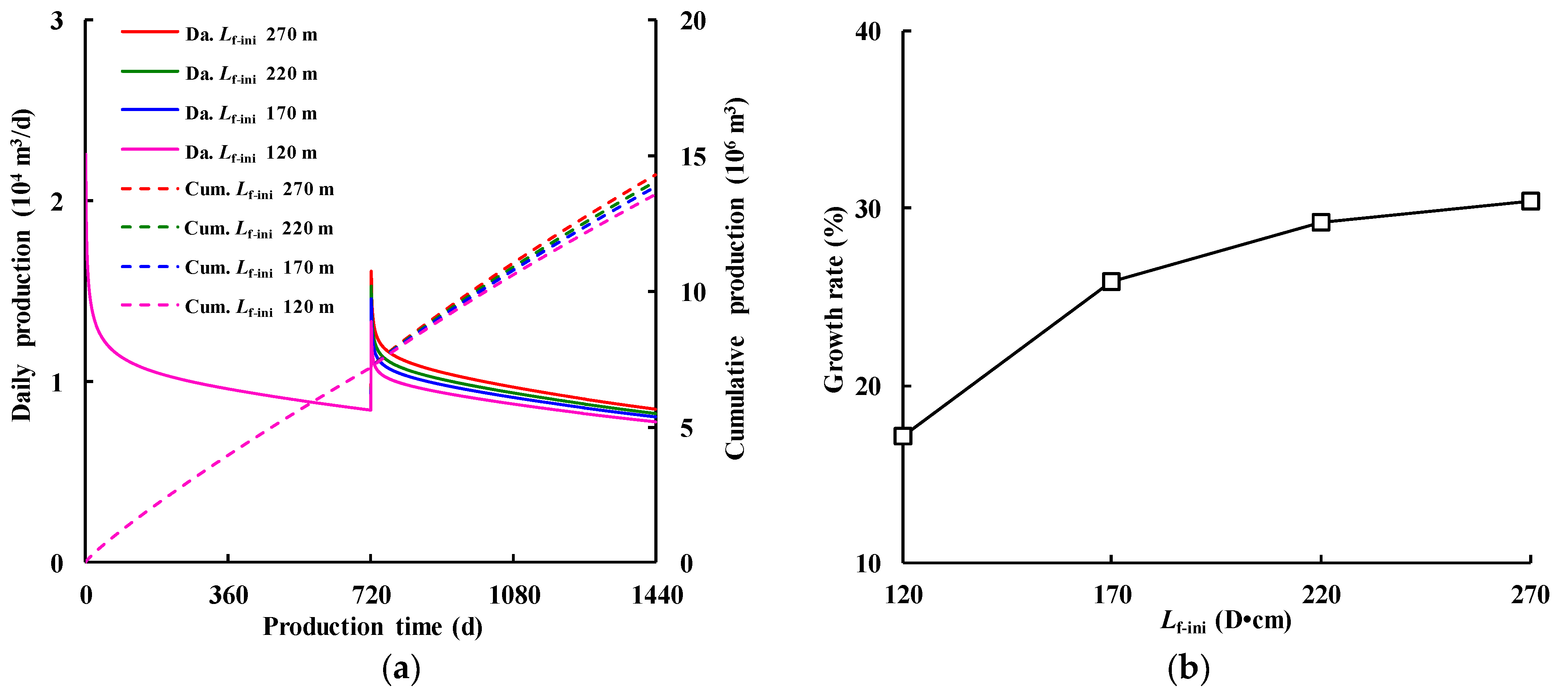
Linxing tight gas field located in western Sichuan basin, the thickness of the main production layers is 20 m, porosity is 7.2~23.4%, and permeability is 0.05 × 10⁻³~0.22 × 10⁻³ μm². The daily gas production of most wells steeply attenuates from 3.0~5.0 ×10⁴ m³/d to less than 1.0 × 10⁴ m³/d within two years. Therefore, the performance of the old well urgently needs to be restored by a refracture job. The basic parameter values and the reservoir properties are listed in Table 1.

5.2. Analysis

In this section, the refractured well flow characteristics are analyzed by the proposed model and design optimization of well(X1) in Linxing tight gas field. Subsequently, the hydraulic fracture parameters (i.e., fracture length and conductivity, stimulated fracture permeability, and width) can be further determined.

Figure 8 shows the refracturing timing impact on the well performance. Further, define the growth rate $GR=\left(Q_{\mathrm{refracture}}-Q_{\mathrm{non}-\mathrm{refracture}}\right)/Q_{\mathrm{non}-\mathrm{refracture}}\times 100\%, t>t_{\mathrm{refracture}}$ to describe the impact on each scenario. One can find that the earlier the refracturing timing, the higher the daily output at the initial stage (Figure 8a). This is due to the conductivity decay over production time (Equation (24)). Figure 8b shows that, throughout the refracture stage, the GR approaches 28% in the 720 d scenario and decreases with the delay of the fracturing timing. Consequently, to ensure effective recovery and enhance production, a refracture job should be carried out as soon as possible when daily production is lower than the desired value.

Figure 9 shows the initial fracture conductivity impact on the well performance. Figure 9a indicates both the initial daily production and cumulative production are positively correlated with conductivity. However, the gas production is only slightly improved while the C_f-ini is larger than 6 D•cm. Figure 9b shows the GR tends to flatten as C_f-ini increases, C_f-ini further increased from 8 to 10 D•cm, and the GR is merely enhanced by 2%. There are two reasons for this phenomenon. First, the fluid around the initial fractures has been recovered. Second, the production capacity of the tight sandstone reservoirs with low permeability is confined, and appropriate lower conductivity can satisfy the production requirements [32,42]. Therefore, the optimal C_f-ini is 8 D•cm is recommended in this field case.

Figure 10 shows the refracture conductivity impact on the well performance. Similar to C_f-ini scenarios, the production enhancement positively correlated with C_f-refrac, and exists at inflection point 8 D•cm, Figure 10a,b. Consequently, the optimal C_f-ref is 8~10 D•cm.

Figure 11 shows the extended initial fracture length impact on the well performance. The essence of the refracture job is to create new fractures to connect undeveloped reservoirs. As shown in Figure 11a,b, the daily production increased significantly with the L_f-ini increase from 120~270 m. Hence, it is essential to extend the initial fracture length as much as possible under engineering conditions. And the optimal L_f-ini is 220 m in this field case.

Figure 12 shows the refracture length impact on the well performance. Figure 12a presents the refracture production positively correlated with L_f-ref. The growth rates flatten as refracture length increases, and the optimal L_f-ref is 100~150 m, as shown in Figure 12b.

The negative skin factors s_ffk and b_s are introduced to treat the effects of the c omplex fracture networks. k_s/k_m = 1 indicates that refracturing does not produce a secondary fracture network, while k_s/k_m > 1 indicates that the permeability in fracture networks is enhanced. The b_s represents the stimulated width produced from refracture construction.

Figure 13 shows the value of k_s/k_m effect on the well performance. Daily production and growth rate increase with the value of k_s/k_m (Figure 13a,b). With k_s/k_m increasing from 1 to 10, the growth rate increases sharply from 25% to 33%, and with further increases to 50 and 100, the GR can almost be ignored. The optimal value of k_s/k_m is 10.

Figure 14a,b present the stimulated width d_s effect on refracture well performance. It shows that b_s can dramatically increase the initial and overall production of fractured wells. When b_s varies from 1 m to 4 m, the growth rate increases from 22% to 60%. In summary, compared to fracture length, conductivity, and fracture network permeability, further producing larger stimulated width b_s is vital to enhancing production for the refracture job.

5.3. Optimization

This section illustrates a field application for the proposed model in a vertical fractured gas well(X1) with fast production decline. The depth of well(X1) is 2100 m. The objective of the refracture job is to create new fractures with stimulated volume and to restore and maintain the conductivity. To establish reasonable simulation parameters for optimization analysis, the history match of well(X1) is completed based on production data, and the refracture well performance can be predicted, as shown in Figure 15.

The fitting result shows the fracture length is approaching 120 m, and the conductivity is almost reduced to 0, causing the hydraulic fracture to almost close. Based on the above-mentioned, selecting the fracture length and conductivity, secondary fracture permeability, and width to conduct the orthogonal tests L₁₆(4⁶), the experimental program is shown in

Table 2. Simulation schemes L₁₆(4⁶).

No.	Lf-ini (m)	Lf-ref (m)	Cf-ini (D•cm)	Cf-ref (D•cm)	ks (mD)	bs (m)	No.	Lf-ini (m)	Lf-ref (m)	Cf-ini (D•cm)	Cf-ref (D•cm)	ks (mD)	bs (m)
Test 1	120	50	8	6	1	3	Test 9	220	150	10	4	10	1
Test 2	120	100	10	8	5	4	Test 10	220	200	4	6	0.1	2
Test 3	120	150	4	10	10	1	Test 11	220	50	6	8	1	3
Test 4	120	200	6	4	0.1	2	Test 12	220	100	8	10	5	4
Test 5	170	100	4	8	0.1	4	Test 13	270	200	6	10	5	2
Test 6	170	150	6	10	1	1	Test 14	270	50	8	4	10	3
Test 7	170	200	8	4	5	2	Test 15	270	100	10	6	1	4
Test 8	170	50	10	6	10	3	Test 16	270	150	4	8	0.1	1

, and the optimal hydraulic fracture parameter combination can be determined. Therefore, it can better guide the refracturing job in the field.

Based on the simulation results, shown in Figure 16a,b, of the proposed model in this paper, the optimal hydraulic fracture parameter combination can be obtained: the initial fracture length of 220 m, create refracture length of 100 m, restore initial fracture conductivity of 8 D•cm, maintain refracture conductivity of 10 D•cm, fracture network permeability of 5 mD and width of 4 m, and extreme analysis shows that the important level is ranked as b_s > L_f-ini > L_f-ref > C_f-ini > k_s > C_f-ref.

The optimal hydraulic fracture parameters are used to calculate the construction parameters (pad fluid 340 m³, carrying fluid 600 m³, displacement fluid 40 m³, treatment volume 10 m³/min, temporary plugging agent 54 kg, proppant 1000 kg) for the well(X1) refracture job using commercial software. Finally, after refracturing construction, well(X1) obtained production of 1.5 × 10⁴ m³/d in the early stage, which recovered to more than 90% of the initial fracture job.

Figure 17 illustrates that the refracture job extends the initial fracture and creates the refracture, greatly connecting undeveloped reservoirs. During gas production, the pressure spread at 1440 d is much larger than before the refracture job.

6. Conclusions

A semi-analytical model and the hydraulic fracture optimization method of the refractured well in a tight sand gas reservoir are constructed using the Newman integral method with Green’s function, which can be applied to fracture network properties and considers the dynamic conductivity. Verification by commercial software reveals that a high agreement is attained; subsequently, the optimizations for the refracture design are applied in well(X1) in Linxing field, the sensitivity analysis and hydraulic fracture parameter optimization results are as follows:

(1)

To ensure effective recovery and enhance production, the refracture job should be carried out as soon as possible when daily production is lower than the desired value;

(2)

Restoring the initial fractures (C_f-ini) and constructing the refractures (C_f-ref), conductivity can increase productivity, which increases over 8 D•cm; the production growth rate just obtains a slight improvement; both optimal C_f-ini and C_f-ref are 8 D•cm, which is recommended in this field case;

(3)

Extending the initial fractures and creating the refractures means more reservoirs can be developed, and the daily production significantly increases with L_f-ini increasing from 120~270 m and L_f-ref increasing from 100~150 m. Hence, it is essential to extend the length of the initial fracture as much as possible under engineering conditions; the optimal L_f-ini is 220 m and L_f-ref is 150 in this field case;

(4)

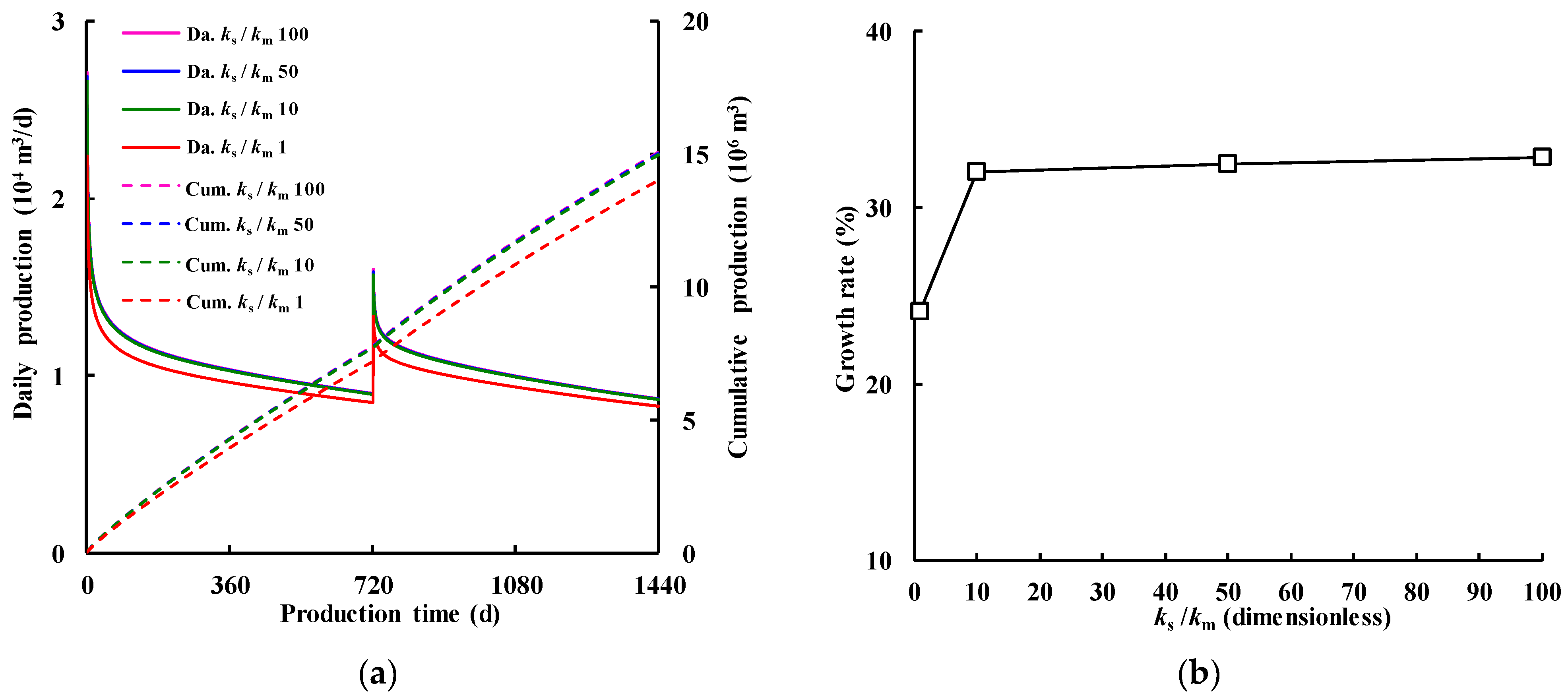
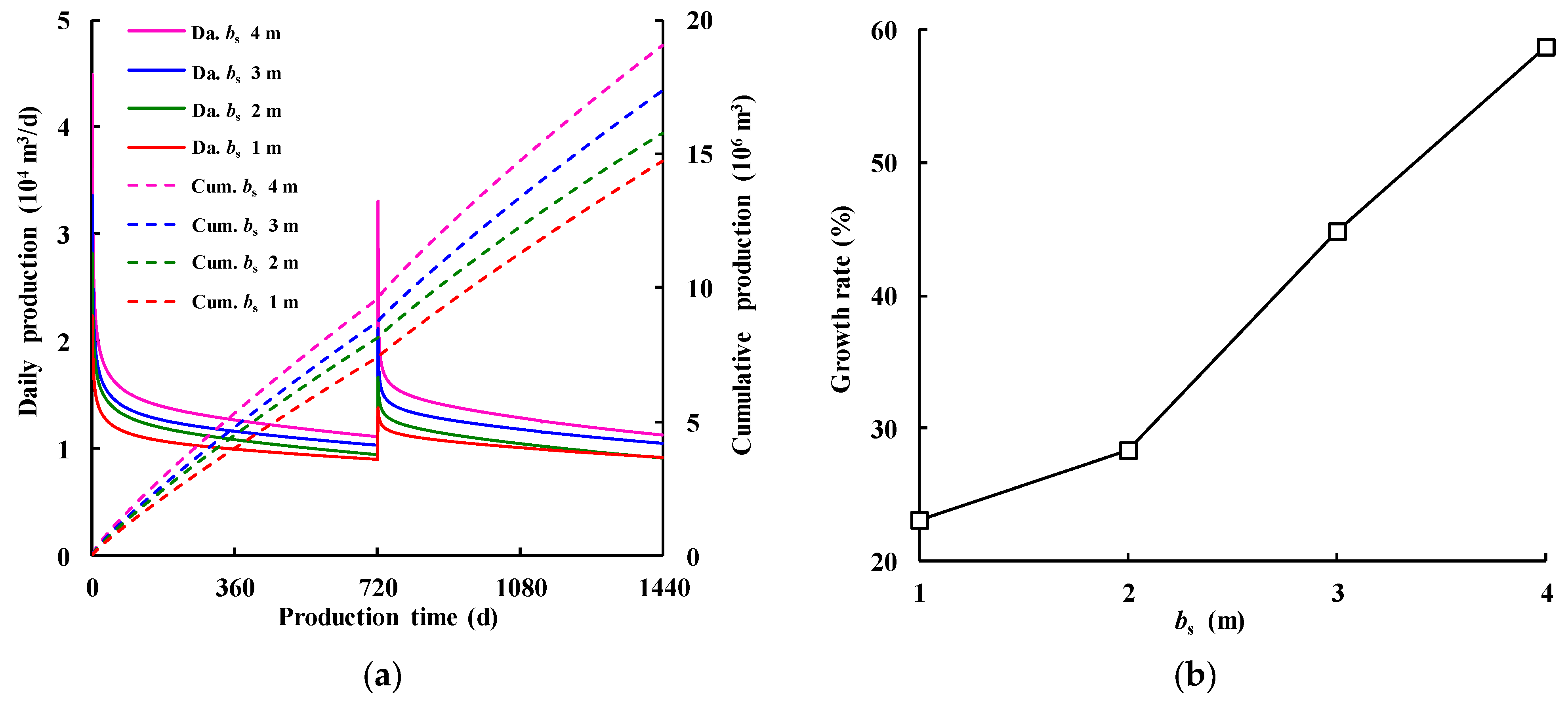
In a tight sand gas reservoir, the k_s/k_m = 10 can obviously increase production, but for enlarged fracture networks, the permeability k_s does not contribute to well performance. Conversely, further producing larger stimulated width b_s is vital to enhance production for the refracture job;

(5)

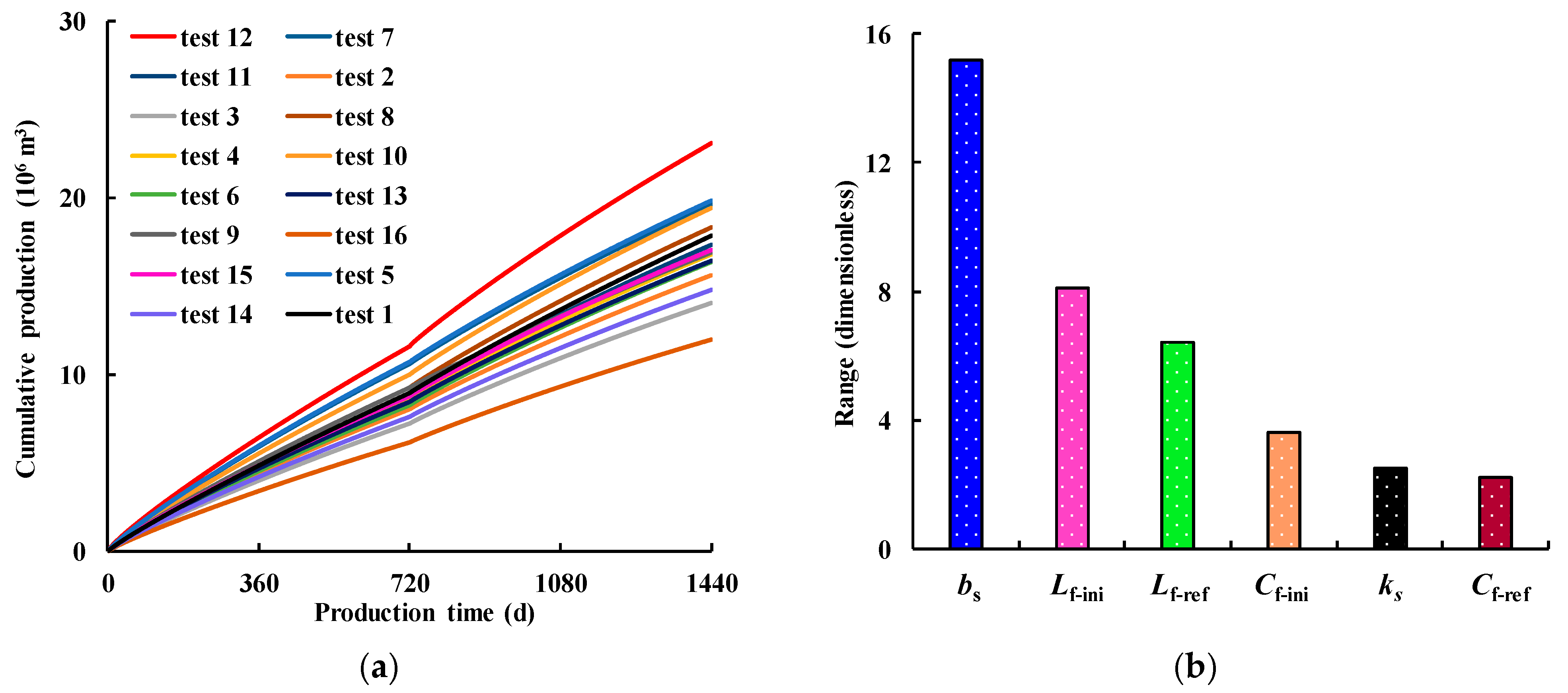
The orthogonal experiments indicate that the optimal hydraulic fracture parameter combinations with important rank for well(X1) are: d_s (4 m) > L_f-ini (220 m) > L_f-ref (100 m) > C_f-ini (8 D•cm) > k_s (5 mD) > C_f-ref (10 D•cm). Based on the optimal design, the productivity of well(X1) recovery is more than 90% after the refracture job.

References

1. Holditch, S.A. Tight Gas Sands. J. Pet. Technol. 2006, 58, 86–93. [Google Scholar] [CrossRef]
2. Guo, S.; Li, Y.; Chen, T.; Zheng, D.; Du, J.; Bu, Y.; Zhou, A.; Pang, X.; Liu, H. Controlling the hydration rate of alkali-activated slag by the slow release of NaOH. Geoenergy Sci. Eng. 2023, 228, 211960. [Google Scholar] [CrossRef]
3. Zeng, F.; Yang, B.; Guo, J.; Chen, Z.; Xiang, J. Experimental and Modeling Investigation of Fracture Initiation from Open-Hole Horizontal Wells in Permeable Formations. Rock Mech. Rock Eng. 2019, 52, 1133–1148. [Google Scholar] [CrossRef]
4. Wang, J.Y.; Holditch, S.; Mcvay, D. Modeling fracture-fluid cleanup in tight-gas wells. SPE J. 2010, 15, 783–793. [Google Scholar] [CrossRef]
5. Jacobs, T. Renewing Mature Shale Wells through Refracturing. J. Pet. Technol. 2014, 66, 52–60. [Google Scholar] [CrossRef]
6. Snyder, D.; Seale, R.A. Optimization of Completions in Unconventional Reservoirs for Ultimate Recovery-Case Studies. In Proceedings of the SPE EUROPEC/EAGE Annual Conference and Exhibition, Vienna, Austria, 23–27 May 2011; Society of Petroleum Engineers: Richardson, TX, USA. [Google Scholar]
7. Cramer, D.D. Fracture Skin: A Primary Cause of Stimulation Ineffectivenessas in Gas Wells. In Proceedings of the SPE Annual Technical Conference and Exhibition, San Antonio, TX, USA, 9–11 October 2005; Society of Petroleum Engineers: Richardson, TX, USA. [Google Scholar]
8. Ding, D.Y.; Langouët, H.; Jeannin, L. Simulation of fracturing-induced formation damage and gas production from fractured wells in tight gas reservoirs. SPE Prod. Oper. 2013, 28, 246–258. [Google Scholar] [CrossRef]
9. Wen, Q.; Zhang, S.; Wang, L.; Liu, Y.; Li, X. The effect of proppant embedment upon the long-term conductivity of fractures. J. Pet. Sci. Eng. 2007, 55, 221–227. [Google Scholar] [CrossRef]
10. Barree, R.D.; Miskimins, J.L.; Svatek, K.J. Reservoir and completion considerations for the refracturing of horizontal wells. SPE Prod. Oper. 2018, 33, 1–11. [Google Scholar] [CrossRef]
11. Shah, M.; Shah, S.; Sircar, A. A comprehensive overview on recent developments in refracturing technique for shale gas reservoirs. J. Nat. Gas Sci. Eng. 2017, 46, 350–364. [Google Scholar] [CrossRef]
12. Akbari, M.; Ameri, M.J.; Kharazmi, S.; Motamedi, Y.; Pournik, M. New correlations to predict fracture conductivity based on the rock strength. J. Pet. Sci. Eng. 2017, 152, 416–426. [Google Scholar] [CrossRef]
13. Shamsi, M.M.M.; Nia, S.F.; Jessen, K. Dynamic conductivity of proppant-filled fractures. J. Pet. Sci. Eng. 2017, 151, 183–193. [Google Scholar] [CrossRef]
14. Lindsay, G.J.; White, D.J.; Miller, G.A.; Baihly, J.D.; Sinosic, B. Understanding the applicability and economic viability of refracturing horizontal wells in unconventional plays. In Proceedings of the SPE Hydraulic Fracturing Technology Conference, The Woodlands, TX, USA, 9–11 February 2016; Society of Petroleum Engineers: Richardson, TX, USA. [Google Scholar]
15. Teng, B.; Li, H.A. A Semianalytical Model for Evaluating the Performance of a Refractured Vertical Well with an Orthogonal Refracture. SPE J. 2019, 24, 891–911. [Google Scholar] [CrossRef]
16. Luo, L.; Cheng, S.; Lee, J. Characterization of refracture orientation in poorly propped fractured wells by pressure transient analysis: Model, pitfall, and application. J. Nat. Gas Sci. Eng. 2020, 79, 103332. [Google Scholar] [CrossRef]
17. Sophie, S.Y.; Sharma, M.M. A new method to calculate slurry distribution among multiple fractures during fracturing and refracturing. J. Pet. Sci. Eng. 2018, 170, 304–314. [Google Scholar]
18. Li, W.; Zhao, H.; Pu, H.; Zhang, Y.; Wang, L.; Zhang, L.; Sun, X. Study on the mechanisms of refracturing technology featuring temporary plug for fracturing fluid diversion in tight sandstone reservoirs. Energy Sci. Eng. 2019, 7, 88–97. [Google Scholar] [CrossRef]
19. Zeng, F.; Guo, J. Optimized design and use of induced complex fractures in horizontal wellbores of tight gas reservoirs. Rock Mech. Rock Eng. 2016, 49, 1411–1423. [Google Scholar] [CrossRef]
20. Zeng, F.; Zhang, Y.; Guo, J.; Zhang, Q.; Chen, Z.; Xiang, J.; Zheng, Y. Optimized completion design for triggering a fracture network to enhance horizontal shale well production. J. Pet. Sci. Eng. 2020, 190, 107043. [Google Scholar] [CrossRef]
21. Dusterhoft, R.G.; East, L.E.; Soliman, M.Y. Fracturing a Stress-Altered Subterranean Formation. U.S. Patent 8,210,257, 3 July 2012. [Google Scholar]
22. Mohaghegh, S.; Mohamad, K.; Popa, A.; Ameri, S.; Wood, D. Performance drivers in restimulation of gas-storage wells. SPE Reserv. Eval. Eng. 2001, 4, 536–542. [Google Scholar] [CrossRef]
23. Roussel, N.P.; Sharma, M.M. Selecting candidate wells for refracturing using production data. SPE Prod. Oper. 2013, 28, 36–45. [Google Scholar] [CrossRef]
24. Warpinski, N.R.; Branagan, P.T. Altered-stress fracturing. J. Pet. Technol. 1989, 41, 990–997. [Google Scholar] [CrossRef]
25. Roussel, N.P.; Sharma, M.M. Quantifying transient effects in altered-stress refracturing of vertical wells. SPE J. 2010, 15, 770–782. [Google Scholar] [CrossRef]
26. Oruganti, Y.; Mittal, R.; McBurney, C.J.; Rodriguez, A. Re-fracturing in eagle ford and Bakken to increase reserves and generate incremental NPV: Field study. In Proceedings of the SPE Hydraulic Fracturing Technology Conference, The Woodlands, TX, USA, 3–5 February 2015; Society of Petroleum Engineers: Richardson, TX, USA. [Google Scholar]
27. Teng, B.; Li, H.A. A semi-analytical model for characterizing the fluid transient flow of reoriented refractures. J. Pet. Sci. Eng. 2019, 177, 921–940. [Google Scholar] [CrossRef]
28. Zhou, W.; Banerjee, R.; Poe, B.D.; Spath, J.; Thambynayagam, M. Semianalytical production simulation of complex hydraulic-fracture networks. SPE J. 2013, 19, 6–18. [Google Scholar] [CrossRef]
29. Hazlett, R.D.; Babu, D.K. Discrete wellbore and fracture productivity modeling for unconventional wells and unconventional reservoirs. SPE J. 2014, 19, 19–33. [Google Scholar] [CrossRef]
30. Ostojic, J.; Rezaee, R.; Bahrami, H. Production performance of hydraulic fractures in tight gas sands, a numerical simulation approach. J. Pet. Sci. Eng. 2012, 88, 75–81. [Google Scholar] [CrossRef]
31. Suzuki, K. Influence of wellbore hydraulics on horizontal well pressure transient behavior. SPE Form. Eval. 1997, 12, 175–181. [Google Scholar] [CrossRef]
32. Yao, S.; Zeng, F.; Liu, H.; Zhao, G. A semi-analytical model for multi-stage fractured horizontal wells. J. Hydrol. 2013, 507, 201–212. [Google Scholar] [CrossRef]
33. Pan, Y.; Kamal, M.M.; Kikani, J. Field applications of a semianalytical model of multilateral wells in multilayer reservoirs. SPE Reserv. Eval. Eng. 2010, 13, 861–872. [Google Scholar] [CrossRef]
34. He, Y.; Cheng, S.; Li, S.; Huang, Y.; Qin, J.; Hu, L.; Yu, H. A semianalytical methodology to diagnose the locations of underperforming hydraulic fractures through pressure-transient analysis in tight gas reservoir. SPE J. 2017, 22, 924–939. [Google Scholar] [CrossRef]
35. Yang, R.; Huang, Z.; Li, G.; Yu, W.; Sepehrnoori, K.; Lashgari, H.R.; Tian, S.; Song, X.; Sheng, M. A semianalytical approach to model two-phase flowback of shale-gas wells with complex-fracture-network geometries. SPE J. 2017, 22, 1808–1833. [Google Scholar] [CrossRef]
36. He, J.; Okere, C.J.; Su, G.; Hu, P.; Zhang, L.; Xiong, W.; Li, Z. Formation damage mitigation mechanism for coalbed methane wells via refracturing with fuzzy-ball fluid as temporary blocking agents. J. Nat. Gas Sci. Eng. 2021, 90, 103956. [Google Scholar] [CrossRef]
37. Horne, R. The Fenske conservation method for pressure transient solutions with storage. Soc. Pet. Eng. J. 1985, 25, 437–444. [Google Scholar] [CrossRef]
38. Yu, W.; Wu, K.; Sepehrnoori, K. A Semianalytical Model for Production Simulation from Nonplanar Hydraulic-Fracture Geometry in Tight Oil Reservoirs. SPE J. 2016, 21, 1028–1040. [Google Scholar] [CrossRef]
39. Lin, J.; Zhu, D. Predicting Well Performance in Complex Fracture Systems by Slab Source Method. In Proceedings of the SPE Hydraulic Fracturing Technology Conference and Exhibition, The Woodlands, TX, USA, 6–8 February 2012. [Google Scholar]
40. Lin, J.; Zhu, D. Modeling well performance for fractured horizontal gas wells. J. Nat. Gas Sci. Eng. 2014, 18, 180–193. [Google Scholar] [CrossRef]
41. Clarkson, C.R. Production data analysis of unconventional gas wells: Review of theory and best practices. Int. J. Coal Geol. 2013, 109–110, 101–146. [Google Scholar] [CrossRef]
42. Zeng, J.; Wang, X.; Guo, J.C. Composite linear flow model for multi-fractured horizontal wells in heterogeneous shale reservoir. J. Nat. Gas Sci. Eng. 2017, 38, 527–548. [Google Scholar] [CrossRef]
43. Lian, P.; Cheng, L.; Cui, J. A new computation model of fractured horizontal well coupling with reservoir. Int. J. Numer. Methods Fluids 2011, 67, 1047–1056. [Google Scholar] [CrossRef]
44. Cinco, L.; Samaniego, V.; Dominguez, A. Transient pressure behavior for a well with a finite-conductivity vertical fracture. Soc. Pet. Eng. J. 1978, 18, 253–264. [Google Scholar] [CrossRef]
45. Van Everdingen, A.F. The Skin Effect and Its Influence on the Productive Capacity of a Well. J. Pet. Technol. 1953, 5, 171–176. [Google Scholar] [CrossRef]
46. Tayong, R.; Alhubail, M.M.; Maulianda, B.; Barati, R. Simulating yield stress variation along hydraulic fracture face enhances polymer cleanup modeling in tight gas reservoirs. J. Nat. Gas Sci. Eng. 2019, 65, 32–44. [Google Scholar] [CrossRef]
47. Kuchuk, F.J.; Goode, P.A.; Wilkinson, D.J.; Thambynayagam, R.K.M. Pressure-Transient Behavior of Horizontal Wells with and without Gas Cap or Aquifer. SPE Form. Eval. 1991, 6, 86–94. [Google Scholar] [CrossRef]
48. Zhang, Z.; Guo, J.; Liang, H.; Liu, Y. Numerical simulation of skin factors for perforated wells with crushed zone and drilling-fluid damage in tight gas reservoirs. J. Nat. Gas Sci. Eng. 2021, 90, 103907. [Google Scholar] [CrossRef]
49. Zeng, F.H.; Cheng, X.Z.; Guo, J.C.; Long, C.; Ke, Y. A New Model to Predict the Unsteady Production of Fractured Horizontal Wells (Model Baharu untuk Meramalkan Pengeluaran tak Menentu Telaga Mendatar yang Retak). Sains Malays. 2016, 45, 1579–1587. [Google Scholar]
Figure 1. Schematic of the refracture and discretization segments.
Processes 12 02033 g001
Figure 2. Experimental device and schematic diagram of the component modules.
Processes 12 02033 g002
Figure 3. Images of the slate test sample and holder. (a) Slate holder; (b) Slate before the test; (c) Slate after the test.
Processes 12 02033 g003
Figure 4. Schematic diagram of the experimental data.
Processes 12 02033 g004
Figure 5. Solution program flowchart of the semi-analytical model.
Processes 12 02033 g005
Figure 6. Schematics of the initial CMG simulation model and refracture model. (a) Initial fracture; (b) Refracture.
Processes 12 02033 g006
Figure 7. Simulation results of the proposed model versus commercial software.
Processes 12 02033 g007
Figure 8. Daily and cumulative production versus different refracturing timing scenarios. (a) Impact of the refracture timing; (b) Growth rate.
Processes 12 02033 g008
Figure 9. Daily and cumulative production versus different initial fracture conductivity scenarios. (a) Impact of the initial fracture conductivity; (b) Growth rate.
Processes 12 02033 g009
Figure 10. Daily and cumulative gas production versus different refracture conductivity scenarios. (a) Impact of the refracture conductivity; (b) Growth rate.
Processes 12 02033 g010
Figure 11. Daily and cumulative production versus different extended initial fracture length scenarios. (a) Impact of the extended initial fracture length; (b) Growth rate.
Processes 12 02033 g011
Figure 12. Daily and cumulative production versus different refracture length scenarios. (a) Impact of the refracture length; (b) Growth rate.
Processes 12 02033 g012
Figure 13. Daily and cumulative production for the different ks/km scenarios. (a) Impact of the fracture network permeability; (b) Growth rate.
Processes 12 02033 g013
Figure 14. Daily and cumulative production for the different bs scenarios. (a) Impact of the fracture network width; (b) Growth rate.
Processes 12 02033 g014
Figure 15. History match and refracturing production prediction to well(X1).
Processes 12 02033 g015
Figure 16. Orthogonal experiment results and fracture parameter importance range based on 4-year cumulative gas production. (a) 4-year cumulative gas production; (b) fracture parameter importance range.
Processes 12 02033 g016
Figure 17. Pressure diffusion characteristics before and after refracturing based on optimal design.
Processes 12 02033 g017