Effect of Heat-Treatment Process on Magnetic Characteristics of Grain-Oriented Electrical Steel

Abstract

This paper explores the effects and impacts of the metallurgical process of quenching on grain-oriented strips of electrical steel. Experimental findings reveal that quenching resulted in increased hardness and an increased Young’s modulus. An analysis of the material structure post-quenching indicates significant alterations in grain spacing and reduced height differences between grains. However, the magnetic properties of the steel deteriorated following quenching.

1. Introduction

In response to the rapid developments and high demand for soft magnetic electrical steels, this article examines the effects of quenching, a well-known metallurgical process used for hardening steel. The objective is to determine whether it is possible to create an electrical steel material that combines the hardness of quenched steel with the magnetic properties of grain-oriented electrical steel, suitable for applications in which a power transformer core is subjected to significant mechanical stress, and whether this can be obtained with the thermal treatments that we use for conventional steel.

Electrical steel, also known as silicon steel or transformer steel, is a specialized material essential for the production of electrical equipment and devices. Its unique properties make it indispensable for applications requiring efficient energy conversion, such as transformers, electric motors, generators, and other electromagnetic devices. The composition and processing of electrical steel are specifically designed to enhance its magnetic properties, particularly its ability to magnetize and demagnetize rapidly with minimal energy loss (known as hysteresis loss) and to reduce eddy current losses. These characteristics optimize the efficiency of electrical systems.

Electrical steels are divided into two types: non-oriented (NO) and grain-oriented (GO). The key difference between these two types lies in the direction of magnetization: GO grades exhibit optimal magnetic behavior in a single direction, whereas NO grades have magnetic properties that are as isotropic as possible.

Non-oriented electrical steel (NO electrical steel or NO Si) is a soft magnetic material primarily used in the cores of electric motors, generators, and other electromagnetic devices. NO electrical steel exhibits isotropic magnetic properties.

This makes it particularly suitable for rotating machinery in which the direction of magnetic flux constantly changes. The key property of NO electrical steel is its uniform magnetic behavior, which helps reduce eddy current losses and improve the overall efficiency of electrical devices.

Grain-oriented electrical steel (GO electrical steel or GO Si:11Fe) is a soft magnetic material that is mainly used for the cores of transformers (power and distribution with some select cases of audio output transformers [1]) or, in some cases, considered a material for motors [2]. While developments in the production of electrical steels are currently being researched [3,4], in our study, the samples used were conventional, cold-rolled, and grain-oriented (CRGO) [5], and they corresponded with a large database referring to their analysis during their production [6,7]. The main property of GO electrical steel is the uniform orientation of the crystalline structure that lowers the core loss of power.

Quenching is the process of cooling steels in a controlled manner to obtain a fully martensitic structure [8]. Common quenchants include brine, water, oil, salt, and air. Typically, water is used for plain carbon steels, while alloy steels are quenched using oil, salt, or air. The rapid cooling rate in quenching significantly reduces the time available for atoms to move or diffuse. As a result, phase transformations that require significant atomic movement may be suppressed or altered, thus possibly preventing carbon atoms from diffusing out of the austenite. The maximum solubility of carbon in ferrite (a body-centered cubic phase of iron) occurs at 727 °C (the eutectoid temperature) and is approximately 0.022% by weight, while the maximum solubility of carbon in austenite (a face-centered cubic phase of iron and steels) occurs at 1147 °C and is approximately 2.0% by weight. During heat treatment, steels are heated to temperatures at which austenite is stable, allowing more carbon to dissolve in the matrix. This is essential for processes like quenching and tempering. When austenite is rapidly cooled, the dissolved carbon is trapped in a supersaturated solid solution, forming martensite (body-centered tetragonal phase), which is responsible for increased hardness and strength. The most commonly used quenching method is immersive quenching, during which the material is submerged in a coolant liquid—water, in our case—causing its temperature to drop to ambient levels within seconds. However, quenching also introduces potential challenges and risks, such as distortion, cracking, and residual stresses, which can compromise the material’s integrity and performance if not properly managed.

As we deal with intense heating, another property that needs to be considered is the Curie temperature, which, for GO electrical steel, is around 770 °C, lower than the eutectoid temperature of austenite. To evaluate the effects on magnetic properties, quenching was conducted at 600 °C, thereby remaining below the Curie temperature and retaining magnetic properties. In the case of GO electrical steel, we are particularly interested in whether quenching affects the orientation of the crystalline structure, which is the material’s most important property. In this study, we analyzed the magnetic properties and examined the structural changes in the crystalline structure using a microscope.

2. Materials and Methods

2.1. Sample Preparation

The material analyzed was a 3% Si, commercial-grade, grain-oriented electrical steel from BAO Steels, which was cold-rolled and fully finished, with a thickness of 0.35 mm and a coated surface treatment, used for high-power transformer cores. The material can be seen in Figure 1 and Figure 2.

The chemical composition of the samples was provided by the manufacturer (Nabertherm GmbH, Lilienthal, Germany), as shown in

Table 1. Chemical composition of GOES.

Element	C	Si	Mn	S	Cu	Fe	Other
Content (%)	0.04	3.1	0.03	0.005	0.04	96.1	0.685

, which indicates the elements with the higher composition in the material.

Given that the Curie point of electrical steel is around 770 °C, we chose to heat the samples to approximately 600 °C. The samples were cut using a guillotine and heated in a Nabertherm Muffle Furnace P330 (Keysight Technologies Inc., Santa Rosa, CA, USA) at 600 °C for 30 min in an air atmosphere. After the heating process, the samples were quenched in room-temperature water. The samples were prepared using a metallographic grinder with progressively finer grit sandpaper (from 300 grit to 2000 grit), followed by polishing with 9-μm, 6-μm, and 3-μm polycrystalline diamond suspensions. Etching was performed using a solution of 5% nitric acid and 15% phosphoric acid, after which the samples were cleaned with isopropanol and air-dried with filtered compressed air to avoid staining. The microstructure was evaluated on the surface area parallel to the rolling direction using a Keyence VK-X3000 3D Laser Scanning Microscope (Mechelen, Belgium), with images captured using the manufacturer’s software, Keyence VK300 Multifile Analyzer.

To analyze the elasticity module and the hardness, we used a Keysight G200 Nano Indenter (Santa Rosa, CA, USA), which informed us of the modulus of elasticity and the hardness of the material on the standard max load settings of 500 mN (the max load achieved during the indentation was 290 mN), allowing a complete mechanical characterization of the metals. The nano-indenter was calibrated using a reference measurement before the samples were analyzed.

2.2. The Epstein Frame Method

The Epstein Frame (University of Oradea, Oradea, Romania) is a standardized measurement device used to study the magnetic properties of electrical steels. The frame consists of four primary coils and four secondary coils, forming an unloaded transformer with the electrical steel samples as the core. The core’s thickness is determined by the number of steel laminations used, always in pairs of four. In this setup, we used 16 samples with dimensions of 250 mm × 30 mm × 0.35 mm. To analyze grain-oriented electrical steel sheets, we employed a parallel stacking configuration similar to the one described in [9].

As illustrated in Figure 3b and discussed in [10], the corner-joint effects influence the distribution of the magnetic flux by affecting the effective magnetic path length of the Epstein frame loop. Consequently, the magnetic circuit length is not 1 m, despite the frame being a square with a side length of 250 mm. The effective magnetic path length is not constant [11]; its value varies with peak flux density, excitation frequency, permeability, and the anisotropy of the material under testing [12,13]. In this study, we considered the effective magnetic path length to be 0.94 m, according to the standard IEC 60404-2 [14], as the corners of the frame were not taken into account.

To determine the BH magnetic hysteresis, we used the setup from Figure 4. The magnetic hysteresis was measured at 0.5 T, 1 T, and 1.5 T for the frequency of 50 Hz.

To accurately determine the magnetic field strength, it is necessary to measure the current passing through the primary coil. Similarly, to ascertain the magnetic flux density, the integral value of the voltage from the secondary coil must be calculated. To minimize measurement errors, we employed an operational amplifier (op-amp) integrator. The op-amp integrator offers superior accuracy and stability compared to traditional RC/RL integrators, rendering it optimal for our experimental requirements.

The specific power loss of the sample was determined using a wattmeter in this transformer arrangement, operated under no-load conditions, across a range of peak flux densities from 0.5 T to 1.5 T. The method employed was consistent with that described in [15]. Figure 5 shows that the primary coil of the Epstein frame in this setup was connected in series with the wattmeter’s current sensor, while the secondary induced voltage was connected to the wattmeter’s voltage sensor and a voltage probe linked to the data acquisition board.

The magnetic flux density was calculated using the same methodology as that employed for the data captured via the DAQ, illustrated in Figure 4 and Figure 5, and subsequently analyzed using Matlab (Matlab R2023a). The gathered data were processed using the equations specified in the article referenced in [16].

The average cross-section of the samples along the magnetic path was determined using the parameters of the samples, for which m is the mass of the samples, l is the length, w is the width, and ρ_s is the density of the material.

$$A={\displaystyle \frac{m}{w\times l\times {\rho }_s}}$$

(1)

To determine the value of the H field, the use of Equation (2) was required, where N_p is the number of windings in the primary coil, I_p is the magnetizing current measured using the current probe, and l_m is the length of the magnetic circuit.

$$H={\displaystyle \frac{I_p\times N_p}{l_m}}$$

(2)

The polarization was calculated using Equation (3), where N_s is the number of windings of the secondary coil, V_i is the integrated voltage of the secondary coil, given by the op-amp integrator, and A is the cross-sectional area of a sample from Equation (1).

$$J={\displaystyle \frac{V_i}{N_s\times A}}$$

(3)

The B-field values were determined using Equation (4), where H is the excitation field from Equation (2), J is the polarization field from Equation (3), and µ₀ is the permeability of a vacuum.

$$B={\mu }_{0}H+J$$

(4)

The power losses were measured using the wattmeter method, as shown in Figure 5, where P_m is the power given by the wattmeter, V_s is the average secondary voltage, and R is the resistance of the instruments in the secondary circuit.

$$P=P_m-{\displaystyle \frac{\left(1.11\times \left|V_s\right|\right)}{R}}$$

(5)

The specific loss of power was calculated using Equation (6) where m is the mass of the samples, l is the length, l_m is the length of the magnetic circuit, and P is the power losses determined using Equation (5).

$$P_s={\displaystyle \frac{P\times 4\times l}{m\times l_m}}$$

(6)

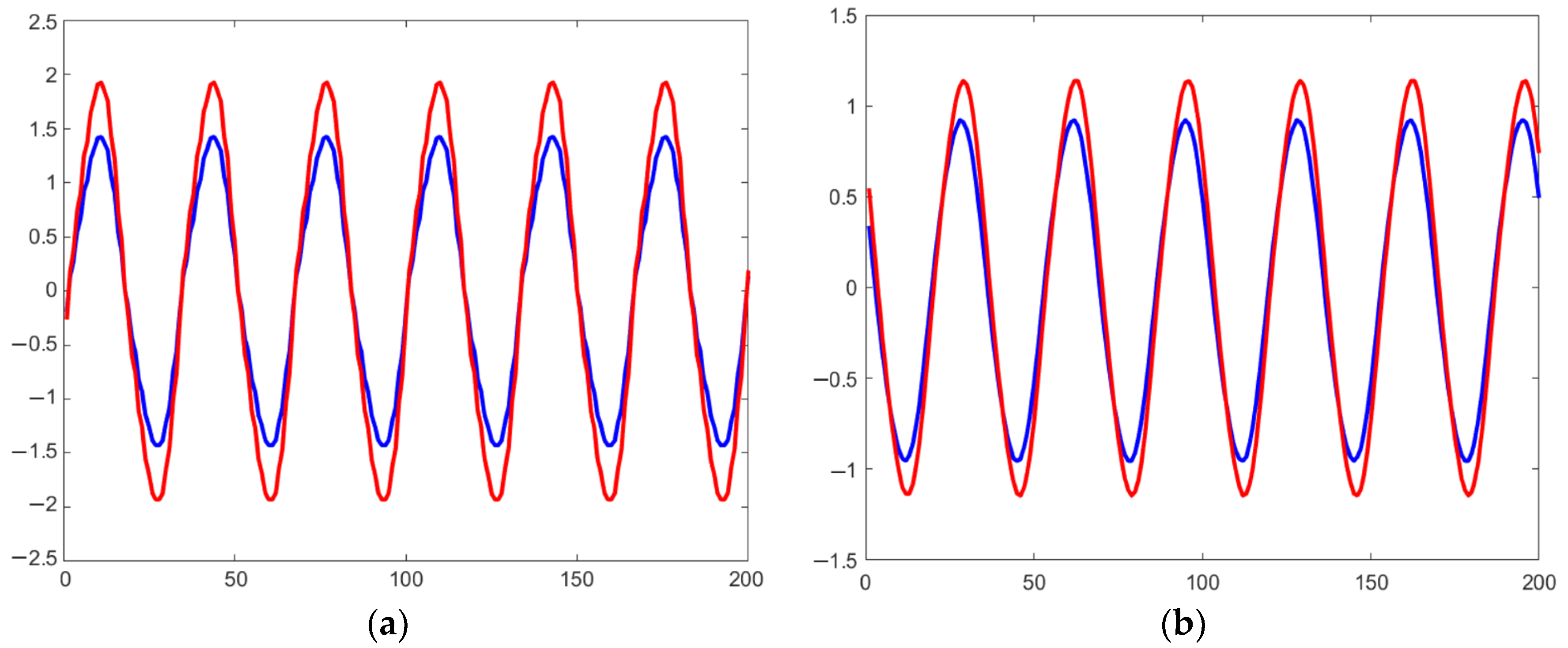
3. Experimental Results

Before any treatment was applied to the samples, two test samples from the same lamination were examined under a microscope at 125×, 250×, 500×, 1250×, and 3750× magnifications, while the other samples were analyzed using the Epstein frame to determine their magnetic properties. After one test sample was heated and rapidly cooled, the samples were prepared with a metallographic grinder, etched, and then analyzed under a microscope, with the laser scan results shown in Figure 6, Figure 7, Figure 8, Figure 9 and Figure 10. Using the laser scan function of the microscope and the software Keyence Vk-X3000 Multifile Analyzer, which allowed us to analyze the profile of the samples, we determined the distance and layer-height difference between different types of grains.

Following the analysis of the profile of the normal sample, we observed that the average distance between grains from the same material was around 1.8 μm, and the average height difference between grains was around 0.002 μm. The average distance between grains of different materials was around 2.2 μm, 22% more than the distance between same-material grains. The height difference was significantly larger, averaging around 0.090 μm.

Based on the analysis of the quenched sample profile, it was observed that the average intergranular distance for grains of the same material was approximately 3.1 μm, with an average height difference of about 0.002 μm. In contrast, the average distance between grains of different materials was approximately 3.6 μm, which was 16% greater than the distance between grains of the same material. The height difference between grains of different materials decreased by 44% compared to the values before quenching, averaging around 0.050 μm. Comparing the results obtained from the scans, we can conclude that the process of quenching increased the intergranular distance of grains by 29% and reduced the height difference between grains by 40%.

After quenching, the samples developed a red hue, which is typically more related to surface phenomena like oxidation; iron oxide (Fe₂O₃), in particular, can impart a reddish color to the steel surface. Residual stresses introduced during quenching can affect the steel’s reflectivity and perceived color under certain lighting conditions. The samples also lost some flexibility and became more rigid, with some samples retaining a warped shape. We analyzed the magnetic proprieties at 0.5 T, 1.0 T, and 1.5 T, at 50 Hz before and after heating. The results are shown in Figure 11 and Figure 12.

At 1.5 T, the coercive force increased by 273% after quenching, indicating a significant loss in the material’s soft magnetic properties. The large coercive field observed in the hysteresis loop, as shown in Figure 11, is characteristic of hard magnetic materials. When compared to the hysteresis at 1 T, the difference in coercive force is even more pronounced, with an increase of 318.5%. At 0.5 T, the coercive force increased by 403.6% after quenching, as depicted in Figure 12.

Before quenching, the hysteresis loop exhibited characteristics typical of soft magnetic materials. At 0.5 T, as shown in Figure 11, the circular shape of the hysteresis loop indicates that the integrated signal used to determine the B field is a cosine wave, implying minimal signal distortion at this value. However, after quenching, the hysteresis loop features a series of “bumps,” which, according to [17] (p. 8), is characteristic of grain-oriented electrical steel at frequencies higher than 50 Hz, specifically at 400 Hz. These “bumps” appear at 1.0 T but are not as pronounced as those seen at 1.5 T. At 0.5 T, the hysteresis loop acquires circular edges, indicating low distortions in the secondary coil voltage.

After analyzing the hysteresis, we sought to understand the effects of quenching on the core of transformers operating at lower current values. We decided to observe the transformer ratio of the Epstein frame at B-field values lower than 0.5 T, as Figure 12 indicates that the secondary sine wave exhibited minimal distortion at these lower values. The primary and secondary voltages were measured at 50 Hz, 100 Hz, and 150 Hz.

In Figure 13a, the voltage measured at the primary coil and the voltage measured at the secondary coil are depicted. The primary coil was connected to a function generator producing a sine wave at 50 Hz, set to 7 V peak-to-peak. Before the thermal treatment of the material, a phase shift of 2 ms was observed. The peak voltage of the primary coil was measured at 1.04 V, and the peak voltage of the secondary coil was 0.62 V, resulting in a transformer ratio of 0.59.

In Figure 13b, the same measurements were performed after quenching. The phase shift between the secondary and primary coils remained at 2 ms. However, the peak voltage of the primary coil decreased to 0.66 V, a reduction of 37.7%, and the peak voltage of the secondary coil decreased to 0.48 V, a reduction of 16.9%. Despite these decreases, the transformer ratio increased to 0.72, which is higher than the ratio before quenching.

In Figure 14a, the voltage measured at the primary coil and the voltage measured at the secondary coil are shown. The primary coil was driven by a function generator producing a sine wave at 100 Hz, set to 7 V peak-to-peak. A phase shift of 2 ms was observed, and the peak voltage of the primary coil was measured at 1.49 V, while the peak voltage of the secondary coil was 1.11 V, resulting in a transformer ratio of 0.74.

In Figure 14b, the same measurements were conducted after quenching. The peak voltage of the primary coil decreased to 0.88 V, and the peak voltage of the secondary coil decreased to 0.72 V. Despite these reductions, the transformer ratio increased to 0.81, which is higher than the ratio observed before quenching.

In Figure 15a, the voltage measured at the primary coil and the secondary coil is illustrated. The primary coil was connected to a function generator generating a sine wave at 150 Hz with a peak-to-peak amplitude of 7 V. A consistent phase shift of 2 ms, as observed in previous measurements, was noted. The peak voltage measured at the primary coil was 1.92 V, and at the secondary coil, it was 1.41 V, resulting in a transformer ratio of 0.72.

In Figure 15b, the same measurements were conducted after quenching. The peak voltage at the primary coil decreased to 1.13 V, and at the secondary coil, it decreased to 0.91 V. Despite these reductions, the transformer ratio increased to 0.80, which is higher than the ratio observed before quenching.

Another parameter analyzed in this study was the specific loss of power, measured across frequencies ranging from 5 Hz to 150 Hz. Quenching the material resulted in a significant increase in the specific loss of power, specifically a 212% increase. Figure 16 illustrates that these losses increased exponentially with frequency, highlighting the critical role of a material’s microstructural integrity.

The observed exponential increase in the power loss with the frequency underscores the importance of microstructural characteristics. For applications in which minimizing AC energy losses is crucial, quenching appears to be an unfavorable option based on these findings.

To test the mechanical properties of the samples, a nano-indenter was used to perform 24 tests on both the pre-quenching and post-quenching samples. The results are presented in Table 1. The intrinsic Young’s modulus of grain-oriented electrical steel (GOES) typically ranges between 100 and 140 GPa, indicating that our sample before quenching fell within the expected parameters for GOES.

According to [18], in the case of high-carbon steel (0.58% C, our sample was at 0.04% C), the intrinsic Young’s modulus decreases with an increase in quenching temperature, being the highest when the sample is quenched at 750 °C. In the case of low-carbon, low-alloy steel (0.08% C) [19], the optimal strengthening and toughness matching can be achieved at 600 °C tempering, the same temperature we used to quench the sample. The increase in Young’s modulus after quenching made the material have lower flexibility and impact toughness and, with the increase in hardness, made the material more brittle. Martensite has, according to [20], a value between 25 and 50 GPa, while ferrite’s value is around 200–230 GPa, cementite’s is in the range of 200–240 GPa, and pearlite’s is 200–220 GPa. Our sample’s mean elasticity modulus of 390 GPa indicates microstructural changes and an increase in the concertation of ferrites, as cementite mostly forms in high-carbon steel (at 0.8% C), and pearlite does not form when quenching. A change in the intrinsic Young’s modulus indicates a great change in the microstructure of the material; while it can be explained by the changes in the distance between the grains, the change seems too little for such a high increase in Young’s modulus. From the results, indicated in

Table 2. Comparison of the Young’s modulus between samples.

Test	Before Quenching		After Quenching
	Apparent Young’s Modulus at Max Load (GPa)	Hardness at Max Load (GPa)	Apparent Young’s Modulus at Max Load (GPa)	Hardness at Max Load (GPa)
1	120.177	1.193	380.93	1.374
2	113.705	1.118	323.635	1.534
3	112.648	1.17	354.86	1.359
4	111.439	1.175	364.595	1.356
5	109.155	1.168	372.029	1.37
6	111.190	1.193	377.441	1.402
7	114.880	1.18	397.917	1.406
8	117.719	1.191	381.132	1.472
9	126.043	1.27	351.378	1.388
10	123.271	1.228	406.845	1.371
11	119.041	1.221	405.842	1.42
12	111.883	1.154	391.293	1.437
13	109.949	1.159	431.857	1.509
14	106.656	1.151	396.091	1.455
15	105.872	1.173	393.955	1.422
16	106.466	1.139	397.064	1.412
17	111.212	1.192	402.179	1.396
18	116.795	1.222	410.156	1.409
19	118.828	1.179	342.078	1.39
20	119.037	1.207	415.618	1.414
21	115.402	1.23	423.066	1.386
22	110.629	1.189	399.734	1.401
23	106.094	1.165	408.321	1.44
24	103.203	1.155	329.408	1.504
Mean	113.387	1.184	394.402	1.419
Std. Dev.	5.877	0.034	27.039	0.047
% COV	5.18	2.83	4.55	3.33

, we can see a 248% increase in the modulus of elasticity and a 19.84% increase in hardness, as shown in the load–displacement curve in Figure 17.

One potential factor contributing to the unusually high Young’s modulus observed during nanoindentation may be the presence of compressive residual stresses. These stresses can cause the material beneath the indenter to resist deformation more than it would in a stress-free condition, thereby increasing the apparent Young’s modulus. The warping observed in the 30-cm samples used in the magnetic test further supports this explanation. The thin geometry of the sample, combined with the high cooling rates associated with water quenching, likely resulted in asymmetric quenching, making uniform cooling unattainable. As a result, the true, intrinsic Young’s modulus of the material is likely closer to the pre-quenching values. To gain a more accurate understanding of the elastic properties, additional testing using nanoindentation techniques, such as the ramp-load pile-up scratch test shown in Figure 18, was required. These tests provided more comprehensive insights into the material’s behavior under such conditions.

To determine the elastic anisotropy of the samples, another series of tests that were performed using nanoindentation were scratch pile-up with ramp-load topographical compensation tests at 0°, 45°, and 90° from the rolling direction, with the maximum load of 20 μN and over a distance of 1 mm, as exemplified in Figure 18. The sample of GO electrical steel has crystal grains aligned in the (110) direction of the body-centered cubic (BCC) lattice, which enhances its magnetic properties in that direction. This grain alignment also leads to strong elastic anisotropy. In GO steel, the rolling direction (RD) has higher stiffness, while the transverse direction (TD) and 45° to the rolling direction exhibit lower stiffness. The results are shown in

Table 3. Elastic anisotropy of the sample.

Status	Degrees	Surface Roughness (Ra)	Elastic Deformation (%)	Plastic Deformation (%)	Pile-Up Height
Before Quenching	0° (RD)	71.6	33.8	66.2	176
	45°	54.1	36.8	63.2	58
	90° (TD)	28.6	37.4	62.6	61
After Quenching	0° (RD)	52.1	39.6	60.4	168
	45°	40.9	42.2	57.8	23
	90° (TD)	23.4	63.2	36.8	29

.

The surface roughness decreased after quenching, as shown in Figure 7 and Figure 9. The reduced pile-up height indicates increased brittleness in the 45° and 90° directions. The increase in elastic deformation and reduction in plastic deformation are characteristics typically exhibited with brittle materials at the beginning of the stress–strain curve.

Having analyzed the data provided by the nanoindenter, including the load–displacement curve, increased hardness, high apparent Young’s modulus, reduced pile-up height, and changes in plastic and elastic deformation, we can conclude that the material became more brittle. One contributing factor was thermal stress. Quenching induces thermal stresses due to the rapid cooling of the outer layers, while the inner core remains hot for a longer period. This differential cooling results in residual stresses within the material, which can lead to cracks or brittle failure. Additionally, quenching may precipitate certain brittle phases, such as carbides, which form between 200 °C and 727 °C along grain boundaries, contributing to grain-boundary embrittlement.

Another factor to consider is hydrogen embrittlement. Quenching in water can introduce hydrogen into steel, which diffuses into the material and increases brittleness. Hydrogen embrittlement often results in delayed failure or cracking after the material has been in service for some time.

Furthermore, silicon embrittlement may be a factor, particularly when the silicon content exceeds 2%. Our sample contained 3.1% silicon. Silicon can impede the movement of dislocations within the steel’s crystal lattice—defects that allow for plastic deformation. When silicon interferes with dislocation movement, steel becomes less ductile and more susceptible to brittle fracture. High silicon content can also lead to the formation of brittle phases or precipitates, such as silicon carbides (SiCs), which often form at grain boundaries or within the matrix, thereby reducing ductility.

4. Discussion

The behavior of electrical steel under heat during normal operations is well documented [8], and the effects of quenching in the manufacturing process of GOES are known, but there is a lack of information regarding the effects of quenching on a finished product and the performance change after such heat treatment since it is not the intended purpose of the material. Furthermore, we consider the results to still be relevant to understanding the material and the effects of quenching on steel alloys below the eutectoid temperature of austenite. After examining various parameters, we can conclude that quenching at 600 °C induces a complex phenomenon, leading to changes in distance and height differences between grains, which are also highlighted by the change in the modulus of elasticity. This surface tends to retain much of its structure post-quenching. In contrast to the structural changes, the magnetic proprieties of the material change significantly. The hysteresis loop prior to quenching exhibits similar characteristics to those studied in [17]; it retains its soft magnetic material properties of a low coercive field. However, post-quenching, the hysteresis loop resembles the shape measured at the 400-Hz-to-1-kHz frequency range, as indicated in [21]. This is significant, as GO electrical steel is optimized for 50-Hz frequencies, suggesting a potential application in situations requiring its magnetic properties at higher frequencies, but it might also indicate a change in the orientation of the magnetic domains of the material.

To comprehend this phenomenon, it is essential to consider the possibility that the substantial change in the magnetic properties of GO electrical steel could be attributed to the presence of “island grains”—contaminants or defects introduced during the manufacturing process [22]. While minor contamination during heating in a furnace or rapid cooling in water may affect magnetic properties marginally, the magnitude of the observed changes suggests otherwise. Moreover, a microscopic analysis of surface contaminants post-quenching was not feasible due to the sample preparation method. Therefore, the marked alteration in magnetic properties is more likely attributable to shifts in grain-structure distances and changes in height differences. A comparable process to quenching is laser cutting, in which heated edges form distinct zones different from the central area and are subsequently rapidly cooled, often with water [23]. Research indicates that, while laser cutting affects the magnetic properties of bundled strips, this influence is relatively minor compared to quenching. In contrast to other low-temperature heat treatments [24,25], which typically preserve the grain shape and structure, quenching significantly modifies inter-grain distances by nearly 30% and reduces height differences by 40%.

Rapid heating is claimed to enhance magnetic properties in soft ferrites [26], non-oriented electrical steel [27], and some magnetic composite materials [28]. Although ultra-rapid heating in the manufacturing process has been proposed to improve the magnetic properties of GO electrical steel [29], quenching or rapid cooling has the opposite effect, deteriorating its magnetic properties. While the Curie temperature is lower than the eutectoid temperature at which austenite forms, the increased nano-indenter hardness presents a primary advantage of quenching.

5. Conclusions

The objective of this research was to examine the alterations induced via quenching on the magnetic properties of grain-oriented (GO) electrical steel, with a focus on changes in material structure changes and mechanical properties (Young’s modulus and hardness).

The key findings include the following:

• Using nanoindentation, we concluded that the brittleness of the material increased; the hardness and apparent Young’s modulus increased following quenching.
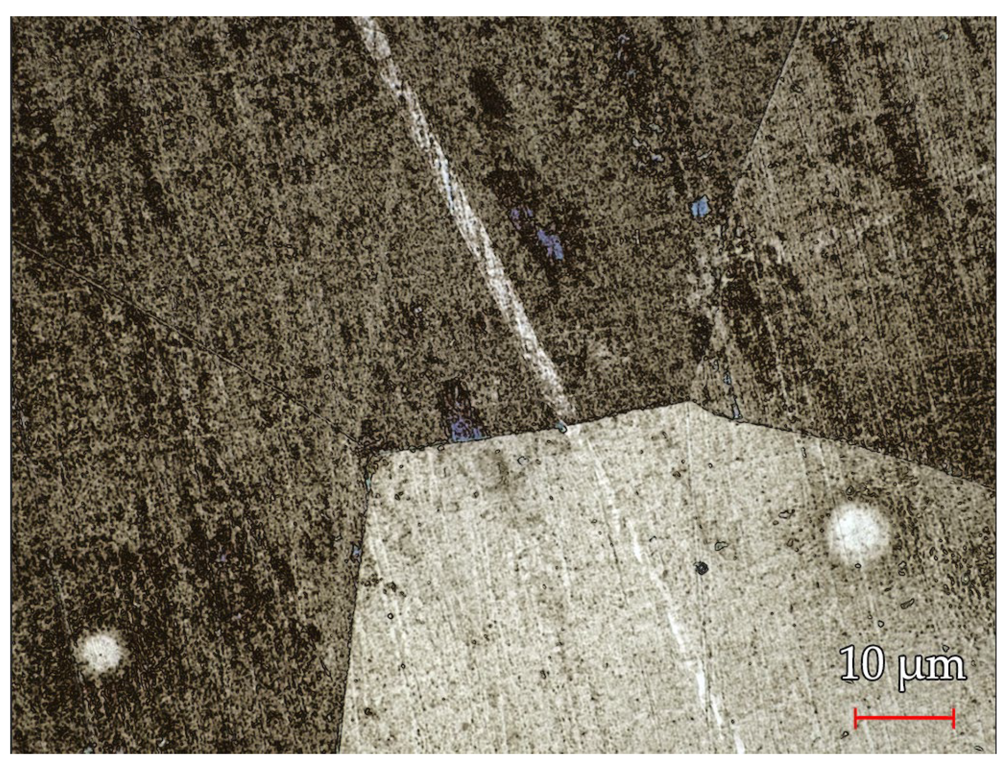
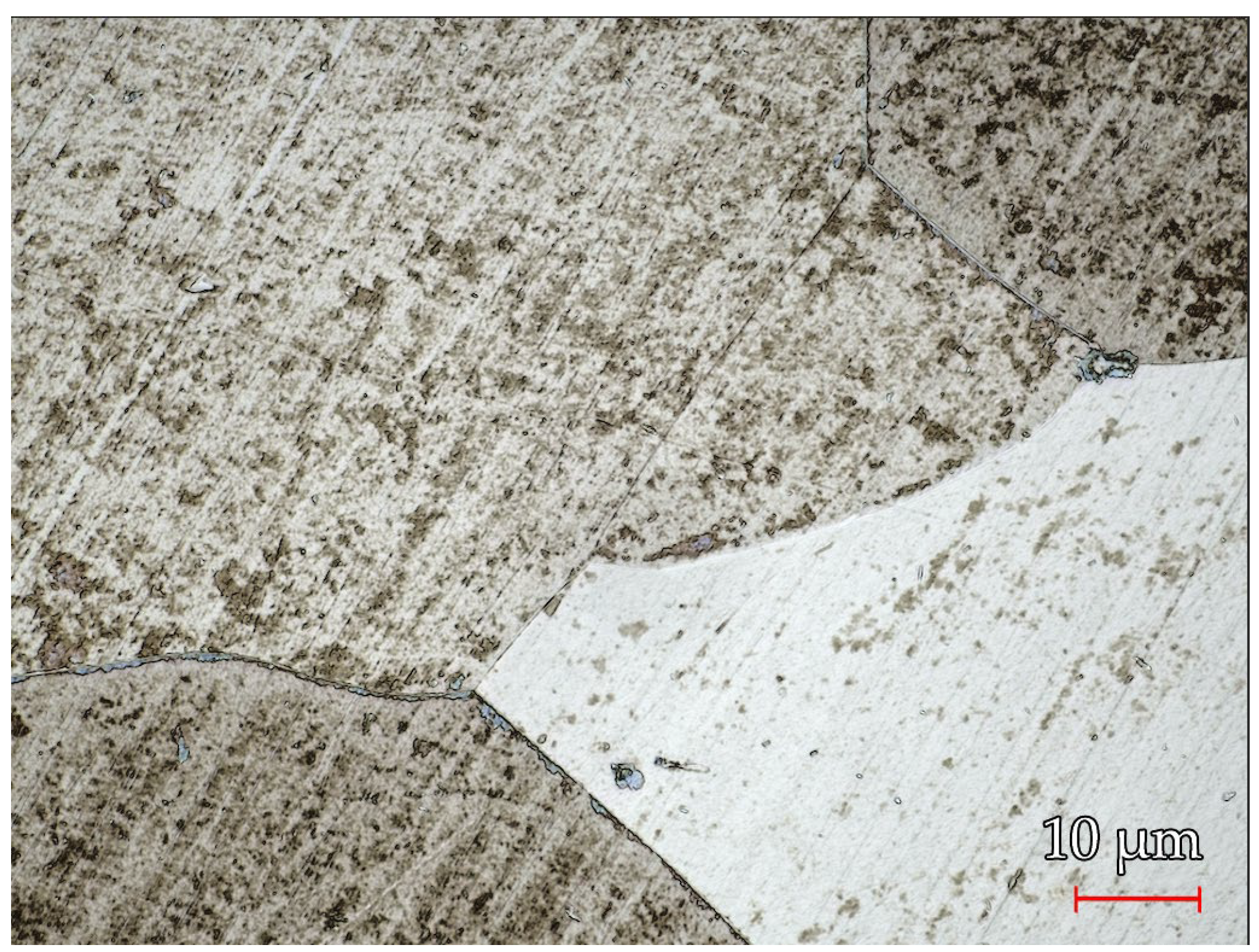
• Using laser microscopy, we concluded that the heat-treatment process affected the distance between grains, increasing it, reducing the height difference between grains, and thus reducing the surface roughness.
• Using the Epstein frame, we concluded that magnetic properties deteriorated post-quenching, evidenced by an increased coercive field, which mirrored the magnetic properties observed at higher frequencies.

The results of this study enhance the understanding of the impact of quenching on GO electrical steel, particularly the phenomenon through which the material exhibits high-frequency magnetic properties at lower frequencies. However, the degraded magnetic properties constrain the applicability of this metallurgical process, rendering it unsuitable for power transformer production. Future research should focus on investigating magnetic properties at lower frequencies, utilizing methods such as those described in [30,31] with the Epstein frame, or the approach in [32], to ensure consistency in results.

References

1. Krings, A.; Boglietti, A.; Cavagnino, A.; Sprague, S. Soft Magnetic Material Status and Trends in Electric Machines. IEEE Trans. Ind. Electron. 2016, 64, 2405–2414. [Google Scholar] [CrossRef]
2. Lopez, S.; Cassoret, B.; Brudny, J.F.; Lefebvre, L.; Vincent, J.N. Grain Oriented Steel Assembly Characterization for the Development of High Efficiency AC Rotating Electrical Machines. IEEE Trans. Magn. 2009, 45, 4161–4164. [Google Scholar] [CrossRef]
3. Xia, Z.; Kang, Y.; Wang, Q. Developments in the production of grain-oriented electrical steel. J. Magn. Magn. Mater. 2008, 320, 3229–3233. [Google Scholar] [CrossRef]
4. Günther, K.; Abbruzzese, G.; Fortunati, S.; Ligi, G. Recent technology developments in the production of Grain-Oriented electrical steel. Steel Res. Int. 2005, 76, 413–421. [Google Scholar] [CrossRef]
5. Elgamli, E.; Anayi, F. Advancements in Electrical Steels: A Comprehensive Review of Microstructure, Loss Analysis, Magnetic Properties, Alloying Elements, and the Influence of Coatings. Appl. Sci. 2023, 13, 10283. [Google Scholar] [CrossRef]
6. Shin, S.; Birosca, S.; Chang, S.; De Cooman, B.C. Texture evolution in grain-oriented electrical steel during hot band annealing and cold rolling. J. Microsc. 2008, 230, 414–423. [Google Scholar] [CrossRef]
7. Krawczyk, J.; Ścibisz, K.; Goły, M.; Śleboda, T. Texture Intensity in Grain-Oriented Steel in the Main Stages of the Production Cycle. Crystals 2024, 14, 107. [Google Scholar] [CrossRef]
8. Bhadeshia, H.K.D.H. 21—Physical Metallurgy of Steels. In Physical Metallurgy, 5th ed.; Laughlin, D.E., Hono, K., Eds.; Elsevier: Amsterdam, The Netherlands, 2014. [Google Scholar]
9. Millan Mirabal, L.A.; Messal, O.; Benabou, A.; Le Menach, Y.; Chevallier, L.; Roger, J.Y.; Ducreux, J.P. Study of the effect of the demagnetizing field in Epstein strips of grain-oriented electrical steels through 3D finite element analysis. COMPEL—Int. J. Comput. Math. Electr. Electron. Eng. 2022, 41, 579–588. [Google Scholar] [CrossRef]
10. Németh, Z.; Kuczmann, M. Measuring and simulating magnetic characteristics using Epstein frame. Pollack Period. 2018, 13, 15–26. [Google Scholar] [CrossRef]
11. Marketos, F.; Zurek, S.; Moses, A. A Method for Defining the Mean Path Length of the Epstein Frame. IEEE Trans. Magn. 2007, 43, 2755–2757. [Google Scholar] [CrossRef]
12. Sievert, J.D. Determination of AC magnetic power loss of electrical steel sheet: Present status and trends. IEEE Trans. Magn. 1984, 20, 1702–1707. [Google Scholar] [CrossRef]
13. Ahlers, H.; Sievert, J.D.; Qu, Q.C. Comparison of a single strip tester and Epstein frame measurements. J. Magn. Magn. Mater. 1982, 26, 176–178. [Google Scholar] [CrossRef]
14. IEC 60404-2; Magnetic Materials—Part 2: Methods of Measurement of the Magnetic Properties of Electrical Steel Sheet and Strips by Means of an Epstein Frame. International Electrotechnical Commission Std: Geneva, Switzerland, 1996.
15. Köçkar, H.; Meydan, T. Specific Power Loss Comparisons of Magnetic Strips Using Standard Epstein Frame. J. Korean Phys. Soc. 2002, 40, 918–920. [Google Scholar]
16. Reimets, N. Revamp of the Epstein Frame Measurement System for Characterizing Magnetic Materials; CERN, TE—Magnets, Superconductors and Cryostats TE-MSC-MM: Geneva, Switzerland, 2018. [Google Scholar]
17. Fiorillo, F. Soft magnetic materials. In Characterization and Measurement of Magnetic Materials, 1st ed.; Mayergoyz, I.D., Ed.; Academic Press: Cambridge, MA, USA, 2004. [Google Scholar]
18. Marthini, V.; Alhelali, I.A.A.; Afendi, M.; Majid, M.; Syafiq, W.M. Effect of Quenching on the Mechanical Properties of Carbon Steel for Hammer Mill. J. Phys. Conf. Ser. 2021, 2051, 012057. [Google Scholar] [CrossRef]
19. Zhang, Y.; Yang, J.; Xiao, D.; Luo, D.; Tuo, C.; Wu, H. Effect of Quenching and Tempering on Mechanical Properties and Impact Fracture Behavior of Low-Carbon Low-Alloy Steel. Metals 2022, 12, 1087. [Google Scholar] [CrossRef]
20. Pham, T.H.; Nguyen, N.V. Mechanical properties of constituent phases in structural steels and heat-affected zones investigated by statistical nanoindentation analysis. Constr. Build. Mater. 2021, 268, 121211. [Google Scholar] [CrossRef]
21. Ducharne, B.; Hamzehbahmani, H.; Gao, Y.; Fagan, P.; Sebald, G. High-Frequency Fractional Predictions and Spatial Distribution of the Magnetic Loss in a Grain-Oriented Magnetic Steel Lamination. Fractal Fract. 2024, 8, 176. [Google Scholar] [CrossRef]
22. Liu, Z.; Yang, P.; Li, X.; Wang, X.; Ma, J.; Liu, G. Formation of island grains in high-permeability grain-oriented silicon steel manufactured by the acquired inhibitor method. J. Phys. Chem. Solids 2020, 136, 109165. [Google Scholar] [CrossRef]
23. Bali, M.; De Gersem, H.; Muetze, A. Epstein frame measurement based determination of original non-degraded and fully degraded magnetic properties of material submitted to mechanical cutting. In Proceedings of the 2015 IEEE International Electric Machines & Drives Conference (IEMDC), Coeur d’Alene, ID, USA, 10–13 May 2015; pp. 1184–1189. [Google Scholar]
24. Stoyka, V.; Kovac, F.; Julius, B. Study of secondary recrystallization in grain-oriented steel treated under dynamical heat treatment conditions. Metalurgija 2009, 48, 99–102. [Google Scholar]
25. Xiao, L.; Yu, G.; Zou, J.; Xu, Y.; Liang, W. Experimental analysis of magnetic properties of electrical steel sheets under temperature and pressure coupling environment. J. Magn. Magn. Mater. 2019, 475, 282–289. [Google Scholar] [CrossRef]
26. Lu, H.; Zhu, J.G.; Hui, S.Y. Measurement and Modeling of Thermal Effects on Magnetic Hysteresis of Soft Ferrites. IEEE Trans. Magn. 2007, 43, 3952–3960. [Google Scholar] [CrossRef]
27. Wang, J.; Li, J.; Wang, X.; Mi, X.; Zhang, S. Rapid heating effects on grain-size, texture and magnetic properties of 3% Si non-oriented electrical steel. Bull. Mater. Sci. 2011, 34, 1477–1482. [Google Scholar] [CrossRef]
28. Ferraris, L.; Franchini, F.; Pošković, E.; Actis Grande, M.; Bidulský, R. Effect of the Temperature on the Magnetic and Energetic Properties of Soft Magnetic Composite Materials. Energies 2021, 14, 4400. [Google Scholar] [CrossRef]
29. Schoen, J.W.; Margerum, D.E. Ultra-Rapid Heat Treatment of Grain Oriented Electrical Steel. European Patent Office EP0334223A3, 1989. [Google Scholar]
30. Pfuetzner, H.; Shilyashki, G.; Palkovits, M.; Galabov, V. Concept for more correct magnetic power loss measurements considering path length dynamics. Int. J. Appl. Electromagn. Mech. 2014, 44, 259–270. [Google Scholar] [CrossRef]
31. Guillaume, P.; Rémi, P.; Lecointe, J.; Brudny, J.F.; Belgrand, T. Three Epstein frames to characterize iron losses and mean path length of grain oriented electrical steel lamination. In Proceedings of the XVII International Symposium on Electromagnetic Fields (ISEF), Valencia, Spain, 10–12 September 2015. [Google Scholar]
32. Xiang, Q.; Cheng, L.; Wu, K. Study on the Single Sheet Measurement Method for AC Magnetic Measurement on Grain-Oriented Electrical Steel. Materials 2023, 16, 1648. [Google Scholar] [CrossRef]
Figure 1. The surface of the GOES sample seen at 125× magnification.
Processes 12 02045 g001
Figure 2. The surface of the GOES sample seen at 250× magnification.
Processes 12 02045 g002
Figure 3. (a) Epstein frame; (b) simulated Epstein frame using FEMM with the corner-joint effect.
Processes 12 02045 g003
Figure 4. Epstein Frame method for measuring magnetic proprieties.
Processes 12 02045 g004
Figure 5. Epstein frame wattmeter method for measuring power loss.
Processes 12 02045 g005
Figure 6. Samples before quenching, taken via a 3D laser scan at 3750×.
Processes 12 02045 g006
Figure 7. Profile analysis (red area) of the height difference between different grains on the sample from Figure 6.
Processes 12 02045 g007
Figure 8. Quenched samples taken via a 3D laser scan at 3750×.
Processes 12 02045 g008
Figure 9. Profile analysis (red area) of the height difference between different grains on the quenched sample from Figure 8.
Processes 12 02045 g009
Figure 10. Before (a) and after (b) quenching, taken via a microscope at 1250× magnification.
Processes 12 02045 g010
Figure 11. (a) Before (red) and after (blue) quenching comparison of the sample BH hysteresis at 1.5 T; (b) before (red) and after (blue) quenching comparison of the sample BH hysteresis at 1 T.
Processes 12 02045 g011
Figure 12. Before (red) and after (blue) quenching comparison of the sample BH hysteresis at 0.5 T.
Processes 12 02045 g012
Figure 13. (a) Secondary (blue) and primary (red) voltage in transformer before quenching at 50 Hz; (b) secondary (blue) and primary (red) voltage in transformer after quenching at 50 Hz.
Processes 12 02045 g013
Figure 14. (a) Secondary (blue) and primary (red) voltage in transformer before quenching at 100 Hz; (b) secondary (blue) and primary (red) voltage in transformer after quenching at 100 Hz.
Processes 12 02045 g014
Figure 15. (a) Secondary (blue) and primary (red) voltage in transformer before quenching at 150 Hz; (b) secondary (blue) and primary (red) voltage in transformer after quenching at 150 Hz.
Processes 12 02045 g015
Figure 16. Specific loss of power before (red) and after (blue) quenching.
Processes 12 02045 g016
Figure 17. The load–displacement curve.
Processes 12 02045 g017
Figure 18. Ramp-load graph and a scratch test at 45° from the rolling direction (RD).
Processes 12 02045 g018