Structural Design Analysis of Substrate with Honeycomb Core Under Normal Pressure, Using RSM and ANN

Abstract

This study presents a comprehensive structural performance analysis of a honeycomb-core substrate under normal pressure, highlighting the superior predictive accuracy of Artificial Neural Networks (ANNs) over Response Surface Methodology (RSM). The analysis focused on critical design parameters, such as material selection, coverage rate, and wall thickness, which significantly influence the substrate’s maximum deformation, elastic stress, and mass. The ANN model, trained on these parameters, optimized the design to achieve a cell size of 60 mm, a wall thickness of 12.5753 mm, a coverage rate of 64.38%, and selected aluminum as the material. This optimization resulted in a substrate with a maximum deformation of 7.21 × 10³ mm, an elastic stress of 1.9465 MPa, and a mass of 54.949 kg. The RSM-ANN method surpasses RSM in both optimization and accuracy, enhancing the understanding of how honeycomb design affects substrate properties.

1. Introduction

With the development of 3D printing technology, Laser Powder Bed Fusion (LPBF) and other additive manufacturing technologies are widely applied [1,2,3]. The performance of printing equipment is pivotal in the printing process, with the load-bearing substrate offering critical support and determining part precision through its resistance to deformation. Excessive deformation can lead to the scrapping of entire batches of parts, resulting in resource loss. The challenge in structural design is ensuring sufficient strength while reducing mass, which has been addressed by researchers through meticulous material selection, geometric design, and manufacturing process optimization.

The design of load-bearing structures is systematically approached to achieve an economical and efficient structural form, optimizing material usage for superior structural performance. The honeycomb structure, revered for its low gravity ratio and high shear modulus, has become a staple in support structure design across automotive, military, and aerospace sectors. This is also the research subject of this study, and the design results can be seen in Figure 1. This systematic and goal-oriented process ensures the minimal material requirement is met to attain the best performance, highlighting the honeycomb structure’s utility in high-stress applications [4,5].

The honeycomb structure is renowned for its ability to minimize substrate mass while maintaining requisite strength, making it a focal point of scientific research due to its exceptional mechanical properties. A variety of honeycomb configurations exist, such as negative Poisson’s ratio honeycombs, hexagonal, circular, square, triangular, and chiral honeycombs, each with unique characteristics, Figure 2. In load-bearing applications, the approach is often targeted towards optimizing cost-effective parameters to achieve the most efficient structural performance with minimal material and cost. Marklolin’s calculations have demonstrated that honeycomb structures are the most material-efficient for a given volume, indicating their optimal topological structure for covering two-dimensional planes. Moreover, honeycomb structures exhibit superior impact resistance compared to single-layer panels, which is a critical consideration in many engineering applications. This enhanced impact resistance is attributed to the structural complexity of honeycombs, which allows for better energy absorption and distribution upon impact. Therefore, the honeycomb structure not only offers a lightweight solution, but also provides significant advantages in terms of mechanical performance and durability [6,7].

Concerns have emerged in the design of honeycomb structures, particularly regarding the constraints of experimental scale, computational complexity, and efficiency. Fortunately, technological advancements have presented potential remedies for these challenges [8,9,10,11,12,13,14,15,16,17,18,19,20,21,22]. To address the escalating demands of experimental research, statistical methodologies have been refined. Descriptive statistics, a prevalent approach, utilize tabulation, classification, and graphical representation to highlight central tendencies within data sets. This method excels at capturing and conveying the essential characteristics of data, offering a holistic view of inherent patterns and distributions. Correlation analysis is pivotal in comparing sample data against hypothesized expected values to ascertain statistical significance, and is primarily utilized for data discrimination rather than specific feature design. In optimizing the instantaneous resistance performance of single-rib reinforced hexagonal honeycombs, the optimal symmetric Latin-hypercube design method was effectively employed [9]. Principal component analysis (PCA) is another statistical technique that simplifies data dimensionality by extracting orthogonal factors, known as principal components, which account for the greatest variance within the data. PCA mitigates computational complexity and storage issues, and tackles multicollinearity among variables, making it ideal for analyzing datasets with interrelated features. Sun has conducted impactful experiments on the response and failure mechanisms of honeycomb panels under impact, and has applied multi-objective optimization to honeycomb panels of varying materials [10]. Response Surface Methodology (RSM) stands out as an efficient and cost-effective approach, providing intuitive visualization of complex relationships, swiftly pinpointing optimal conditions, and offering predictive insights into future scenarios. This methodology enhances computational efficiency in structural design optimization. RSM’s strength lies in its performance analysis capabilities, which form the basis of this study. Despite its advantages, RSM is still subject to experimental scale constraints.

Recent studies have conducted experiments on aluminum honeycombs, as shown in Figure 3, to analyze the force variation during the crushing process under normal pressure. However, these studies have not delved further into the changes in structural properties. Moreover, due to differences in applied forces and model scales, the collapse deformation observed is somewhat different from the deformation caused by normal pressure in honeycomb structures used in industrial production [15].

In solving the problem of experimental scale, many researchers have provided their answers [23,24,25,26,27,28,29,30,31,32,33]. Tran created an ANN model to accurately predict the mechanical properties of the plate based on 1450 analytical-result data points [16]; Gupta studied the nonlinear dynamic behavior of shell panels with a honeycomb structure using the finite element method [17]; Pham utilized the theory of higher-order shear deformation to research the motion characteristics of honeycomb structures under large loads [18]; Zhou focused on studying the deformation behavior and energy absorption characteristics of hollow reentrant honeycomb structures using the finite element method [19]; Sarafrraz’s research indicates that increasing the honeycomb thickness leads to a reduction in the critical buckling load [20]; Anh elucidated the influence of geometry, material parameters, and stiffeners on the vibration of plates under large loads through analytical solutions [21]; Liu used the variational principle to study the composite plates’ static bending [22]; Topa utilized an improved hybrid algorithm, combining particle swarm optimization and genetic algorithms, to optimize the fundamental frequency of the plate [23]; Cho analyzed the large-deflection bending of plates on an elastic foundation according to the von-nonlinear theory [24]; Zhu, based on the first-order shear deformation plate theory, used the finite element method to analyze the bending and free vibration of reinforced plates with different thicknesses [25]; and Huang used the finite element method to analyze the zero-Poisson’s-ratio honeycomb core to enhance the performance of the honeycomb structure [8]. Artificial Neural Networks (ANNs) are distinguished among various methodologies for their proficiency in managing extensive datasets, modeling intricate nonlinear dynamics, automating feature extraction, enabling swift parallel processing, exhibiting fault tolerance, and possessing robust machine learning capabilities. Evidently, ANNs offer greater assistance in addressing challenges typically encountered by statistical methods, compared to alternative approaches.

Similarly, Li used nonlinear finite element methods and ANN to study the ultimate strength of multi-cracked ship panels under axial compression [11]; Tahir applied ANN to predict the buckling load of thin cylindrical shells under axial compression [26]; Pham combined the element method with ANN to study the free vibration response of honeycomb core panels [27]; Wang proposed a boundary strategy based on ANN to strike a balance between accuracy and efficiency [28]; and Mahesh employed the finite element method–ANN approach to study the coupled static parameters of composite laminated plates [29]. In practice, these methods are set as representing optimal prior knowledge, yet they are usually difficult to use for training [30], despite these algorithms having been developed and put into use [12,13,14]. To address the aforementioned issues, researchers have established relevant mathematical expressions for the variation of properties in the honeycomb structure. Mcfarland provided an approximate model for determining the average stress of hexagonal structures [31]; Wierzbicki established a theoretical method based on the principle of minimum plasticity and energy considerations, to obtain the crushing strength of honeycomb core [32]; Liaghat used the minimum plasticity principle and energy considerations theory, taking into account typical folding elements with two angular elements [33]; and Yin obtained the honeycomb‘s average pressure by distinguishing the folding mechanism into two different folding patterns [34]. Many researchers have demonstrated the synergistic benefits of integrating finite element methods with other techniques to enhance data analysis capabilities. Building on this, we opt to merge ANN with RSM to further our investigation.

The majority of studies in performance analysis and structural design have predominantly concentrated on dynamic and bending analyses, neglecting the interplay between deformation, mass, and other critical factors of support structures. This paper is dedicated to exploring the design characteristics of a substrate with a honeycomb structure by integrating RSM and ANN, thereby addressing the aforementioned research gap.

In the quest for lightweight design methodologies for high-strength load-bearing substrates, this study employs finite element analysis to conduct response-surface analysis experiments. Based on these analyses, a radially arranged honeycomb structure was engineered for the substrate, optimizing the structure by reducing material usage while leveraging the honeycomb’s inherent lightweight properties and maintaining strength. To further elucidate the property variations of the honeycomb support structure under diverse parameters, an ANN model was designed and trained, providing a deeper understanding of its behavior.

Currently, there is no research on analyzing the property variation patterns of load-bearing substrates with radial honeycomb support structures under axial compressive stress using response-surface analysis methods combined with ANN methods.

This paper’s main novelties and contributions are as follows:

(1) A predictive ANN model for the design of load-bearing substrate structures was designed;

(2) The correlation model between structural design factors was obtained through RSM, providing the regression model for model training;

(3) The influencing factors of deformation, stress, and mass for the honeycomb structured load-bearing substrate were discussed in detail;

This study investigated the property variations of the honeycomb structure under static compressive loads to explore the trends of deformation, elastic stress, and mass of the load-bearing substrate under different input parameters.

2. Method

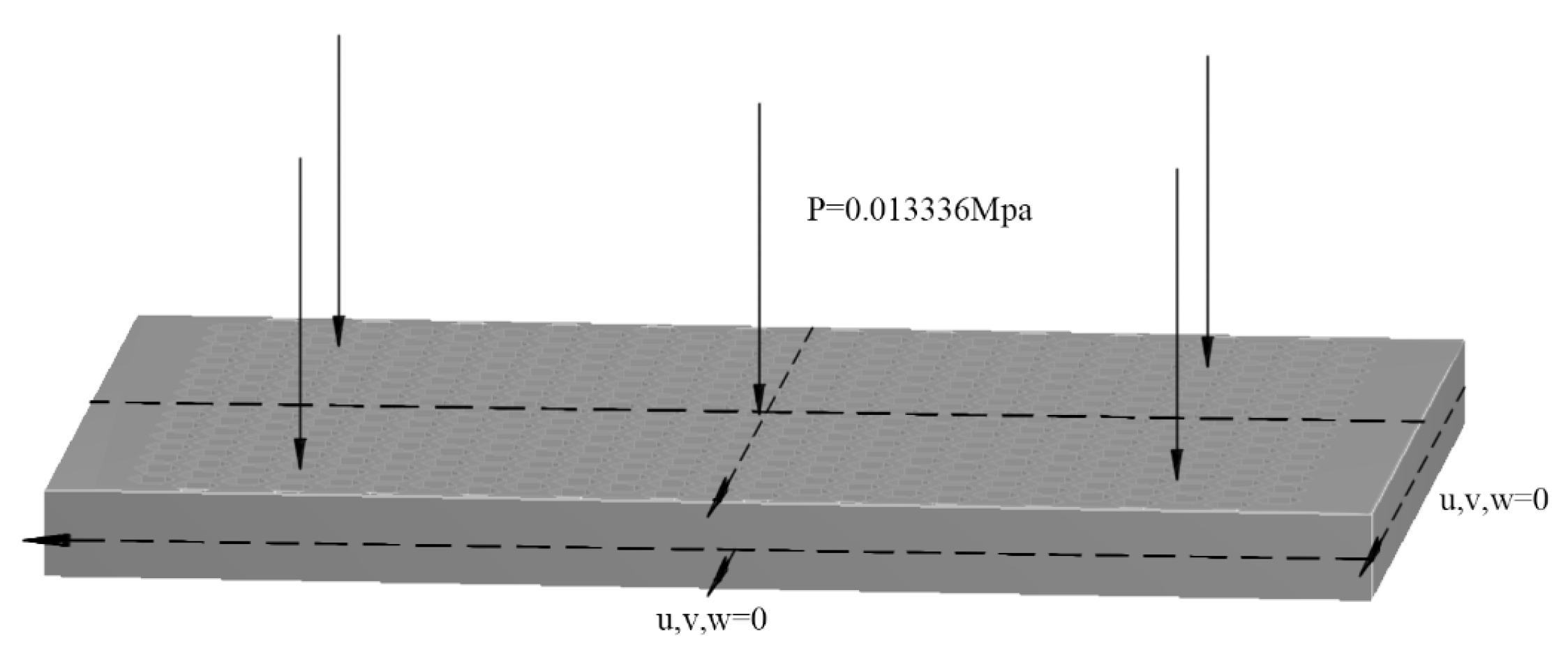
2.1. Problem Description

In this study, a substrate model consisting of honeycomb cells is shown in Figure 4. The geometric dimensions of the plate are length L, width B and thickness H. The Global Cartesian Coordinate System O_xyz is established so that the origin is located at the corner of the middle face of the substrate.

2.2. Finite Elemental Method

Researchers have indeed concentrated on the mathematical formulations of honeycomb structures’ compressive strength, and have established pertinent models. Becker’s analysis has shed light on the impact of node length on honeycomb structure stiffness and the influence of total elastic-core strain energy on crushing distance, providing valuable insights into the mechanics of these structures. This work contributes to the understanding of how structural parameters affect the performance of honeycomb materials under compression [35]. Honeycomb structures consist of vertically arranged rectangular cells, ignoring moments and bending. In-plane stiffness is directly proportional to wall thickness and inversely proportional to cell size [36]; honeycomb cores are predominantly designed to resist shear stress and exhibit enhanced mechanical properties at elevated relative densities. However, the relative density, which is a critical determinant of mechanical performance, is also influenced by the cell size and wall thickness. Smaller cell sizes and thicker walls contribute to the relative density, thereby affecting the structural integrity and performance of honeycomb materials. This interplay between cell geometry and material distribution is crucial for optimizing the mechanical properties of honeycomb structures for various applications.

$${\displaystyle \frac{{\rho }_c}{{\rho }_s}}=({\displaystyle \frac{t}{l}}){\displaystyle \frac{1+\frac{h}{l}}{(\frac{h}{l}+\mathrm{s}\mathrm{i}\mathrm{n}(\theta ))\mathrm{c}\mathrm{o}\mathrm{s}(\theta )}}$$

(1)

where ρ_c is the density of the hexagonal honeycomb core, ρ_s is the density of the base material, t is the thickness of the core, θ is the cell angle, h is the length of the double-cell wall of the hexagonal honeycomb, and l is the length of the single-cell wall of the hexagonal honeycomb.

Sayed argues that the cell wall is fixed at one end and guided at the other end, to determine the modulus [37].

$${\displaystyle \frac{E_1}{E_s}}={({\displaystyle \frac{t}{l}})}^3{\displaystyle \frac{\mathrm{c}\mathrm{o}\mathrm{s}(\theta )}{{\mathrm{s}\mathrm{i}\mathrm{n}}^2(\theta )(\frac{h}{l}+l\mathrm{s}\mathrm{i}\mathrm{n} (\theta ))}}$$

(2)

$${\displaystyle \frac{E_2}{E_s}}={({\displaystyle \frac{t}{l}})}^3{\displaystyle \frac{(\frac{h}{l}+l\mathrm{s}\mathrm{i}\mathrm{n} (\theta ))}{{\mathrm{c}\mathrm{o}\mathrm{s}}^3(\theta )}}$$

(3)

$${\displaystyle \frac{G_{12}}{E_s}}={({\displaystyle \frac{t}{l}})}^3{\displaystyle \frac{(\frac{h}{l}+l\mathrm{s}\mathrm{i}\mathrm{n} (\theta ))}{{(\frac{h}{l})}^2(1+2\frac{h}{l})\mathrm{c}\mathrm{o}\mathrm{s} (\theta )}}$$

(4)

$$v_{12}={\displaystyle \frac{{\mathrm{c}\mathrm{o}\mathrm{s}}^2(\theta )}{\mathrm{s}\mathrm{i}\mathrm{n} (\theta )(\frac{h}{l}+l\mathrm{s}\mathrm{i}\mathrm{n} (\theta ))}}$$

(5)

where E_s is the modulus of elasticity of the base material, E₁ is the modulus of elasticity of the honeycomb in the x-direction, G₁₂ is the shear modulus of the honeycomb in the x-y plane, and v₁₂ is the Poisson’s rate.

Li’s research employed the homogenization technique to scrutinize the influence of honeycomb thickness on mechanical properties and elastic modulus. Finite element simulation methods were utilized to derive effective stress–strain curves, local stress values, and deformation amounts, providing a comprehensive analysis of the structural integrity [38]. Sorohan replaced the honeycomb structure with a homogeneous orthotropic solid structure, and used the model to obtain mechanical properties [39]; the numerical approximations of the homogenized orthotropic solid structure closely align with the outcomes of the original numerical analyses. Salehi has adeptly employed a three-dimensional elastic graded finite-element method, accounting for the continuity of plate thickness, stretching, and material properties. This approach circumvents the limitations inherent in approximate plate theories and conventional finite element methods, yielding more precise analytical results for the shear buckling of functionally graded-material annular-sector plates [40]. Therefore, this paper adopts the homogenized model to simulate the behavior of the honeycomb structure.

Under compressive loading, honeycomb structures are regarded as regular and symmetrical cylindrical columns, where the compression behavior of each cell is a function of its shape and geometric constraints. This perspective is crucial for understanding the mechanical response of honeycombs to compression [16]. The definition of average stress is as follows:

$${\sigma }_m={\sigma }_y{({\displaystyle \frac{t}{S}})}^2[{\displaystyle \frac{4.75}{K}}+28.628]+1.155q_y{\displaystyle \frac{t}{s}}$$

(6)

where σ_m is the mean crushing stress of the honeycomb, σ_y is the yield stress of the honeycomb material, S is the cell minor diameter, K is the width of the basic element size, and q_y is the shear yield stress of the material.

Based on the homogenized honeycomb structure (see Figure 5), a response-surface experiment was designed with substrate material, honeycomb-cell shape, honeycomb-cell-wall thickness, cell size, and coverage rate as experimental factors, and the maximum deformation of the support substrate, mass, and equivalent elastic stress as response factors.

The goal was to analyze factors affecting the support substrate’s maximum deformation, mass, and elastic stress, and to develop a regression model for predicting these under varying conditions. In this study, θ = 120°, t = 50 mm, h = 2 L, and t, s, k, ρ are correlated with the experimental factors, and the finite element model can be seen in Figure 6. Taking into account the aforementioned models for calculation, combined with industrial design requirements and actual working conditions (that is, the substrate load T is approximately 1.4 t/m³ for a fixed-size printing area, and the maximum deformation of the plate within the printing-layer-thickness range of 0.2 mm to 0.5 mm should not exceed 0.01 mm, while considering computational resources and work efficiency), the appropriate value range for each experimental factor required for the RSM is calculated.

2.3. Mesh Convergence Study

The mesh convergence process was systematically executed, commencing with a coarse mesh to ascertain the model’s basic behavior. This initial computational analysis provided a baseline for model response. Subsequent refinements incrementally increased element density, thereby improving model resolution. Each refinement was accompanied by a re-analysis, with outcomes meticulously compared to prior results to ensure convergence accuracy. This cycle of refinement and analysis persisted until the solution reached a state of convergence, indicating that further increases in mesh density would not yield significant changes in the analysis outcomes. The min size limit of the element is 8 mm, the minimum edge length is 15.808, the average element quality is 0.76531, and the average warping factor is 4.891 × 10⁻¹⁵, satisfying the experimental needs.

2.4. Response-Surface Method

Taking wall thickness (a), size (b), coverage rate (c), material (d), and shape (e) as experimental factors, among them, two levels are designed for material and shape, and three levels are designed for wall thickness, size, and coverage rate. The experiment was conducted with maximum deformation (Y₁), elastic stress (Y₂) and mass (Y₃) as response factors; experimental factors and levels can be seen in

Table 1. Experimental factor-level table.

Level	A Size/mm	B Wall Thickness/mm	C Coverage/%	D Material	E Shape
−1	30	5	100	steel	hexagonal
0	60	10	66.5
1	90	15	33	aluminum	circular

, and the schematic of the experimental factors is shown in Figure 7.

2.5. Artificial Neural Network Method

The experimental scope is constrained by the number of trials, rendering the derived regression model suitable primarily for design reference, rather than for precise predictions across varying design factors. To overcome this issue, an ANN model was established, see Figure 8. ANN is an algorithmic model that simulates the structure of neural networks in the human brain. It consists of multiple neurons, which are divided into three layers: the input layer, the hidden layers, and the output layer. Utilizing outcomes from RSM, we optimize the number of hidden layers and neurons within these layers, to enhance the model’s predictive accuracy. Detailed codes have been submitted which can be seen in Appendix A.1, Appendix A.2 and Appendix A.3.

By analyzing the mathematical model of the honeycomb, we selected the influencing factors and determined their value ranges. Furthermore, experiments were conducted to obtain the regression model for the response objectives. On this basis, a dataset is constructed by generating 2000 random and uniformly distributed data vectors through code, with 80% used for training purposes and the remaining 20% for testing, which can also solve the sample imbalance problem. Next, an ANN model with 7 hidden layers was designed to predict the maximum deformation, maximum elastic stress, and mass of the plate under pressure. To evaluate the accuracy and performance of the artificial neural network model, the mean square error (MSE) was used as the evaluation metric. The MSE is defined as follows:

$$\mathrm{MSE}={\displaystyle \frac{1}{n}}\sum _{i=1}^n(Y_i-{\hat{Y}}_i{)}^2$$

(7)

where Y_i − ${\hat{Y}}_{\mathrm{i}}$ is the true value and the predicted value.

3. Results and Discussions

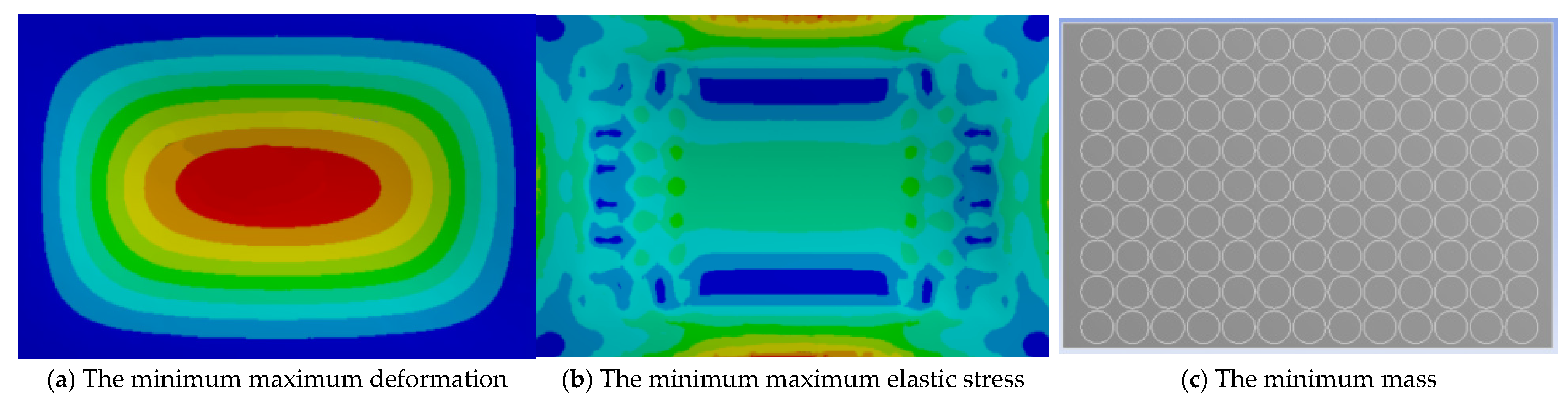
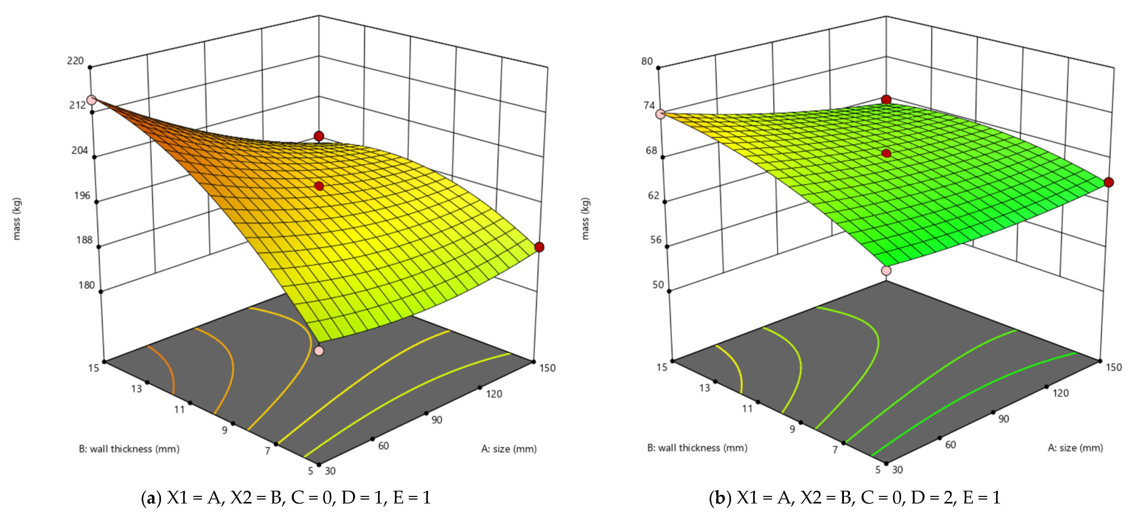
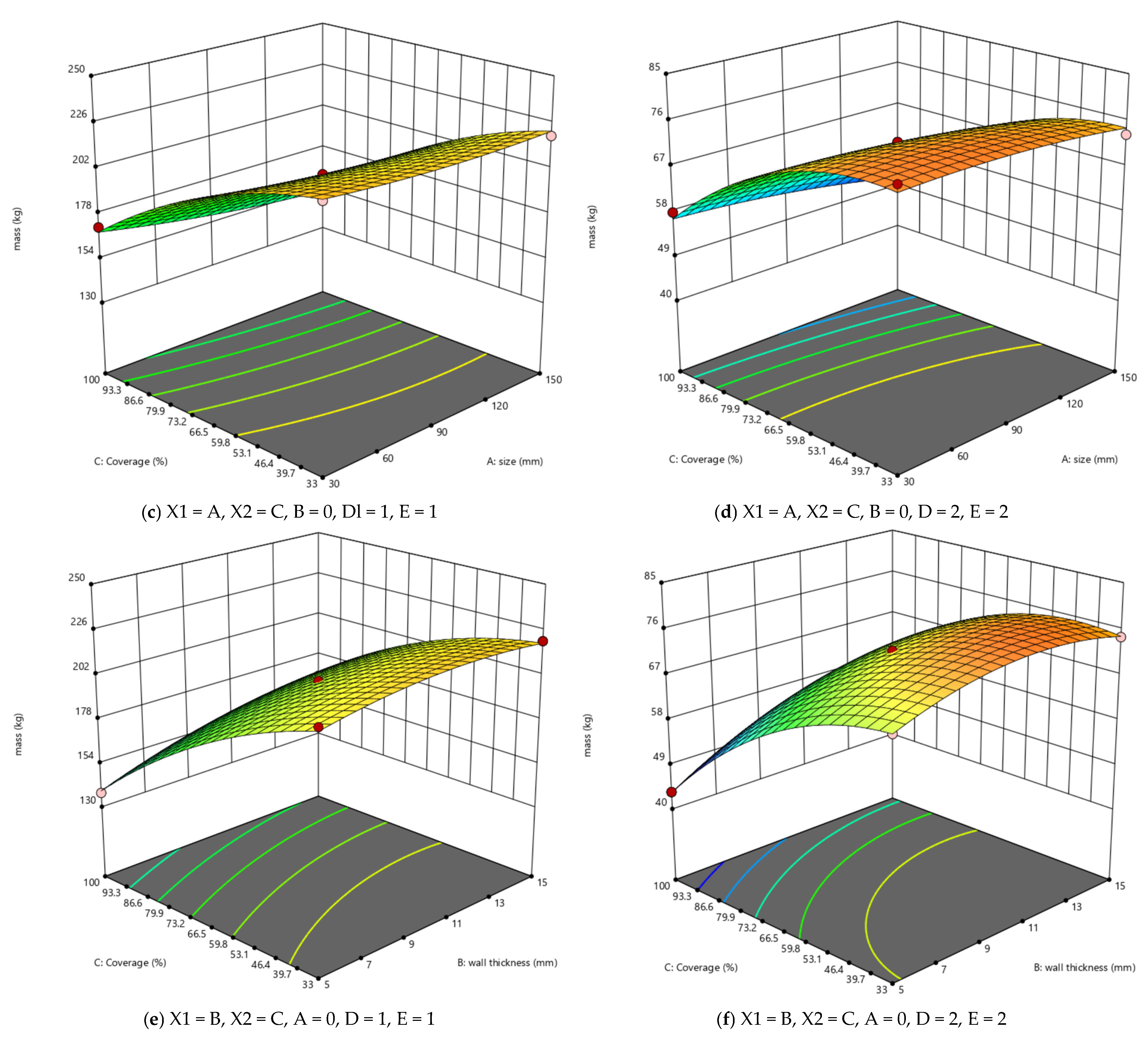
3.1. RSM Results Analysis

The experimental data can be seen in Figure 9, and detailed experimental plans and results can be seen in Appendix A.4.

Settings. Bounding conditions and geometry can be seen in Figure 10. The surroundings are fixed, and the loading type is the pressure, which is p = 0.013336 Mpa. The other parameters can be seen in Table 1 and Figure 7.

Feature Data Analysis. From Figure 11, the analysis indicates that the deformation at the plate’s center forms an elliptical pattern along the longer edge, suggesting that a more uniform stress distribution can mitigate maximum deformation. The maximum elastic stress is localized at the corners of the longer edge, with a low-stress rectangular annular zone observed. Circular structures exhibit lower utilization and resistance to deformation compared to hexagonal ones, and increasing the coverage rate significantly reduces mass without substantially affecting deformation.

Sobol Sensitivity Analysis. The goal is to evaluate the maximum deformation, elastic stress, and sensitivity of quality in designing parameters under normal pressure, and quantifying the impact of input variables on model output variability based on data from Section 3.1.

The definition of the first-order Sobol index and total-effect Sobol index are as follows:

$$S_i={\displaystyle \frac{Var\left(E\right[Y\mid X_i\left]\right)}{Var\left(Y\right)}}$$

(8)

$$T_i={\displaystyle \frac{Var\left(E\right[Y\mid X_1,X_2,\dots ,X_i\left]\right)}{Var\left(Y\right)}}$$

(9)

where S_i is the first-order Sobol index, and T_i is the total-effect Sobol index.

The results of the calculation are as follows:

S_thickness = 0.35, S_size = 0.25, S_coverage = 0.15, S_material = 0.12, S_shape = 0.03;

T_thickness = 0.45, T_size = 0.35, T_coverage = 0.25, T_material = 0.18, T_shape = 0.05.

Thickness and size are the most sensitive model parameters, significantly affecting output. The shape and material’s first-order and total-effect indices are low, suggesting minor individual impacts and weak interactions with other parameters. Detailed analysis will be conducted in Section 3.1.

Maximum Deformation Analysis. We performed a multiple regression analysis on the five factors, to obtain the coded regression equation; the results of the ANOVA can be seen in

Table 2. Response 1: Maximum deformation.

Source	Sum of Squares	df	Mean Square	F-Value	p-Value
Model	0.000263178	18	1.46 × 10−5	23.1	<0.0001	significant
A—size	2.77 × 10−6	1	2.77 × 10−6	4.38	0.0441	**
B—wall thickness	1.00 × 10−5	1	1.00 × 10−5	15.8	0.0004	**
C—Coverage	1.58 × 10−5	1	1.58 × 10−5	24.97	<0.0001	**
D—material	0.000177342	1	0.000177342	280.17	<0.0001	**
E—shape	1.42 × 10−6	1	1.42 × 10−6	2.24	0.1438
AB	4.95 × 10−8	1	4.95 × 10−8	0.0782	0.7815
AC	5.64 × 10−8	1	5.64 × 10−8	0.0891	0.7672
AD	5.57 × 10−7	1	5.57 × 10−7	0.8792	0.3552
AE	1.54 × 10−7	1	1.54 × 10−7	0.2433	0.6251
BC	3.15 × 10−6	1	3.15 × 10−6	4.98	0.0326	**
BD	2.44 × 10−6	1	2.44 × 10−6	3.85	0.0582	*
BE	1.31 × 10−6	1	1.31 × 10−6	2.07	0.16
CD	3.45 × 10−6	1	3.45 × 10−6	5.45	0.0258	**
CE	7.51 × 10−8	1	7.51 × 10−8	0.1186	0.7327
DE	4.27 × 10−7	1	4.27 × 10−7	0.674	0.4176
A2	2.94 × 10−7	1	2.94 × 10−7	0.4648	0.5002
B2	1.34 × 10−6	1	1.34 × 10−6	2.11	0.1555
C2	3.29 × 10−5	1	3.29 × 10−5	52.01	<0.0001	**
Residual	2.09 × 10−5	33	6.33 × 10−7
Cor Total	0.0002	51

* indicates a significant effect of the test factor, ** indicates a highly significant effect of the test factor.

. From the results, it is shown that in the model, p < 0.0001, R² = 0.9265; the multiple regression equation shows a highly significant model with a good fit, effectively reflecting the relationship between factors and the comprehensive score. The factor influence order is material > coverage rate > wall thickness > size > shape, with factors a, b, c, and d having a highly significant impact.

In the response surface graph, the steeper the graph, the greater the influence of the factor on the result. In Figure 12, it is observed that with constant material and shape, deformation increases uniformly as wall thickness decreases and size increases, peaking when both are at their maximum values. The change is stable, without significant fluctuations, and the interaction effect is linear, indicating interaction. With constant wall thickness and material, deformation first decreases then increases with coverage rate, reaching a minimum at 66.7% coverage. As size increases, deformation peaks at 90 mm, with a relatively flat curve compared to coverage rate changes. Interactions increase the deformation’s curve-fitting rate with influencing factors. With aluminum alloy, interactions are more pronounced. With constant size and material, wall thickness and coverage rate significantly interact; deformation decreases with thicker walls and shows a trough at 15 mm wall thickness and 59.8% coverage rate. The maximum deformation regression equation is as follows:

Y1 = 0.0025 + 0.0003A − 0.0006B + 0.0007C + 0.0018D − 0.0004BC − 0.0003BD + 0.0003CD + 0.0019C²

(10)

Maximum Elastic-Stress Analysis. The results of the ANOVA can be seen in

Table 3. Response 2: Maximum elastic stress.

Source	Sum of Squares	df	Mean Square	F-Value	p-Value
Model	16.5389	18	0.9188	14.6809	0.0000	significant
A—size	0.0016	1	0.0016	0.0256	0.8739
B—wall thickness	4.8678	1	4.8678	77.7768	0.0000	**
C—Coverage	1.6893	1	1.6893	26.9916	0.0000	**
D—material	0.0230	1	0.0230	0.3679	0.5483
E—shape	0.9959	1	0.9959	15.9117	0.0003	**
AB	0.0022	1	0.0022	0.0350	0.8527
AC	0.0043	1	0.0043	0.0690	0.7944
AD	0.0118	1	0.0118	0.1881	0.6673
AE	0.0968	1	0.0968	1.5459	0.2225
BC	0.6424	1	0.6424	10.2645	0.0030	**
BD	0.0003	1	0.0003	0.0049	0.9444
BE	1.7888	1	1.7888	28.5810	0.0000	**
CD	0.0185	1	0.0185	0.2948	0.5908
CE	0.1283	1	0.1283	2.0497	0.1616
DE	0.0092	1	0.0092	0.1467	0.7042
A2	0.0230	1	0.0230	0.3673	0.5486
B2	0.8124	1	0.8124	12.9801	0.0010	**
C2	4.7081	1	4.7081	75.2260	0.0000	**
Residual	18.608	51
Cor Total	0.00165	1	0.0016	0.0255	0.8739

** indicates a highly significant effect of the test factor.

. From the results, it is shown that in the model, p < 0.0001, R² = 0.889; the multiple regression equation is highly significant, indicating a good model fit that effectively captures the relationship between factors and the overall score. The factor impact order is wall thickness > coverage rate > shape > material > size, with wall thickness, coverage rate, and shape having the most significant impact.

From Figure 13, the findings reveal that the shape factor substantially influences the interaction between wall thickness and coverage rate, given constant size and material conditions. The hexagonal configuration demonstrates a more pronounced interactive effect compared to the circular one, resulting in a more stable response plot. Higher deformation and steeper edge slopes are observed under the circular unit structure, underscoring the stability benefits of the hexagonal structure. Deformation initially decreases and then increases with the coverage rate, while it exhibits a decreasing trend with wall thickness.

In practice, a larger wall thickness and 60% coverage rate are more likely to achieve ideal deformation, but result in greater mass. Balancing these factors will be discussed in the subsequent sections. The maximum elastic-stress equation is as follows:

Y2 = 0.6896 − 0.39B + 0.2298C + 0.1384E − 0.2004BC − 0.2364BE + 0.2981B² + 0.7176C²

(11)

Mass Analysis. The results of the ANOVA can be seen in

Table 4. Response 3: mass.

Source	Sum of Squares	df	Mean Square	F-Value	p-Value
Model	223,986.04	39	5743.2319	394.0750	0.0000	significant
A—size	384.1923	1	384.1923	26.3616	0.0002	**
B—wall thickness	1854.9075	1	1854.9075	127.2755	0.0000	**
C—Coverage	14,322.27	1	14,322.2735	982.7307	0.0000	**
D—material	17,800.89	1	17,800.8964	1221.4183	0.0000	**
E—shape	36.5541	1	36.5541	2.5082	0.1392
AB	84.4239	1	84.4239	5.7928	0.0331	*
AC	67.1252	1	67.1252	4.6058	0.0530	*
AD	90.9934	1	90.9934	6.2436	0.0280	*
AE	1.6124	1	1.6124	0.1106	0.7452
BC	341.4734	1	341.4734	23.4304	0.0004	**
BD	439.4649	1	439.4649	30.1541	0.0001	**
BE	97.9125	1	97.9125	6.7183	0.0236	**
CD	3393.0674	1	3393.0674	232.8172	0.0000	**
CE	0.0056	1	0.0056	0.0004	0.9847
DE	8.6671	1	8.6671	0.5947	0.4555
A2	0.7234	1	0.7234	0.0496	0.8274
B2	273.7032	1	273.7032	18.7803	0.0010	**
C2	781.1391	1	781.1391	53.5983	0.0000	**
BCD	80.9280	1	80.9280	5.5529	0.0363	*
B2D	64.8357	1	64.8357	4.4487	0.0566	*
C2D	185.0323	1	185.0323	12.6961	0.0039	**
C2E	73.7215	1	73.7215	5.0584	0.0441	*
Residual	174.8874	12	14.5739
Cor Total	224,160.93	51

* indicates a significant effect of the test factor, ** indicates a highly significant effect of the test factor.

. From the results, it is shown that in the model, p < 0.0001, R² = 0.9992; the multiple regression equation is highly significant, indicating a well-fitting model that effectively captures the relationship between factors and the comprehensive score. The influence of factors on the response objective is ranked as wall thickness > coverage rate > material > size > shape, with factors a, b, c, and d being highly significant.

From Figure 14, the influence of material on maximum deformation is significantly more pronounced with steel compared to aluminum alloy, with disparities intensifying as various influencing factors are altered. When steel is utilized, mass is affected more markedly than with aluminum alloy, indicating that higher material density and strength necessitate stricter experimental parameter ranges in the structural-optimization design process.

At a constant coverage rate and material, mass diminishes with decreasing wall thickness and increasing size, exhibiting a gentle, linear relationship with a lower slope. With wall thickness and material held constant, mass markedly decreases as coverage rate increases. Variations in size, influenced by changes in coverage rate, result in more substantial mass reduction at higher coverage rates, albeit to a limited extent. When size and material are constant, reducing the coverage rate and increasing wall thickness lead to a mass increase, with interactive effects analogous to those observed when wall thickness and material are held constant. Although the interactive effects among factors are less pronounced in mass compared to deformation and elastic stress, the linear variations of certain influencing factors significantly affect mass. The mass equation is as follows:

Y3 = 37.06 − 3.46A + 7.61B − 21.16C − 66.71D − 2.3AB − 2.05AC + 1.69AD + 4.62BC − 3.71BD + 1.75BE + 10.3CD − 5.47B² − 9.24C² − 2.25BCD + 2.66B²D + 4.5C²D − 2.84C²E

(12)

3.2. ANN Results

Model Performance Evaluation. In Figure 15, a comparison reveals the alignment between predicted and calculated values, alongside error metrics and the convergence of the MSE loss function. The majority of predictions fall within a narrow margin, with a minority exhibiting larger discrepancies, potentially attributable to the limited depth and iteration count of the network. Nonetheless, even for these outliers, predictions remain within an acceptable range. The congruence between the outcomes of the two distinct methods is evident. The loss functions decrease with each iteration, eventually attaining a stable, convergent value. The MSE values for Y₁, Y₂, and Y₃ are 1.671 × 10⁻⁵, 2.629 × 10⁻⁵, and 2.063 × 10⁻⁶, respectively. Therefore, it can be concluded that the ANN model is suitable for predicting the maximum deformation, maximum elastic stress, and mass properties of the plate under different design parameters.

RSM vs. RSM-ANN. The results of the response optimization design targeting Min Y₁, Min Y₂, and Min Y₃ are

A = 30.0005 mm, B = 12.5753 mm, C = 64.38%, D = Aluminum, E = Hexagonal. Based on the comprehensive evaluation system for the compressive performance of the plate material, we have designed similar evaluation indicators.

$$Z={[1-{\displaystyle \frac{y_1}{y_{1\max }}}]}^{\alpha }+{[1-{\displaystyle \frac{y_2}{y_{2\max }}}]}^{\beta }+{[1-{\displaystyle \frac{y_3}{y_{3\max }}}]}^{\gamma }$$

(13)

From 8000 sets of predicted data (generated by the ANN model), the highest score obtained is 0.969, and the corresponding results are as follows:

In Figure 16, it can be seen that the optimization design results adopted were AL and hexagonal, both in RSM and RSM-ANN, which is consistent with the trend in the previous analysis results.

In the RSM group, Y₁ = 4.81 × 10⁻³ mm, Y₂ = 1.5019 Mpa, and Y₃ = 73.312 kg; in the RSM-ANN group, Y₁ = 7.21 × 10⁻³ mm, Y₂ = 1.9465 Mpa, and Y₃ = 54.949 kg; the RSM-optimized design outperforms the RSM-ANN method in terms of maximum deformation and stress. This superiority stems from the RSM group’s lower coverage rate, resulting in a heavier mass compared to the RSM-ANN plate. Nonetheless, both designs satisfy industrial production standards, with a maximum deformation limit of 0.01 mm and adequate strength. The RSM-ANN plate’s lighter weight suggests more efficient material usage and enhanced feasibility for processing, repair, and installation.

3.3. Discussions

The force distribution within the RSM-ANN group’s plate is characterized by a rectangular pattern, with the low-stress rectangular annular zone being closer to the plate’s edge, which is distinctly superior to the elliptical stress distribution observed in the RSM group. This superiority is attributed to the larger size and relatively thinner walls of the RSM-ANN group, leading to a higher density of honeycomb units and a more uniform stress distribution, thereby enhancing structural utilization efficiency.

4. Conclusions

Given the applications with honeycomb, studying the impact of their design parameters is crucial for the optimized design of such structures. By comparing these with existing numerical results, the accuracy of the method and the results has been verified. Here are conclusions drawn from this paper:

The axially distributed honeycomb structure enhances substrate efficiency, ensuring equivalent load capacity at lower mass.

Influence order on deformation: Material > Coverage > Thickness > Size > Shape; on stress: Thickness > Coverage > Shape > Material > Size; on mass: Thickness > Coverage > Material > Size > Shape. The properties of the load-bearing substrate are optimized at a cell size of 60 mm, with hexagonal structures demonstrating superior performance over circular ones. An increase in wall thickness significantly affects stress distribution, but also contributes to greater mass. The choice of material profoundly influences property variations, in line with the material’s inherent property trends. This study illustrates the enhanced performance of the proposed RSM-ANN methodology compared to RSM alone by evaluating the performance across different experimental groups. Future work will delve into a broader spectrum of parameters to further refine the understanding of structural behavior.

5. Limitations

The response-surface experiments are limited in scale, and may not cover all design parameter combinations, impacting the model’s generalizability. The neural network model, though accurate, relies heavily on the quality and quantity of training data, and lacks interpretability. Computational constraints and differences between experimental and real-world loading conditions are also noted. Environmental factors like temperature and humidity, which can significantly influence material performance, are not considered.

Future research should explore a wider range of structural parameters, material properties, and loading conditions to enhance the model’s predictive capabilities. In summary, while this study provides a valuable method for structural performance prediction, it must be applied with an understanding of its limitations and further validated in future studies.

References

1. Espalin, D.; Muse, D.W.; MacDonald, E.; Wicker, R.B. 3d printing multifunctionality: Structures with electronics. Int. J. Adv. Manuf. Technol. 2014, 72, 963–978. [Google Scholar] [CrossRef]
2. Ngo, T.D.; Kashani, A.; Imbalzano, G.; Nguyen, K.T.; Hui, D. Additive manufacturing (3d printing): A review of materials, methods, applications and challenges. Compos. Part B Eng. 2018, 143, 172–196. [Google Scholar] [CrossRef]
3. Wen, S.; Shen, Q.; Wei, Q.; Yan, C.; Zhu, W.; Shi, Y.; Yang, J.; Shi, Y. Material optimization and post-processing of sand moulds manufactured by the selective laser sintering of binder-coated al2o3 sands. J. Mater. Process. Technol. 2015, 225, 93–102. [Google Scholar] [CrossRef]
4. Shirzad, M.; Zolfagharian, A.; Bodaghi, M.; Nam, S.Y. Auxetic metamaterials for bone-implanted medical devices: Recent advances and new perspectives. Eur. J. Mech.-A/Solids 2023, 98, 104905. [Google Scholar] [CrossRef]
5. Jiang, W.; Ren, X.; Wang, S.L.; Zhang, X.G.; Zhang, X.Y.; Luo, C.; Xie, Y.M.; Scarpa, F.; Alderson, A.; Evans, K.E. Manufacturing, characteristics and applications of auxetic foams: A state-of-the-art review. Compos. Part B Eng. 2022, 235, 109733. [Google Scholar] [CrossRef]
6. Sadikbasha, S.; Pandurangan, V. High velocity impact response of sandwich structures with auxetic tetrachiral cores: Analytical model, finite element simulations and experiments. Compos. Struct. 2023, 317, 117064. [Google Scholar] [CrossRef]
7. Novak, N.; Al-Rifaie, H.; Airoldi, A.; Krstulovi´c-Opara, L.; Lodygowski, T.; Ren, Z.; Vesenjak, M. Quasi-static and impact behaviour of foam-filled graded auxetic panel. Int. J. Impact Eng. 2023, 178, 104606. [Google Scholar] [CrossRef]
8. Huang, J.; Gong, X.; Zhang, Q.; Scarpa, F.; Liu, Y.; Leng, J. In-plane mechanics of a novel zero poisson's ratio honeycomb core. Compos. Part B Eng. 2016, 89, 67–76. [Google Scholar] [CrossRef]
9. He, Q.; Ma, D.; Zhang, Z.; Yao, L. Crushing analysis and crashworthiness optimization design of reinforced regular hexagon honeycomb sandwich panel. Sci. Eng. Compos. Mater. 2016, 23, 625–639. [Google Scholar] [CrossRef]
10. Sun, G.; Chen, D.; Wang, H.; Hazell, P.J.; Li, Q. High-velocity impact behaviour of aluminium honeycomb sandwich panels with different structural configurations. Int. J. Impact Eng. 2018, 122, 119–136. [Google Scholar] [CrossRef]
11. Li, D.; Chen, Z.; Li, J.; Yi, J. Ultimate strength assessment of ship hull plate with multiple cracks under axial compression using artificial neural networks. Ocean Eng. 2022, 263, 112438. [Google Scholar] [CrossRef]
12. Karaboga, D.; Akay, B.; Karaboga, N. A survey on the studies employing machine learning (ml) for enhancing artificial bee colony (abc) optimization algorithm. Cogent Eng. 2020, 7, 1855741. [Google Scholar] [CrossRef]
13. Mehta, V.; Bawa, S.; Singh, J. Analytical review of clustering techniques and proximity measures. Artif. Intell. Rev. 2020, 53, 5995–6023. [Google Scholar] [CrossRef]
14. Telikani, A.; Tahmassebi, A.; Banzhaf, W.; Gandomi, A.H. Evolutionary machine learning: A survey. ACM Comput. Surv. (CSUR) 2021, 54, 1–35. [Google Scholar] [CrossRef]
15. Wu, Y.; Fang, J.; He, Y.; Li, W. Crashworthiness of hierarchical circular-joint quadrangular honeycombs. Thin-Walled Struct. 2018, 133, 180–191. [Google Scholar] [CrossRef]
16. Quan, T.Q.; Anh, V.M.; Duc, N.D. Natural frequency analysis of sandwich plate with auxetic honeycomb core and cntrc face sheets using analytical approach and artificial neural network. Aerosp. Sci. Technol. 2024, 144, 108806. [Google Scholar] [CrossRef]
17. Gupta, A.; Pradyumna, S. Nonlinear dynamic analysis of sandwich shell panels with auxetic honeycomb core and curvilinear fibre reinforced facesheets. Eur. J. Mech.-A/Solids 2022, 95, 104640. [Google Scholar] [CrossRef]
18. Pham, Q.-H.; Tran, V.K.; Tran, T.T. Vibration characteristics of sandwich plates with an auxetic honeycomb core and laminated three-phase skin layers under blast load. Def. Technol. 2023, 24, 148–163. [Google Scholar] [CrossRef]
19. Zhou, S.; Liu, H.; Ma, J.; Yang, X.; Yang, J. Deformation behaviors and energy absorption characteristics of a hollow re-entrant auxetic lattice metamaterial. Aerosp. Sci. Technol. 2023, 142, 108583. [Google Scholar] [CrossRef]
20. Sarafraz, M.; Seidi, H.; Kakavand, F.; Viliani, N.S. Free vibration and bucklinganalyses of a rectangular sandwich plate with an auxetic honeycomb core and laminated three-phase polymer/gnp/fiber face sheets. Thin-Walled Struct. 2023, 183, 110331. [Google Scholar] [CrossRef]
21. Anh, V.T.T.; Khoa, N.D.; Ngo, T.; Duc, N.D. Vibration of hybrid eccentrically stiffened sandwich auxetic double curved shallow shells in thermal environment. Aerosp. Sci. Technol. 2023, 137, 108277. [Google Scholar] [CrossRef]
22. Liu, B.; Li, S.; Li, Y. Bending of fgm sandwich plates with tunable auxetic core using dqm. Eur. J. Mech.-A/Solids 2023, 97, 104838. [Google Scholar] [CrossRef]
23. Topal, U.; Goodarzimehr, V.; Bardhan, A.; Vo-Duy, T.; Shojaee, S. Maximization of the fundamental frequency of the fg-cntrc quadrilateral plates using a new hybrid psog algorithm. Compos. Struct. 2022, 295, 115823. [Google Scholar] [CrossRef]
24. Cho, J. Nonlinear bending analysis of fg-cntrc plate resting on elastic foundation by natural element method. Eng. Anal. Bound. Elem. 2022, 141, 65–74. [Google Scholar] [CrossRef]
25. Zhu, P.; Lei, Z.; Liew, K.M. Static and free vibration analyses of carbon nanotube-reinforced composite plates using finite element method with first order shear deformation plate theory. Compos. Struct. 2012, 94, 1450–1460. [Google Scholar] [CrossRef]
26. Tahir, Z.u.R.; Mandal, P.; Adil, M.T.; Naz, F. Application of artificial neural network to predict buckling load of thin cylindrical shells under axial compression. Eng. Struct. 2021, 248, 113221. [Google Scholar] [CrossRef]
27. Pham, Q.-H.; Nguyen, P.-C.; Tran, T.T. Free vibration response of auxetic honeycomb sandwich plates using an improved higher-order es-mitc3 element and artificial neural network. Thin-Walled Struct. 2022, 175, 109203. [Google Scholar] [CrossRef]
28. Wang, L.; Wang, C.; Wang, S.; Sun, G.; You, B.; Hu, Y. A novel ann-based boundary strategy for modeling micro/nanopatterns on airfoil with improved aerodynamic performances. Aerosp. Sci. Technol. 2022, 121, 107347. [Google Scholar] [CrossRef]
29. Mahesh, V. Artificial neural network (ann) based investigation on the static behaviour of piezo-magneto-thermo-elastic nanocomposite sandwich plate with cnt agglomeration and porosity. Int. J. Non-Linear Mech. 2023, 153, 104406. [Google Scholar] [CrossRef]
30. Thompson, M.L.; Kramer, M.A. Modeling chemical processes using prior knowledge and neural networks. AIChE J. 1994, 40, 1328–1340. [Google Scholar] [CrossRef]
31. McFarland, R., Jr. Hexagonal cell structures under post-buckling axial load. AIAA J. 1963, 1, 1380–1385. [Google Scholar] [CrossRef]
32. Wierzbicki, T. Crushing analysis of metal honeycombs. Int. J. Impact Eng. 1983, 1, 157–174. [Google Scholar] [CrossRef]
33. Liaghat, G.; Alavinia, A. A comment on the axial crush of metallic honeycombs by wu and jiang. Int. J. Impact Eng. 2003, 28, 1143–1146. [Google Scholar] [CrossRef]
34. Yin, H.; Wen, G. Theoretical prediction and numerical simulation of honeycomb structures with various cell specifications under axial loading. Int. J. Mech. Mater. Des. 2011, 7, 253–263. [Google Scholar] [CrossRef]
35. Becker, W. The in-plane stiffnesses of a honeycomb core including the thickness effect. Arch. Appl. Mech. 1998, 68, 334–341. [Google Scholar] [CrossRef]
36. Wang, A.-J.; McDowell, D. In-plane stiffness and yield strength of periodic metal honeycombs. J. Eng. Mater. Technol. 2004, 126, 137–156. [Google Scholar] [CrossRef]
37. Abd El-Sayed, F.; Jones, R.; Burgess, I. A theoretical approach to the deformation of honeycomb based composite materials. Composites 1979, 10, 209–214. [Google Scholar] [CrossRef]
38. Li, Y.; Abbès, F.; Hoang, M.; Abbès, B.; Guo, Y. Analytical homogenization for in-plane shear, torsion and transverse shear of honeycomb core with skin and thickness effects. Compos. Struct. 2016, 140, 453–462. [Google Scholar] [CrossRef]
39. Sorohan, S.¸.; Sandu, M.; Sandu, A.; Constantinescu, D.M. Finite element models used to determine the equivalent in-plane properties of honeycombs. Mater. Today Proc. 2016, 3, 1161–1166. [Google Scholar] [CrossRef]
40. Asemi, K.; Salehi, M.; Akhlaghi, M. Three dimensional graded finite element elasticity shear buckling analysis of FGM annular sector plates. Aerosp. Sci. Technol. 2015, 43, 1–13. [Google Scholar] [CrossRef]
Figure 1. Designed honeycomb-core plate using RSM-ANN.
Processes 13 00189 g001
Figure 2. Common honeycomb structures.
Processes 13 00189 g002
Figure 3. Crushed aluminum honeycomb plate under normal pressure.
Processes 13 00189 g003
Figure 4. Substrate model.
Processes 13 00189 g004
Figure 5. Stress distribution in each layer.
Processes 13 00189 g005
Figure 6. Pore edge and external-loading finite element model.
Processes 13 00189 g006
Figure 7. Factor sample.
Processes 13 00189 g007
Figure 8. Topology of ANN model.
Processes 13 00189 g008
Figure 9. Experimental data scatter plot.
Processes 13 00189 g009
Figure 10. Description of bounding conditions.
Processes 13 00189 g010
Figure 11. Feature map of the minimum, median and maximum experimental data.
Processes 13 00189 g011aProcesses 13 00189 g011b
Figure 12. Maximum deformation-response surface plot.
Processes 13 00189 g012
Figure 13. Maximum elastic-stress-response surface plot.
Processes 13 00189 g013
Figure 14. Mass response-surface plot.
Processes 13 00189 g014aProcesses 13 00189 g014b
Figure 15. ANN results plot. A = 31.616 mm, B = 5.1 mm, C = 88%, D = aluminum, E = hexagonal.
Processes 13 00189 g015
Figure 16. RSM vs. RSM-ANN results plot.
Processes 13 00189 g016