Abstract
The extensive deployment of escalators has greatly improved travel convenience; however, significant concerns have been raised due to the increasing frequency of safety incidents in recent years. Ensuring the safe operation of escalators and detecting faults in a timely manner have become critical concerns for both manufacturers and maintenance personnel. Traditional periodic inspections are resource-intensive and increasingly deemed inadequate due to the growing diversity and number of escalators. In this article, a data acquisition and transmission system for the main drive shaft bearing of the escalator, based on the Internet of Things (IoT), is designed using the main drive shaft bearing as an example. Additionally, a fault classification model combining a deep autoencoder (DAE) and Bidirectional Long Short-Term Memory Network (BiLSTM) is proposed. The experimental results of this study demonstrate that the DAE-BiLSTM-based fault diagnosis model provides accurate fault detection and early warnings, achieving an accuracy rate exceeding 99%, while significantly reducing the computational costs and training time.
1. Introduction
With the rapid development of China’s economy, the acceleration of urbanization, and the increase in the aging population, escalators are becoming an integral part of urban life. They are widely utilized in transportation hubs such as subway stations, airports, and railway stations, as well as in large shopping malls, hospitals, and other public spaces [1]. Despite the maturity and commercialization of escalator technology, the increasing frequency of safety incidents in recent years has sparked significant social concern, as evidenced by multiple studies highlighting the rising number of escalator-related injuries and accidents [2]. Taking the Shanghai Metro [3] as an example, approximately 4000 escalators transport over 30 million people daily, with 60% of passenger injury accidents occurring on escalators, a trend that is on the rise.
Due to the complexity of escalator failure risks, it is difficult to effectively assess the risk of failure of escalators. The complexity of escalator failure risks is not solely due to a lack of monitoring data, but also influenced by the type of mechanisms used and other operational factors. Traditional fault diagnosis relies heavily on manual experience and simple signal analysis methods, which may fail to address the complexity of escalator transmission mechanisms and diverse fault signals [4]. As a key stress component of the escalator, the main drive shaft is responsible for transmitting power and withstanding huge torque and torsional forces. The main drive shaft’s failure risks are influenced by both its design and the type of mechanism employed in the escalator. The bearings located at both ends of the shaft, which support the load, are prone to damage under prolonged high-load operation, making effective fault diagnosis and early warning essential [5]. Figure 1 shows the structure of an escalator. Figure 2 depicts the main drive shaft of the escalator.

Figure 1.
Escalator structure.
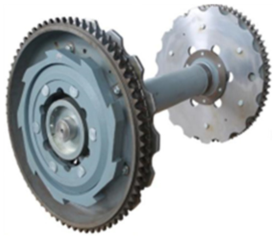
Figure 2.
Escalator main drive shaft.
Based on the Internet of Things (IoT), the application of artificial intelligence (AI) to escalator fault diagnosis can extract more abstract and deeper features from the complex operation data and reveal the complex correlation between the data and the failure of escalator components. The autonomous learning capabilities of deep learning facilitate the automatic extraction of critical features for fault diagnosis, paving the way for innovative approaches in escalator fault detection [6]. In the early stages, escalator faults typically exhibit subtle and weak symptoms that are difficult to detect through visual inspection. Sensors can capture subtle changes in the vibration of mechanical equipment and, by analyzing the signal characteristics, reveal the fault features and health status of mechanical components. Skog et al. [7] monitored the health status of elevator operation by converting vibration signals into spectrum and power spectrum, which helped detect and monitor equipment abnormalities through a frequency domain analysis. Xu Jinhai [8] utilized wavelet packet transformation and empirical mode decomposition to monitor and extract vibration signal features of elevator gearboxes under normal and abnormal conditions, demonstrating the effectiveness of time–frequency analysis techniques in identifying safety risks in mechanical components. Hao Gaoyan [9] proposed a variational mode decomposition envelope spectrum analysis method with an improved fitness function to address the challenges in diagnosing and extracting fault features of escalator rolling bearings. Zhang Yi [10] employed an envelope spectrum demodulation method based on spectral kurtosis to extract impact signals of escalator bearing faults and combined it with a linear prediction model for pre-whitening to improve the signal-to-noise ratio of weak bearing fault signals.
Sun [11] applied deep autoencoders to motor fault diagnosis. Feng [12] utilized deep autoencoder networks to extract vibration signal features of mechanical equipment for training artificial neural networks. Wan [13] employed the wavelet packet theory to extract representative features from elevator vibration signals and used them as inputs for an LS-SVM model to classify faults. Meng Qingyu [14] proposed an escalator main drive shaft bearing fault diagnosis method based on EEMD-SVM. This method first extracts abnormal vibration signal features of bearings using empirical mode decomposition and then constructs a fault diagnosis model using support vector machines.
Although various methods have been applied to escalator fault diagnosis, there are still challenges in detecting weak signals in complex working environments. Therefore, further research on automated fault diagnosis methods that combine IoT technology, sensor technology, and advanced machine learning techniques is crucial for improving the accuracy and real-time performance of equipment health monitoring [15]. This article tries to conduct a thorough study of IoT technology, sensor technology, and the escalator main drive shaft bearing, and constructs the data acquisition and transmission system of the escalator main drive shaft bearing from the perception layer to the application layer. A fault diagnosis method for the escalator main drive shaft based on a deep autoencoder (DAE) and Bidirectional Long Short-Term Memory Network (BiLSTM) is proposed. This method combines the deep autoencoder for data compression with the bidirectional memory network, where the extracted features are fed into the BiLSTM for accurate fault diagnosis and early warning.
The remainder of this paper is organized as follows: Section 2 introduces the algorithmic foundations, including autoencoders and LSTM networks. Section 3 presents the construction of the fault diagnosis model. Section 4 discusses the acquisition and transmission of the state data. Section 5 evaluates the proposed method through experiments and analysis.
2. Algorithmic Foundations
2.1. Brief Introduction to Autoencoder
The autoencoder learns the hidden layer feature [16] of multidimensional information through an unsupervised approach, and its structure is shown in Figure 3. The encoder contains both input and hidden layers, and the decoder consists of hidden and output layers. The encoding process [17] refers to the dimensional reconstruction of the input high-dimensional vibration signal through a nonlinear method so that the neural network can learn the most informative fault features; the decoding process refers to converting the vector of the hidden layer into an output vector with the same dimension of the input information by the non-linear method. Through the unsupervised learning method, the autoencoder extracts the fault features of the vibration signal, and its output can also be directly used as the input of the subsequent neural network training process.
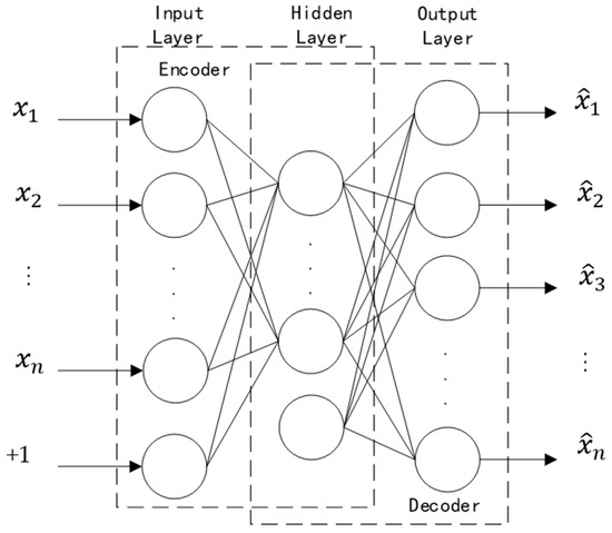
Figure 3.
Basic structure of the autoencoder [18].
2.2. The Principle of the Autoencoder
The definition of the autoencoder is briefly introduced as shown in Equations (1)–(6), which is fully researched in other research works [19]. Assuming that the input vector of the input layer is , the encoding vector of the hidden layer is , the output layer vector is , n is the dimension of the input and output vector, and m is the vector dimension of the hidden layer. For the input vector , the autoencoder is mapped to the hidden layer through the activation function with the following formula:
in which is the activation function, is the weight matrix of the encoder, is the bias item of the encoder, and (1) is the layer number.
The subsequent mapping function then maps the feature expression of the hidden layer into a reconstructed output vector . The vector is expressed as follows:
in which is the weight matrix of the decoder, is the biasing item of the decoder, and (2) is the layer number. Usually, the transpose of equal to is called the bundled weights, which can prevent the encoder from oversetting.
The activation function of the coding process and the decoding process adopts the sigmoid function, and the sigmoid form is as follows:
Since the value domain of is between 0 and 1, the input data are normalized.
The purpose of training the autoencoder is to minimize the reconstruction error between the input data and the output from the decoder. The formula of the loss function that defines the autoencoder is as follows:
in which the first term to the right of the equal sign represents the reconstruction error, where represents the number of training samples; the second term is the regularization term to prevent the model from oversetting, and represents the regularization coefficient.
In training the autoencoder, the network parameters are first initialized, and then the input data are passed through the forward propagation process layer by layer. This involves calculating the outputs of each layer’s neurons through activation functions, ultimately producing the overall output of the network. The weights and biases of each iteration are updated by gradient descent during error backpropagation, ensuring gradual convergence, while gradient clipping and weight clipping are applied to maintain training stability. The update equations for the weights and bias are shown in the following formula:
in which l is the number of iterations.
This architecture leverages the unsupervised feature extraction capability of DAE to remove noise and reduce the dimensionality of the input data, enabling BiLSTM to focus on critical temporal features. BiLSTM’s bidirectional learning captures both past and future states of the sequence, which is essential for identifying the gradual evolution of faults in machinery. The training process of the autoencoder can be represented by the flowchart shown in Figure 4.
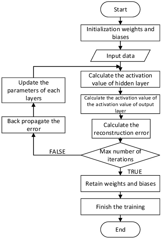
Figure 4.
The flowchart of the autoencoder training process.
2.3. Deep Autoencoder
In deep learning, there are generally many layers of neural network, and the model is relatively complex. Gradient descent is used to train the neural network. In the underlying network, gradient dispersion will appear, and the training difficulty will also increase. The deep autoencoder consists of multiple encoders, builds a stack autoencoder network, and has multiple hidden layers. Each layer of the autoencoder consists of an encoder–decoder pair connected through a “Code” layer, which represents the compressed data. The error transmission mechanism ensures that the reconstructed output retains essential information, minimizing the loss during the dimensionality reduction process. This layered configuration enables more robust feature representation, which is critical for tasks involving anomaly detection or data denoising. Compared with the autoencoder, the deep autoencoder network can better perform feature extraction [20], and its structure is shown in Figure 5.
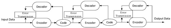
Figure 5.
Deep autoencoder structure.
Because the hidden layer reduces the dimensions of the input data, it cannot retain all features, leading to information loss during the encoding process. Training aims to minimize the loss of important features from the input data. In deep autoencoders, sparsity constraints are imposed on each layer, and multiple autoencoders are combined. During the training of the deep autoencoder network, a greedy layer-wise training approach is used. The training starts with the first layer of the network, where the hidden features learned by the layer are used as the input for the next layer. This layer-wise training strategy allows the model to focus on one level of representation at a time, avoiding issues such as vanishing gradients. The learned features from each layer are not only compact but also semantically meaningful, supporting the overall training stability. Once the first layer is trained, the process moves to the next layer, continuing in this layer-wise manner until all layers have been trained. Each layer is trained independently in an unsupervised fashion, ensuring that the model learns useful feature representations step by step. The model of the deep autoencoder is shown in Figure 6.
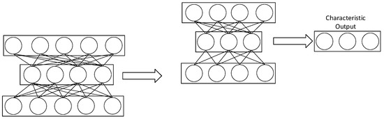
Figure 6.
Deep autoencoder mode.
2.4. Brief Introduction to Long Short-Term Memory Network
Long Short-Term Memory (LSTM) networks were developed as an improvement over recurrent neural networks (RNNs). RNNs learn and propagate historical information through time using backpropagation through time (BPTT). However, RNNs struggle with long time series due to the issues of vanishing and exploding gradients. Vanishing gradients prevent the earlier layers of the network from being updated properly, while exploding gradients can cause numerical instability during training. These gradient-related issues significantly limit the performance of RNNs on long time series tasks. LSTMs were designed to mitigate these problems, allowing for better handling of long-term dependencies [21]. As a deep learning model for improving recurrent neural networks, LSTM has the advantages of RNN to effectively learn non-linear features of time series, reflecting the temporal characteristics between data.
The memory unit of LSTM consists of four fully connected parts [22], consisting of the input gate, output gate, hidden layer, and forgetting gate. The LSTM network structure diagram is shown in Figure 7 [23]. The input gate multiplies with the input information, the output gate multiplies with the cell state, and the forgetting gate multiplies with the previous memory information, restricting the information values between 0 and 1. This operation acts as a ‘switch’ mechanism: if the product is close to 1, it allows information to pass through; if the product is close to 0, the information is blocked or ignored.
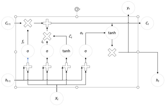
Figure 7.
LSTM network structure.
In Figure 7, is the state of the hidden layer at time t, is the state of the memory cell at time t, is the output from the previous time step, is the cell state from the previous time step, is the candidate value used for updating, are the input data at time t, represents the forgetting gate, represents the renewal gate, represents the output gate, represents the Sigmoid function, and tanh represents the hyperbolic tangent function.
The input of the LSTM includes the input value of the current moment and the state of the network at the previous moment, which flow through the forgetting gate, input gate, hidden layer and output gate, respectively. As for which information is saved and which information is forgotten, which is the result of the network optimization selection, the training of the neural network is actually the result of the optimization selection of the defined error function. LSTM has the transfer function and threshold as the traditional neuronal nodes, but the transfer function of the three gates takes a special sigmoid function.
3. Model Construction for Fault Diagnosis
3.1. Bidirectional Long Short-Term Memory Network
The gating mechanism of LSTM enables it to store long-term memory, but the information contained in the last state of LSTM often lacks completeness [24]. In one-way learning, LSTM has insufficient ability to learn the advanced information features and cannot effectively use the backward information, which affects the accuracy of the model. When diagnosing a main drive shaft bearing fault, both the condition of the parts before and after the failure is reflected in the subsequent vibration data, so the feature learning after the fault is also very necessary.
Based on the forward-learning LSTM, the Bidirectional Long Short-Term Memory Network (BiLSTM) adds the backward-learning LSTM [25]. BiLSTM is a neural network that can recurse the past and future hidden layer information of the current state. By connecting the past and future fault state information, the network can not only improve the utilization of data, but also improve the accuracy of the model. The BiLSTM network structure is shown in Figure 8.
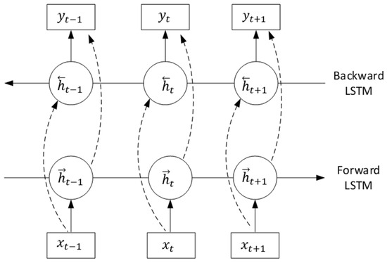
Figure 8.
BiLSTM network structure.
The forward calculation of the BiLSTM network can be described as follows:
where is the input at time t; is the input weight of the forward LSTM layer; is the weight of the forward LSTM layer at time t − 1; is the bias of the forward LSTM layer; is the adopted activation function; and is the forward calculation hidden vector of the forward LSTM layer.
The backward calculation of the BiLSTM network can be described as follows:
where is the input at time t; is the input weight of the backward LSTM layer; v is the weight of the backward LSTM layer at time t − 1; is the offset of the backward LSTM layer; and is the forward calculation hidden vector of the backward LSTM layer.
The output expression for the hidden layer is as follows:
where is the output of the hidden layer, which is synthesized from the output value of the forward hidden layer at each moment and the output value of the backward hidden layer at each moment.
3.2. Construction of the Fault Diagnosis Model for the Main Drive Shaft Bearing
A deep autoencoder (DAE) can learn the fault features in the sample of bearing vibration signals and restore the original signal through these features. After the DAE model training, the bearing vibration signal samples are dimensionally reconstructed according to the learning results as input information for the BiLSTM network. The BiLSTM learns the fault features in the vibration signal through the forward and backward hidden layers, so as to improve the diagnosis accuracy of the model. Using the vibration characteristics of the BiLSTM network before and after the occurrence of related faults, it can effectively learn the characteristic information of spindle-bearing vibration data and establish a reliable fault diagnosis model for early warning. In practical application, the model, on the one hand, can combine sensing data for real-time fault diagnosis; on the other hand, by identifying abnormal signals, it can infer that components may be in abnormal work or early fault state, to timely send out warning information and remind managers to pay attention to them.
The workflow of troubleshooting and warning of the main drive shaft bearing through the DAE-BiLSTM model is shown in Figure 9. First, the DAE network is constructed to determine the coding dimension of the hidden layer. The data set is input into the DAE model for training through the encoder and the decoder. The effect of the model training is verified by comparing the changes of the reconstruction error curve. After the training, the encoder is retained, and the training sample is reconstructed for dimensions. Secondly, the BiLSTM network is built to set the parameters of the model, including the number of samples, batch size, and number of hidden layer neurons. The reconstructed data of DAE network encoder were input into the BiLSTM network for learning and training. After the training, the diagnostic effect of the model was evaluated with the validation set, the best parameters of the model were used to obtain the grid search method, and finally the fault diagnosis model of the key components of the escalator was obtained. The specific process is as follows:
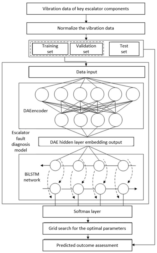
Figure 9.
Main drive shaft fault diagnosis frame diagram.
- DAE Model Training
Step 1: Obtain the training sample. Use the vibration sensor to collect the vibration information of the main drive shaft bearing of the escalator.
Step 2: Preprocess the input samples. The raw vibration signal samples were normalized, and the normalization formula was expressed as follows:
Step 3: Divide the data set. In the process of learning, the data set is usually divided into three parts: the training set, validation set, and test set. The training set is used for model setting, where gradient descent is applied to the training error to adjust the weights and biases of the network; the validation set is used to adjust the hyperparameters of the model to prevent oversetting and evaluate the model performance; and the test set is used to evaluate the diagnostic effect of the model. In this paper, the data set is divided into the training set, the verification set, and the test set, according to the proportion of 7:2:1.
Step 4: DAE model training. Enter the bearing vibration sample into the DAE model, set the parameters such as the model training number and hidden layer cell number, and initialize the weight matrix W and bias vector b. First, perform forward propagation to obtain the output value; then, update the weights and bias of the network through error backpropagation. After training the DAE model, the encoder part is retained, and the vibration signal sample data are reconstructed.
- 2.
- BiLSTM Fault Diagnosing
Step 1: Input the hidden layer output (embedding) of the DAE network into the BiLSTM network. The BiLSTM network processes the dimensionally reconstructed vibration information from the main drive shaft bearing, using forward and backward layers to extract past and future hidden information. Specifically, the forward layer processes the information sequentially from the past to the present, while the backward layer processes the information in reverse, from the future to the present. Through this bidirectional processing, the network learns the patterns of different fault vibration signals, calculates the forward and backward outputs separately, and then sums them to produce the final output of the BiLSTM hidden layer.
Step 2: connect the Softmax network layer, obtain the prediction probability matrix according to the output of the hidden layer, and classify the fault vibration samples.
Step 3: by iteratively training and optimizing the network model using the gradient descent algorithm to minimize the cross-entropy loss between the actual and theoretical outputs, the best network parameters are selected, thereby enabling more accurate fault diagnosis of the main drive axis.
Step 4: test the data by inputting them into the model and use the cross-entropy loss as the evaluation metric to assess the diagnostic effect of the model.
4. State Data Acquisition and Transmission of the Main Drive Shaft Bearing
The sensing layer of the bearing data acquisition and transmission system of the main drive shaft of the escalator obtains the operation status data of the main drive shaft of the escalator through the sensor network, and the data collector sends the power or non-power signals collected from the sensor and other underlying equipment to the upper machine. The transmission layer sends the data to the application layer through the network transmission technology and saves the data analysis in the database.
In this article, the piezoelectric vibration acceleration sensor SE830 is suitable to collect the running state change data of the main drive shaft of the escalator. All the parameters are shown in Table 1. The piezoelectric acceleration sensor is suitable for measuring the absolute movement of the bearing seat, reducer housing, foundation, etc. The frequency range that can be measured is 0.2 Hz~20 kHz, which is usually used for measuring the high frequency vibration signal of motor and high speed caused by bearing damage.

Table 1.
Parameter index of the vibration acceleration sensor.
The position of the monitoring point and the installation mode of the sensor will affect the accuracy of the collected vibration signal. To ensure stable and secure contact between the vibration sensor and the measured parts during the measurement process, the system uses a magnet to attach the vibration sensor to the bearing seat of the main drive shaft. The raw vibration signals collected may contain errors due to various environmental factors. One common issue is the presence of trend components, where the vibration signal gradually deviates from the baseline over time. To address this, the least squares method is employed to remove the trend from the signal. Digital filtering is also a crucial step in signal processing. A digital filter is a discrete-time system that transforms the input signal into the desired discrete-time or numerical signal according to a predefined algorithm. In this study, a Butterworth filter was selected for the filtering module due to its well-balanced performance in both amplitude and phase characteristics.
The data collector receives the data sent by the sensor, and it needs to send the data to the application layer server through the communication transmission technology. Network layer communication technology develops rapidly and has many types, mainly including Ethernet, 3G/4G, WIFI, NB-IoT, etc. The advantages and disadvantages of various communication technologies are summarized as shown in Table 2.
Table 2.
Comparison of the Internet of Things transmission technology characteristics.
The data acquisition and transmission system of the main drive shaft bearing of the escalator has the following characteristics:
- High frequency vibration signal sampling;
- The complex internal environment of the escalator leads to signal instability.
Wireless signals generated by communication devices such as passenger mobile phones interfere with data transmission, and wireless communication technology is not compatible with data transmission on escalators. Considering the large amount of data generated by the long operation of the escalator, there are high requirements for the transmission rate and data capacity. After analysis and comparison, Ethernet is more suitable to meet the needs of escalator data acquisition and transmission system. The data are transmitted to the local server through Ethernet. The information transmission format mainly includes five parts: the start code, device code, data collection, check code, and end code. The number and content of each field are shown in Table 3.
Table 3.
Data format.
In this article, the Block Check Character is used to detect the data. When the data are sent and received, all the data in the field will be calculated to obtain the verification code, and the verification code will be compared. If the data are equal, it means that the data are effective, otherwise the data are abandoned.
The specific process of data storage is that after the server receives the data, the corresponding fields according to the data format to form a log file temporarily exists locally. The system reads the log file by regularly triggering events and saves the data in the database. The system selects the simple and easy to operate Navicat2023 software to add, delete, change, and check the database.
5. Bearing Fault Diagnosis, Verification, and Analysis
5.1. Experimental Data and Parameter Settings
- Acquisition of Training Data
In university experiments, conducting extensive tests on both normal and damaged bearings is costly and challenging. Although we have established a detailed data acquisition process and collected some bearing-related data, this paper uses the bearing acceleration data from the Bearing Data Center at Case Western Reserve University (CWRU) as the training set, enabling the model to accurately identify bearing fault types. The bearing faults included in this data set exhibit significant relative damage and distinct fault features, making diagnosis easier. Additionally, since bearings share similar vibration characteristics, the long short-term neural network can fully capture their fault characteristics.
The experiments were implemented using Python 3.8, with PyCharm as the development environment, and the TensorFlow and Keras libraries for the model construction and training.
To enhance the robustness and generalization ability of the training model, the sliding window is used to enhance the data [26] of the vibration signal by overlapping sampling; following the method of generating sample data as shown in Figure 10, set the sliding window by dividing the sample signal, and move the window according to the specified step size for the next sampling. Overlap between samples occurs when the sliding step of the window is smaller than the length of a single sample. This article set the sliding window size to 1024 and the fixed moving step size to 28.
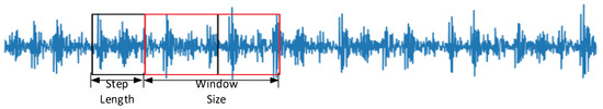
Figure 10.
A Schematic representation of the data augmentation.
- 2.
- Data Preprocessing
The samples were normalized and mapped to the [0,1] interval. The normalized sample data were then divided into 70% as the training set, 20% as the validation set, and 10% for the test set. The number of samples and labels for each failure mode are shown in Table 4.
Table 4.
Number of samples for different faults.
- 3.
- Set the parameters of the DAE model
The DAE network parameters were first set, and the vibration signal samples were input for training. The role of each parameter is explained in the following: ① Learning rate: The learning rate affects the model’s convergence speed. A low learning rate can prolong training and cause oversetting, while a high learning rate may lead to unstable training and poor model performance. ② Batch processing: by dividing the training set into equal data batches, the training process can leverage parallelization to reduce the resource consumption and accelerate the training speed, while also facilitating the implementation of other optimized training strategies. ③ Activation function: ssing ReLU activation function in the DAE network can not only reduce the calculation amount of back propagation, but also reduce the dependence between connection weights and reduce the possibility of oversetting. ④ Output layer function: select the Sigmoid function, and the normalized data can be restored during the decoding process. ⑤ Loss function: select MSE, which has a good effect when evaluating the deviation between the input and output. ⑥ Optimizer: The optimizer can affect the efficiency of model training. During the training process, the stochastic gradient descent algorithm keeps a single learning rate unchanged when updating the weights, while the Adam optimizer training is stable and faster, and can adaptively adjust different learning rates, so the Adam algorithm is selected for the optimizer training. The specific parameters of the DAE model are shown in Table 5.
Table 5.
DAE network parameter.
The loss rate curves for the DAE training and validation sets are shown in Figure 11. After 300 training iterations, the loss function stabilizes, indicating that the model has converged. Following the encoder’s encoding process, the original sample data is reconstructed into 400-dimensional data. Additionally, we used the validation set to adjust the model’s hyperparameters and prevent overfitting. The integration of DAE significantly reduces the input dimensionality, which lowers the computational burden for BiLSTM while maintaining a high level of diagnostic accuracy. In addition, the denoising effect of DAE enhances the robustness of the model in real-world scenarios, allowing BiLSTM to process more reliable and fault-related features even in the presence of substantial background noise. Generally, the activation function and loss function for the autoencoder are ReLU and MSE, respectively. Regarding parameter selection, there is no fixed standard for choosing the number of layers and the dimensionality of each layer in a deep autoencoder. The layer-by-layer greedy training approach allows the pre-trained network to approximate the structure of the original data to some extent, enabling the network to obtain appropriately tuned feature values and facilitating faster convergence during the supervised training phase.
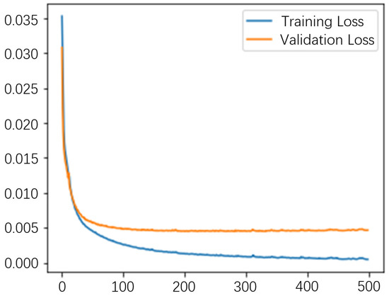
Figure 11.
DAE training set validation set loss function.
- 4.
- BiLSTM parameter setting
Factors influencing the training results of the BiLSTM network include the parameter selection, such as the number of BiLSTM cells, optimizer, and learning rate. The number of hidden layer cells represents the number of nodes used for memory and storage states, and the number of cells affects the diagnosis speed and accuracy. Since there are many similar parameters between the BiLSTM network and DAE network, it will not be described here. If the BiLSTM network parameters are as shown in Table 6, the number of cells of BiLSTM is set as 64, the learning rate is set to 0.001, the activation function is “tanh”, the training number is 200, and the probability of the inactivation of dropout neurons is 0.2.
Table 6.
BiLSTM network parameters.
The compressed representation of the input data generated by the DAE network is input into the BiLSTM network, and then, the processing results of the BiLSTM network are passed to the Softmax layer, where the output layer dimension matches the final number of classifications. The Adam optimizer will keep updating the network parameters based on the loss function, and finally, the fault diagnosis model of the main drive shaft bearing can be obtained.
5.2. Experimental Results and Analysis
The accuracy and loss rate curves for the training and validation sets of the bearing fault diagnosis model are shown in Figure 12. It can be observed from the accuracy curve that the training accuracy of the model is low due to the random setting of the BiLSTM network. However, with the number of training times, the recognition accuracy of the model improved rapidly, over 99%. After 150 training iterations, the accuracy of the model approached 100% and stabilized. The loss rate curve of the training set shows that the loss rate fluctuated greatly in the first 25 training iterations, but the fluctuation amplitude of the loss curve gradually decreased with the training number, and the loss rate finally stabilized and approached 0 after 150 trains. This shows that the diagnostic accuracy of the fault state improves significantly with continuous network learning. Figure 13 illustrates the diagnostic outcome confusion matrix for the bearing test set. The results show that the model can effectively identify the normal fault of the bearing, the main drive shaft, and the outer ring.
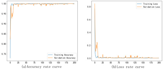
Figure 12.
Accuracy and loss rate curve of the fault diagnosis model.
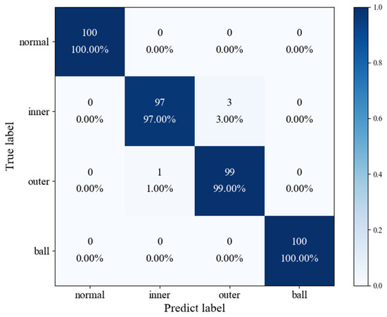
Figure 13.
Confusion matrix based on the DAE-BiLSTM fault diagnosis.
To verify the superiority of this method, the same batch size, learning rate, and other parameters were selected, and the DAE-BiLSTM method was compared with the method using only BiLSTM. The BiLSTM model parameters are set as follows: the number of cells in the input layer is 1024, the number of cells in the forward and backward hidden layers is 64, the activation function selects tanh, and finally goes through the softmax layer classification.
The accuracy curve of the DAE-BiLSTM and BiLSTM models is shown in Figure 14. Table 7 shows the comparison of the training time of the two models. The DAE-BiLSTM method changed greatly in the first 12 iterations, and the model converged; however, the training speed is fast and quickly reached a stable state, and the accuracy reached more than 99%. With increasing training times, the accuracy curves of the two models coincide, and the DAE-BiLSTM model has a shorter training time.
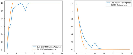
Figure 14.
Accuracy and loss rate curves of the training sets for the different models.
Table 7.
The diagnostic comparison of the different models.
From the above results, we can see that the proposed DAE-BiLSTM model is close to the BiLSTM model. However, the DAE-BiLSTM model achieves dimensional reconstruction through a deep autoencoder, squeezing the 1024-dimensional input vibration information down to 400 dimensions. While retaining the necessary fault feature information, this dimensional compression reduces the computational cost of the BiLSTM significantly, and reduces the training time of the BiLSTM, thus greatly shortening the training time of the model. In comparison, Xia [27] proposed a CNN-based fault diagnosis method for rotating machinery using multi-sensor fusion, achieving 99.41% accuracy with two sensors and 98.35% with one. Although the CNN method offers a high accuracy, it does not explicitly address dimensionality reduction or the computational efficiency of training. Shao [28] employed an adaptive DBN with DTCWPT for preprocessing raw vibration signals, achieving 94.37% accuracy. Their method involves multiple preprocessing techniques and a complex network architecture, which may lead to an increased computation and training time. Zhou [29] proposed a fault diagnosis method using global optimization GAN, which integrates DNN feature extraction with GAN’s data generation capabilities. This approach, while achieving good diagnostic accuracy (94.58%, 96.85%, and 93.28% for inner-race, roller, and outer-race faults), relies on adversarial training and sample generation.
6. Conclusions
This paper introduces an innovative escalator condition monitoring and early warning system that combines IoT technology, sensor technology, and fault diagnosis methods, employing a deep autoencoder (DAE) and Bidirectional Long Short-Term Memory (BiLSTM) network model for fault detection.
The proposed approach first utilizes the DAE to compress and extract key features from the input vibration signals, which are then fed into the BiLSTM network for fault diagnosis. The results demonstrate that the DAE-BiLSTM model can accurately detect faults in the inner and outer rings as well as the rolling elements of bearings, achieving a diagnostic accuracy of over 99%. Compared to the standalone BiLSTM model, the DAE-BiLSTM method significantly reduces the training time through data compression while enhancing the diagnostic efficiency and model generalization. By installing sensors on critical components, the system enables the precise monitoring of escalator operating conditions, and through the use of Ethernet technology, ensures high-security and high-reliability remote data transmission.
Furthermore, the research presented in this paper offers valuable insights for the informatized management of escalator maintenance, helping to quickly detect anomalies to prevent potential failures. However, this study has some limitations. The model is primarily based on data from bearing faults, and further research is needed to validate its performance with other types of faults in different components. Additionally, the system’s effectiveness may be influenced by the quality and variety of sensor data, and improvements in data acquisition could enhance the model accuracy and robustness. Future research should expand to cover other transmission components, such as tensioning shafts and main drive chains, to achieve the comprehensive monitoring and fault diagnosis of the entire escalator system.
Author Contributions
Conceptualization, Y.T.; data curation, X.J. and Z.Z.; formal analysis, H.Y.; investigation, X.J.; methodology, H.Y.; software, X.J. and Z.Z.; validation, J.H. and Y.T.; writing—original draft, X.J. and Z.Z.; writing—review and editing, J.H. and Y.T. All authors have read and agreed to the published version of the manuscript.
Funding
This research was funded by Program of Science Foundation of Jiangsu Province Special Equipment Safety Supervision Inspection Institute (No. KJ(Y)2023034).
Data Availability Statement
The data presented in this study are openly available in the Case Western Reserve University Bearing Data Center at https://engineering.case.edu/bearingdatacenter/download-data-file (accessed on 31 July 2024).
Acknowledgments
This work was financially supported by Program of Science Foundation of Jiangsu Province Special Equipment Safety Supervision Inspection Institute (No. KJ(Y)2023034). We also appreciate the Case Western Reserve University Bearing Data Center for providing the data for this study. Finally, we express our gratitude to the reviewers for their constructive comments, which helped to improve the quality of this manuscript.
Conflicts of Interest
The authors declare no conflicts of interest.
References
- Vasily, O.; Nataly, Z.; Alexey, S. Intelligent escalator passenger safety management. Sci. Rep. 2022, 12, 5506. [Google Scholar]
- Xing, Y.; Chen, S.; Zhu, S.; Lu, J. Analysis Factors That Influence Escalator-Related Injuries in Metro Stations Based on Bayesian Networks: A Case Study in China. Int. J. Environ. Res. Public Health 2020, 17, 481. [Google Scholar] [CrossRef] [PubMed]
- Fan, J. On the importance of intelligent video surveillance system to improve the safety of escalator riding. China Elev. 2022, 33, 40–43. [Google Scholar]
- Chen, J.; Zhang, Z. Research on escalator data acquisition and transmission based on big data platform. Procedia Comput. Sci. 2022, 208, 532–538. [Google Scholar] [CrossRef]
- You, F.; Wang, D. Fault diagnosis method of escalator step system based on vibration signal analysis. Int. J. Control Autom. Syst. 2022, 20, 3222–3232. [Google Scholar] [CrossRef]
- Brito, L.C.; Antonio, G.S. An explainable artificial intelligence approach for unsupervised fault detection and diagnosis in rotating machinery. Mech. Syst. Signal Process. 2022, 163, 108–121. [Google Scholar] [CrossRef]
- Skog, I.; Karagiannis, I.; Bergsten, A. A Smart Sensor Node for the Internet-of-Elevators-Non-Invasive Condition and Fault Monitoring. IEEE Sens. J. 2017, 17, 5198–5208. [Google Scholar] [CrossRef]
- Xu, J.H.; Xu, L.; Wang, H. Research on Elevator Condition Monitoring Technology Based on Vibration Analysis. Electromech. Eng. 2019, 36, 279–283. [Google Scholar]
- Zhang, Y.; Hao, G.Y.; Liu, X. Application of Improved Variational Mode Decomposition Envelope Spectrum Analysis in Escalator Bearing Fault Diagnosis. Bearing 2021, 46–51. [Google Scholar] [CrossRef]
- Zhang, Y.; Hao, G.Y.; Liu, X. Application of Envelope Demodulation Method in Escalator Bearing Fault Diagnosis. Equip. Manag. Maint. 2021, 152–154. [Google Scholar]
- Sun, W.; Shao, S.; Zhao, R.; Yan, R.; Zhang, X.; Chen, X. A parse auto-encoder-based deep neural network approach for induction motor faults classification. Measurement 2016, 89, 171–178. [Google Scholar] [CrossRef]
- Jia, F.; Lei, Y.; Lin, J.; Zhou, X.; Lu, N. Deep neural networks: A promising tool for fault characteristic mining and intelligent diagnosis of rotating machinery with massive data. Mech. Syst. Signal Process. 2016, 72–73, 303–315. [Google Scholar] [CrossRef]
- Wan, Z.; Yi, S.; Li, K.; Tao, R.; Gou, M.; Li, X.; Guo, S. Diagnosis of elevator faults with LS-SVM based on optimization by K-CV. J. Electr. Comput. Eng. 2015, 33, 935038. [Google Scholar] [CrossRef]
- Meng, Q. Research on escalator main drive shaft bearing fault diagnosis method based on EEMD-SVM. Mech. Electr. Eng. 2020, 38, 51–53, 58. [Google Scholar]
- E, X.; Wang, W. Escalator Foundation Bolt Loosening Fault Recognition Based on Empirical Wavelet Transform and Multi-Scale Gray-Gradient Co-Occurrence Matrix. Sensors 2023, 23, 6801. [Google Scholar] [CrossRef]
- Li, P.; Pei, Y. A comprehensive survey on design and application of autoencoder in deep learning. Appl. Soft Comput. J. 2023, 138, 109412. [Google Scholar] [CrossRef]
- Ren, J.; Ni, D. A batch-wise LSTM-encoder decoder network for batch process monitoring. Chem. Eng. Res. Des. 2020, 164, 102–112. [Google Scholar] [CrossRef]
- Yann, L.C.; Françoise, F.S. Modèles connexionnistes de l’apprentissage. Intellectica Rev. L Assoc. Pour Rech. Cogn. 1987, 2–3, 114–143. [Google Scholar]
- Goodfellow, I.; Bengio, Y. Deep Learning, 1st ed.; MIT Press: Cambridge, MA, USA, 2016; pp. 499–507. [Google Scholar]
- Tong, J.; Luo, J. Fault diagnosis method of rolling bearing based on enhanced deep auto-encoder network. China Mach. Eng. 2021, 32, 45–51. [Google Scholar]
- Ravikumar, A.; Sriraman, H. A Deep Understanding of Long Short-Term Memory for Solving Vanishing Error Problem: LSTM-VGP. In Machine Learning Algorithms Using Scikit and TensorFlow Environments; IGI Global: Hershey, PA, USA, 2024; pp. 74–90. [Google Scholar]
- Sha, X.J. Time series stock price forecasting based on genetic algorithm (GA)-long short-term memory network (LSTM) optimization. arXiv 2024, arXiv:2405.03151. [Google Scholar] [CrossRef]
- Lui, C.F.; Liu, Y.; Xie, M. A supervised bidirectional long short-term memory network for data-driven dynamic soft sensor modeling. IEEE Trans. Instrum. Meas. 2022, 71, 2504713. [Google Scholar] [CrossRef]
- Siami-Namini, S.; Tavakoli, N.; Namin, A.S. The performance of LSTM andBiLSTM in forecasting time series. In Proceedings of the 2019 IEEE International Conference on Big Data (Big Data), Los Angeles, CA, USA, 9–12 December 2019; IEEE: Piscataway, NJ, USA, 2019; pp. 3285–3292. [Google Scholar]
- Chen, C.; Lu, N.; Jiang, B. Prediction interval estimation of aeroengine remaining useful life based on bidirectional long short-term memory network. IEEE Trans. Instrum. Meas. 2021, 70, 1–13. [Google Scholar] [CrossRef]
- Meng, Z.; Guan, Y.; Pan, Z.; Sun, D.; Fan, F.; Cao, L. Fault diagnosis of rolling bearing based on secondary data enhancement and deep convolutional network. J. Mech. Eng. 2021, 57, 106–115. [Google Scholar]
- Xia, M.; Li, T.; Xu, L.; Liu, L.; de Silva, C.W. Fault diagnosis for rotating machinery using multiple sensors and convolutional neural network. IEEE/ASME Trans. Mechatron. 2018, 23, 101–110. [Google Scholar] [CrossRef]
- Shao, H.; Jiang, H.; Wang, F.; Wang, Y. Rolling bearing fault diagnosis using adaptive deep belief network with dual-tree complex wavelet packet. ISA Trans. 2017, 69, 187–201. [Google Scholar] [CrossRef]
- Zhou, F.; Yang, S.; Fujita, H.; Chen, D.; Wen, C. Deep learning fault diagnosis method based on global optimization GAN for unbalanced date. Knowl.-Based Syst. 2020, 187, 104837. [Google Scholar] [CrossRef]


Disclaimer/Publisher’s Note: The statements, opinions and data contained in all publications are solely those of the individual author(s) and contributor(s) and not of MDPI and/or the editor(s). MDPI and/or the editor(s) disclaim responsibility for any injury to people or property resulting from any ideas, methods, instructions or products referred to in the content. |
© 2025 by the authors. Licensee MDPI, Basel, Switzerland. This article is an open access article distributed under the terms and conditions of the Creative Commons Attribution (CC BY) license (https://creativecommons.org/licenses/by/4.0/).