Fuzzy Control of Multivariable Nonlinear Systems Using T–S Fuzzy Model and Principal Component Analysis Technique

Abstract

In this work, a new nonlinear control method is proposed, which integrates the Takagi–Sugeno (T–S) fuzzy model with the Principal Component Analysis (PCA) technique. The approach uses PCA to reduce the system’s dimensionality, minimizing the number of fuzzy rules required in the T–S fuzzy model. This reduction not only simplifies the system variables but also decreases the computational complexity, resulting in a more efficient control with smooth transient responses and zero steady-state error. To validate the performance of this PCA-based approach for both system identification and control, an interconnected double-tank system was employed. The results demonstrate the method’s capacity to maintain control accuracy while reducing computational load, making it a promising solution for applications in industrial and engineering systems that require robust, efficient control mechanisms.

1. Introduction

Traditional control methodologies often face significant challenges when applied to complex and nonlinear systems. Among these challenges are the difficulty in accurately modeling system dynamics, the computational cost associated with handling high-dimensional data, and the lack of robustness in noisy environments. These limitations have prompted the exploration of alternative approaches that can effectively overcome these problems while maintaining simplicity and adaptability. In this context, the PCA technique applied in fuzzy control is presented as a powerful tool that offers robust and adaptive solutions for nonlinear systems in the presence of disturbances, load and noise effects.

Fuzzy control, based on fuzzy logic [1], proposes a robust and adaptive alternative to solve control problems where rules and relationships are not easily defined with traditional methods. In [2], an approach developed by the authors is presented to apply fuzzy logic for the identification and control of a double-tank system. This approach demonstrates the effectiveness of fuzzy methodologies in identifying nonlinear systems. The research provides a solid foundation for future applications of fuzzy logic in modeling and controlling complex industrial systems.

Another approach was developed in [3], applying a fuzzy adaptive sliding mode control to hydraulic servo systems. This method aimed to enhance robustness and adaptability by integrating fuzzy logic to handle system nonlinearities and parameter uncertainties, achieving superior performance in tracking accuracy and stability under external disturbances. In [4], a similar fuzzy adaptive sliding mode controller was applied to an electronic throttle control system, addressing the nonlinear dynamics and time-varying parameters inherent in such systems. The adaptive nature of the fuzzy controller ensured real-time adjustment of control gains, improving both transient and steady-state responses.

One of the advantages in fuzzy logic is its integration with Proportional, Integral and Derivative (PID) controllers, a strategy that has been explored in different applications [5,6,7]. The authors propose a fuzzy-PID hybrid controller for optimizing the performance of different systems, such as wind turbines [5], power plant [6] and voltage regulator [7].

Based on fuzzy-PID control advances, the use of fuzzy logic with Linear Quadratic Regulator (LQR) control has emerged as a significant development due to LQR’s advantages over traditional PID controllers. LQR provides optimal control performance by minimizing a cost function that balances control effort and system performance, which is particularly beneficial for complex systems. This approach has been successfully applied across various domains, such as anti-swing pendulums [8] and robotic systems [9]. By combining fuzzy logic with LQR, these systems benefit from enhanced stability, precision, and adaptability.

In [10], another approach is introduced, focusing on an incremental Takagi–Sugeno (T–S) state model for optimal control of multivariable nonlinear time-delay systems. This model offers significant advantages in handling complex dynamic systems with time delays, providing more precise control and adaptability. Similar incremental strategies have been applied in [11], where the method introduces an integral action, causing steady state errors to be canceled. Applications of this incremental model can also be found in the control of solar plants, as demonstrated in [12]. These studies highlight the versatility of the incremental approach in addressing complex real-world control challenges.

Despite the advantages of fuzzy control systems, they often have computational cost problems, particularly in high-dimensional systems where the complexity of rule-based models can grow exponentially. One of the main objectives of this work is to resolve this limitation by incorporating Principal Component Analysis (PCA) technique into the fuzzy control framework, reducing computational costs while maintaining or even improving performance.

The PCA technique has the ability to reduce the dimensionality of data, allowing the identification of patterns and simplifying the modeling of complex systems. PCA has been applied to image processing [13], traffic control systems [14], cybersecurity, [15], big data models [16] or medical purposes [17], where the authors propose a method that improves the efficiency of identifying key attributes.

The application of PCA in controllers has proven to be a valuable method to improve system performance through data reduction and pattern recognition. In [18], PCA is used to define fuzzy sets, followed by the implementation of an adaptive fuzzy controller in an intelligent drying system. A regression model is developed using PCA in [19], which is applied in predictive control to maintain the quality of plastic fabrication process. The integration of PCA with control strategies is further demonstrated in [20], where a fuzzy PID controller is enhanced by a PCA-based algorithm to regulate voltage in AVR systems. In addition, a predictive control model that uses PCA is explored in [21] for efficient energy management. Finally, in [22], a hybrid PCA and fuzzy PID control approach was applied to the cooling system of a power plant, optimizing sample identification and system response. These studies underscore PCA’s effectiveness in control systems across diverse applications.

In this work, the three approaches mentioned above will be used: fuzzy logic with LQR controller, incremental T–S state model, and PCA technique. Due to the use of these approaches, the fuzzy rules are perfectly adjusted to the achievable points in the output variables of the system, since certain points in the working range will not be achievable and it would be inefficient to place rules at these points. The objective is to apply the PCA technique in nonlinear systems to reduce the fuzzy rules without affecting the accuracy in the identification and control of the system and, in addition, reducing the computational cost.

The rest of this work is organized as follows. In Section 2, the T–S, model identification and control is described. The identification and control process using the PCA technique is presented in Section 3. In Section 4, the identification based on the T–S model and the PCA technique is used in an illustrative example of an interconnected double-tank system. In Section 5, an incremental controller is presented to show the advantages of the proposed T–S model based on PCA.

2. T–S Fuzzy Model Identification and Control

The T–S fuzzy model identification method proposes an estimation of the nonlinear parameters of the system minimizing a quadratic performance index [23]. The conventional T–S identification approach has limitations when triangular membership functions of fuzzy rules overlap in pairs, as the resulting T–S matrix is not of full rank and, therefore, cannot be inverted [24]. Therefore, the authors in [24] introduced a generalized T–S identification that employs a parameter weighting method.

The approach is based on the identification of nonlinear functions, which can be represented as a set of difference equations. These equations are formulated by using the following IF-THEN rules for an nth-order system:

$$\begin{array}{cc}\hfill S^{(i_1\dots i_m)}& : \mathrm{if} z_1\left(k\right) \mathrm{is} M_1^{i_1} \mathrm{and} \dots \mathrm{and} z_m\left(k\right)\mathrm{is} M_m^{i_m} \mathrm{then}:\hfill \\ \hfill y(k+1)& =a_0^{(i_1\dots i_m)}+a_1^{(i_1\dots i_m)}y\left(k\right)+\dots +a_n^{(i_1\dots i_m)}y(k-n+1)\hfill \\ \hfill & +b_1^{(i_1\dots i_m)}u\left(k\right)+\dots +b_n^{(i_1\dots i_m)}u(k-n+1)\hfill \\ \hfill & ⋮\hfill \end{array}$$

(1)

where system outputs are represented as $\{y_1\left(k\right),y_2\left(k\right),\dots y_s\left(k\right)\}$, while system inputs are denoted as $\{u_1\left(k\right),u_2\left(k\right),\dots u_p\left(k\right)\}$. The measurable variables, $\{z_1\left(k\right),z_2\left(k\right),\dots z_m\left(k\right)\}$, will hereinafter be referred to as fuzzy variables. Moreover, $M_j^{i_j}$ represents the fuzzy sets associated with the fuzzy membership functions ${\mu }_j^{i_j}\left(z_j\left(k\right)\right)$. In this fuzzy notation, j corresponds to the fuzzy variable index and $i_j$ is the fuzzy rule index associated with the fuzzy variable.

For the parameter weighting method, it is assumed that a first affine linear estimation model is available. In other words, an initial estimation of the parameters listed below is provided.

$$\begin{array}{c}\hfill P=\left[\begin{array}{ccccccc}{a}_0^0& a_1^0& \dots & a_n^0& b_1^0& \dots & b_n^0\end{array}\right]\end{array}$$

(2)

In order to obtain this first estimation, the classical least squares method can be applied to the data set of the system. This estimation can be used as a reference parameter for all subsystems of the fuzzy T–S model.

$$\begin{array}{c}\hfill p_0=\underset{r_1,r_2\dots r_m}{\underbrace{{\left[\begin{array}{cccc}{P}_0& P_0& \dots & P_0\end{array}\right]}^t}}\end{array}$$

(3)

The fuzzy model parameters can be obtained minimizing a quadratic performance index:

$$\begin{array}{cc}\hfill J& =\sum _{k=1}^{n_S}{(y\left(k\right)-\widehat{y}\left(k\right))}^2+{\gamma }^2\sum _{i_1=1}^{r_1}\dots \sum _{i_m=1}^{r_m}\sum _{j=0}^n{(p_j^0-p_j^{(i_1\dots i_m)})}^2\hfill \\ \hfill & ={\parallel Y-XP\parallel }^2+{\gamma }^2{\parallel p_0-P\parallel }^2\hfill \\ \hfill & ={∥\left[\begin{array}{c}Y\\ \gamma p_0\end{array}\right]-\left[\begin{array}{c}X\\ \gamma I\end{array}\right]P∥}^2={∥Y_a-X_{a}P∥}^2\hfill \end{array}$$

(4)

where Y represents the output data, X corresponds to the fuzzy input/output data and P denotes the parameters of the fuzzy model.

The factor $\gamma$ shows the degree of confidence in the parameters obtained from the initial estimation [24]. Note that the matrix $X_a$ has full rank, even if the triangular membership functions overlap in pairs. This solves the problem while the original T–S identification method fails. Thus, the vector P can be determined as follows:

$$\begin{array}{c}\hfill P={\left(X_a^t{X}_a\right)}^{-1}{X}_a^t{Y}_a\end{array}$$

(5)

Based on the discrete fuzzy system described above, the fuzzy rules can be reformulated into a state model, as detailed in [10].

$$\begin{array}{cc}\hfill S^{(i_1\dots i_m)}& : \mathrm{if} z_1\left(k\right) \mathrm{is} M_1^{i_1} \mathrm{and} \dots \mathrm{and} z_m\left(k\right) \mathrm{is} M_m^{i_m} \mathrm{then}:\hfill \\ \hfill x(k+1)& =a_x^{(i_1\dots i_m)}+A^{(i_1\dots i_m)}x\left(k\right)+B^{(i_1\dots i_m)}u\left(k\right)\hfill \\ \hfill y\left(k\right)& =a_y^{(i_1\dots i_m)}+C^{(i_1\dots i_m)}x\left(k\right)\hfill \\ \hfill & ⋮\hfill \end{array}$$

(6)

where $a_x\in R\left(nx1\right)$, $A\in R\left(nxn\right)$, and $B\in R\left(nxp\right)$, where p denotes the number of inputs and $C\in R\left(1xn\right)$. The matrices are defined as follows:

$$\begin{array}{cc}\hfill a_x^{(i_1\dots i_m)}=\left[\begin{array}{c}{a}_{x1}^{(i_1\dots i_m)}\\ a_{x2}^{(i_1\dots i_m)}\\ ⋮\\ a_{xn}^{(i_1\dots i_m)}\end{array}\right]& A^{(i_1\dots i_m)}=\left[\begin{array}{cccc}{A}_1^{(i_1\dots i_m)}& 0& \dots & 0\\ 0& A_2^{(i_1\dots i_m)}& \dots & 0\\ ⋮& ⋮& \ddots & ⋮\\ 0& 0& \dots & A_n^{(i_1\dots i_m)}\\ \end{array}\right]\hfill \\ \hfill B^{(i_1\dots i_m)}=\left[\begin{array}{c}{B}_1^{(i_1\dots i_m)}\\ B_2^{(i_1\dots i_m)}\\ ⋮\\ B_n^{(i_1\dots i_m)}\end{array}\right]& a_y^{(i_1\dots i_m)}=\left[\begin{array}{c}{a}_{y1}^{(i_1\dots i_m)}\\ a_{y2}^{(i_1\dots i_m)}\\ ⋮\\ a_{yn}^{(i_1\dots i_m)}\end{array}\right]\hfill \\ \hfill C^{(i_1\dots i_m)}=& \left[\begin{array}{cccc}{C}_1^{(i_1\dots i_m)}& 0& \dots & 0\\ 0& C_2^{(i_1\dots i_m)}& \dots & 0\\ ⋮& ⋮& \ddots & ⋮\\ 0& 0& \dots & C_n^{(i_1\dots i_m)}\\ \end{array}\right]\hfill \end{array}$$

(7)

3. Identification and Control Based on PCA

In some nonlinear systems, the data are not distributed uniformly. This may result in the fuzzy rules being defined far from the area in which the data are more concentrated and will not be used. For this reason, we decided to use the PCA technique, which will allow fuzzy rules to better fit the nonlinear system. The identification and control process using the PCA technique is summarized in the flowchart shown in Figure 1 and explained in detail below.

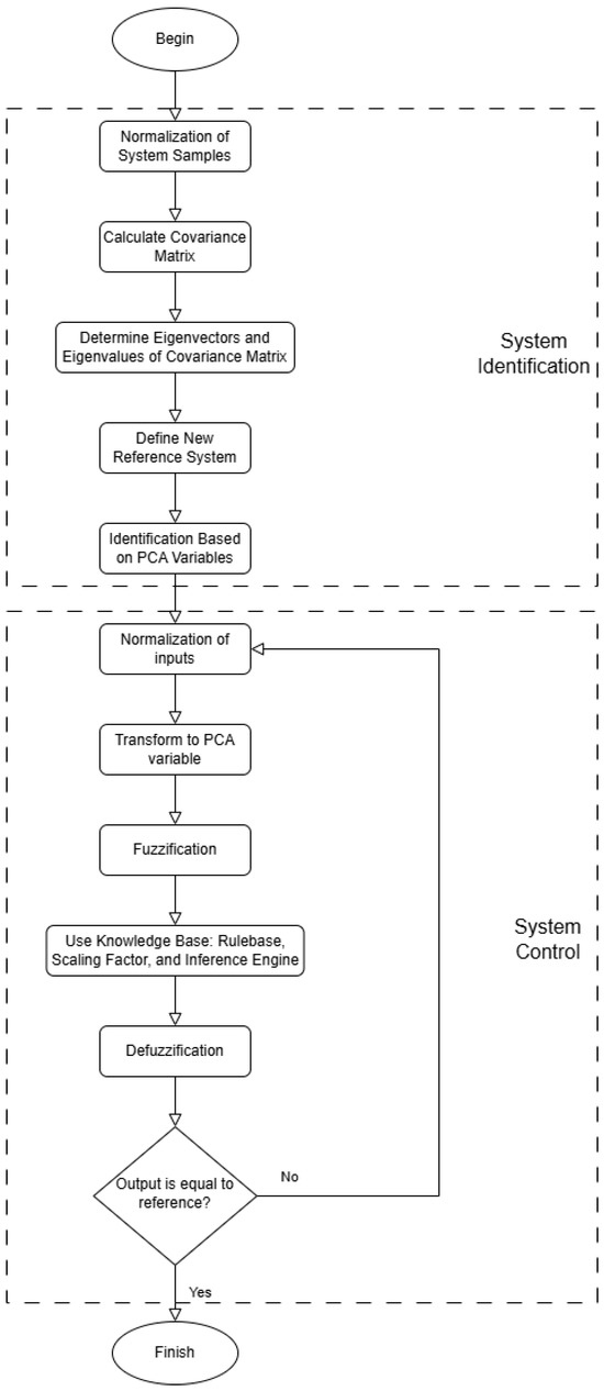
Figure 1. Flowchart of the PCA identification and control process.

3.1. Identification Using PCA

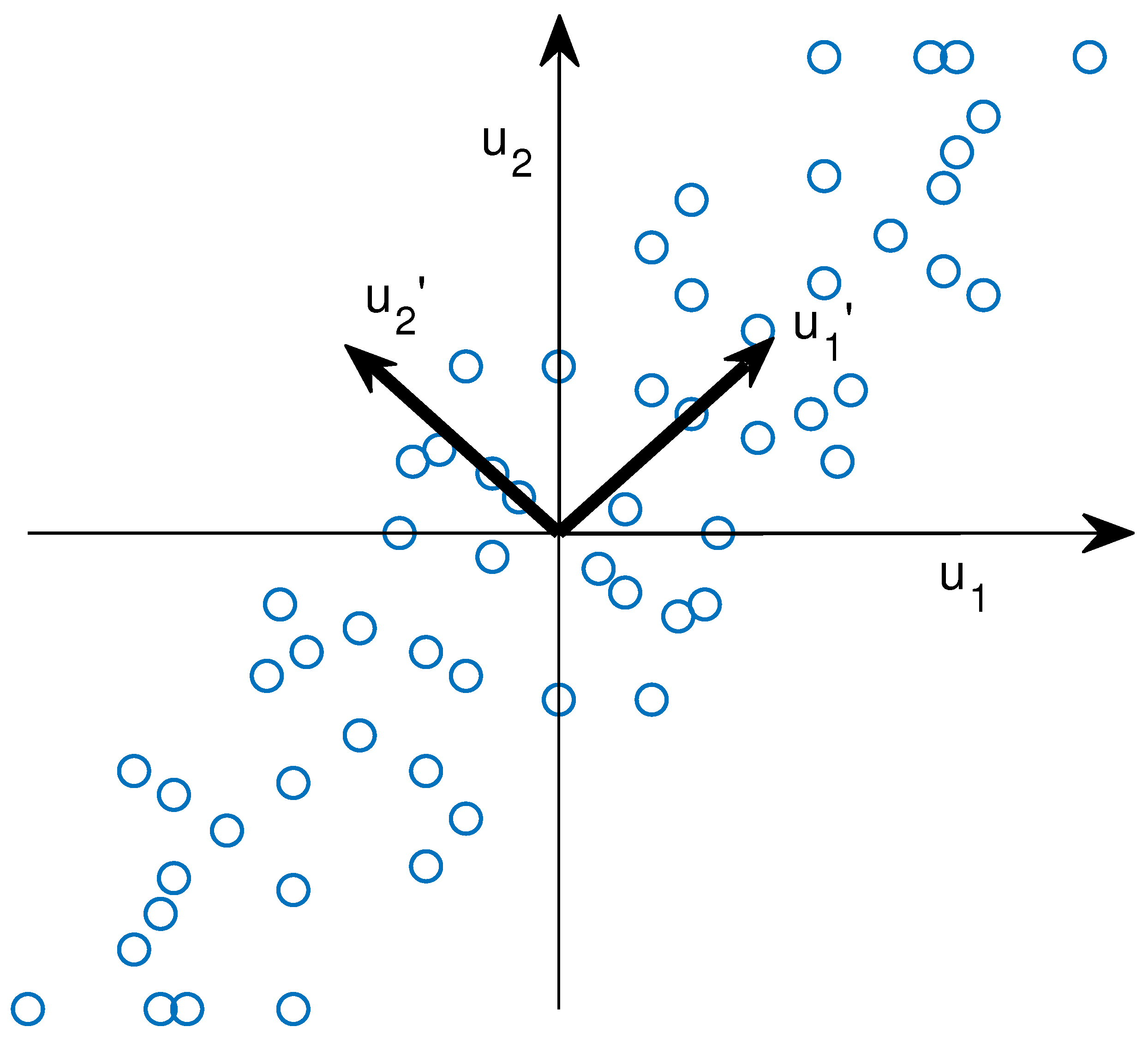
The PCA technique consists of projecting the data orthogonally onto a lower dimensional linear space, known as the principal subspace, such that the variance of the projected data are maximized (Figure 2).

Figure 2. PCA eigenvector representation.

The linear projection is defined as the one that minimizes the mean square distance between the data points and their projections.

Furthermore, the eigenvalues of the covariance matrix represent how the data are distributed, and the eigenvector of the largest eigenvalue of the covariance matrix represents the directions in which the data varies the most. Thus, the principal components are defined with the eigenvectors assigned to the largest eigenvalues of the covariance matrix.

Figure 2 shows the projection of the vectors $u_1$ and $u_2$ onto the vectors $u_1^{\prime }$ and $u_2^{\prime }$, which corresponds to the eigenvector assigned to the largest eigenvalue of the covariance matrix.

In conclusion, the signals are preprocessed to obtain the new fuzzy variables to be used in the identification of the nonlinear system. The algorithm to be followed consists of three steps:

• Normalization of samples generated for PCA-based identification.
• Calculation of the covariance matrix from the normalized samples.
• Transformation of the initial reference system to the system defined by the eigenvectors $u_1^{\prime }$ and $u_2^{\prime }$ (Figure 2).

3.1.1. Normalization

The first step is the normalization of the data, because the data processing methods are applied to the normalized data. Such a normalization starts from a set of input data. The algorithm is as follows:

$$\begin{array}{c}\hfill x_{n_i}={\displaystyle \frac{x_i-\overline{x}}{\sigma }}\end{array}$$

(8)

where the nomenclature used is

• $x_{n_i}$ is the $i^{th}$ normalized data value.
• $x_i$ is the value of the $i^{th}$ unnormalized data (initial data).
• $\overline{x}$ is the mean of k samples.
• $\sigma$ is the standard deviation of k samples.

3.1.2. Covariance Matrix

Once the data have normalized, the next step is to calculate the covariance matrix of the samples to continue the calculation of the eigenvectors and eigenvalues.

Given an n-dimensional statistical variables ($X_1$, $X_2$, $X_3$, …, $X_n$), the variance-covariance matrix will be defined as a square matrix, nxn:

$$\begin{array}{c}\hfill C=\left[\begin{array}{ccccc}{S_1}^2& S_{12}& S_{13}& \cdots & S_{1n}\\ S_{21}& {S_2}^2& S_{23}& \cdots & S_{2n}\\ S_{31}& S_{32}& {S_3}^2& \cdots & S_{2n}\\ & ⋮& & \ddots & ⋮\\ S_{n1}& S_{n2}& S_{n3}& \cdots & {S_n}^2\end{array}\right]\end{array}$$

(9)

The variances of each of the one-dimensional marginal distributions are shown in the main diagonal, and the corresponding covariances between each of the two variables $S_{ij}$ are shown in the non-diagonal elements (i, j):

$$\begin{array}{c}\hfill S_{x,y}={\displaystyle \frac{{\sum }_{i=1}^N{\sum }_{j=1}^N(x_i-\overline{x})(y_i-\overline{y})}{N}}\\ \hfill {S_x}^2={\displaystyle \frac{{\sum }_{i=1}^N(x_i-\overline{x})(x_i-\overline{x})}{N}}\end{array}$$

(10)

The value ${S_x}^2$ represents the variation of the samples on the x axis and, in the same way, ${S_y}^2$ represents the variation but on the y axis. As for the $S_{x,y}$ values, they represent the variations that occur on both axes.

3.1.3. Reference System Transformation

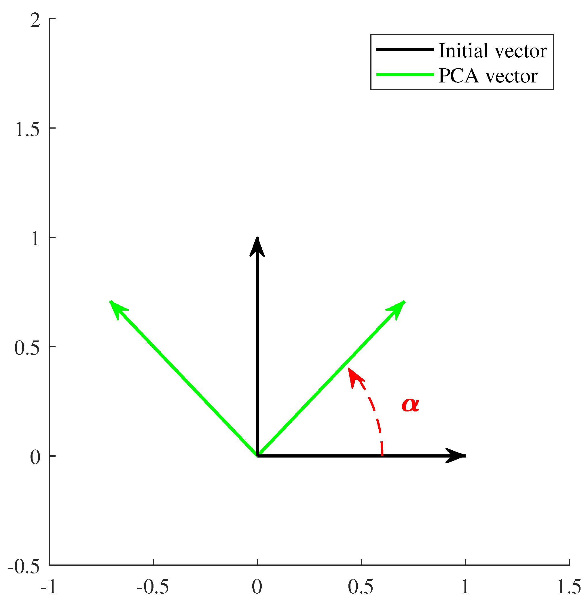
The eigenvectors of the covariance matrix are calculated, and then a transformation of the initial reference system to the one formed by the eigenvectors is performed. In fact, the procedure to be carried out involves a rotation, as illustrated in Figure 3.

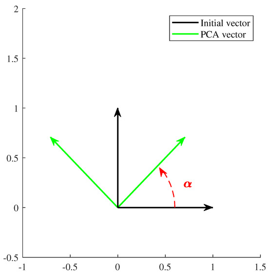
Figure 3. Rotation of the reference system.

Suppose that there is a plane belonging to ${\mathbb{R}}^2$, in which there are two reference systems named $O_{XY}$ and $O_{UV}$. Both reference systems have the origin at point O. The unit vectors of the coordinate axes of the $O_{XY}$ system are $i_x$, $j_y$, while the unit vectors of the $O_{UV}$ are $i_u$, $j_v$.

A vector belonging to the plane can be expressed in both systems:

$$\begin{array}{c}\hfill p_{xy}={[p_x,p_y]}^T=p_x{i}_x+p_y{j}_y\\ \hfill p_{uv}={[p_u,p_v]}^T=p_u{i}_u+p_v{j}_v\end{array}$$

(11)

By performing a series of transformations [25], the following matrix equivalence can be obtained:

$$\begin{array}{c}\hfill \left[\begin{array}{c}{p}_u\\ p_v\end{array}\right]=R\left[\begin{array}{c}{p}_x\\ p_y\end{array}\right]\end{array}$$

(12)

where

$$\begin{array}{c}\hfill R=\left[\begin{array}{cc}cos\alpha & sin\alpha \\ -sin\alpha & cos\alpha \end{array}\right]\end{array}$$

(13)

It is the so-called rotation matrix that serves to transform the coordinates of the $O_{XY}$ system into $O_{UV}$.

These theoretical foundations are applied to the fuzzy variable z, which has two components ($z_1$ and $z_2$), to obtain the new variable $z^{\prime }$, which is also formed with two components ($z_1^{\prime }$ and $z_2^{\prime }$) using the matrix R. The rotation matrix contains in each of its rows, the eigenvectors of the covariance matrix and, therefore, the rotation of the fuzzy variables is summarized as follows:

$$\begin{array}{c}\hfill \left[\begin{array}{c}{z}_1^{\prime }\\ z_2^{\prime }\end{array}\right]=R\left[\begin{array}{c}{z}_1\\ z_2\end{array}\right]=\left[\begin{array}{cc}{v}_{1_x}& v_{1_y}\\ v_{2_x}& v_{2_y}\end{array}\right]\left[\begin{array}{c}{z}_1\\ z_2\end{array}\right]\end{array}$$

(14)

3.2. System Control Using PCA

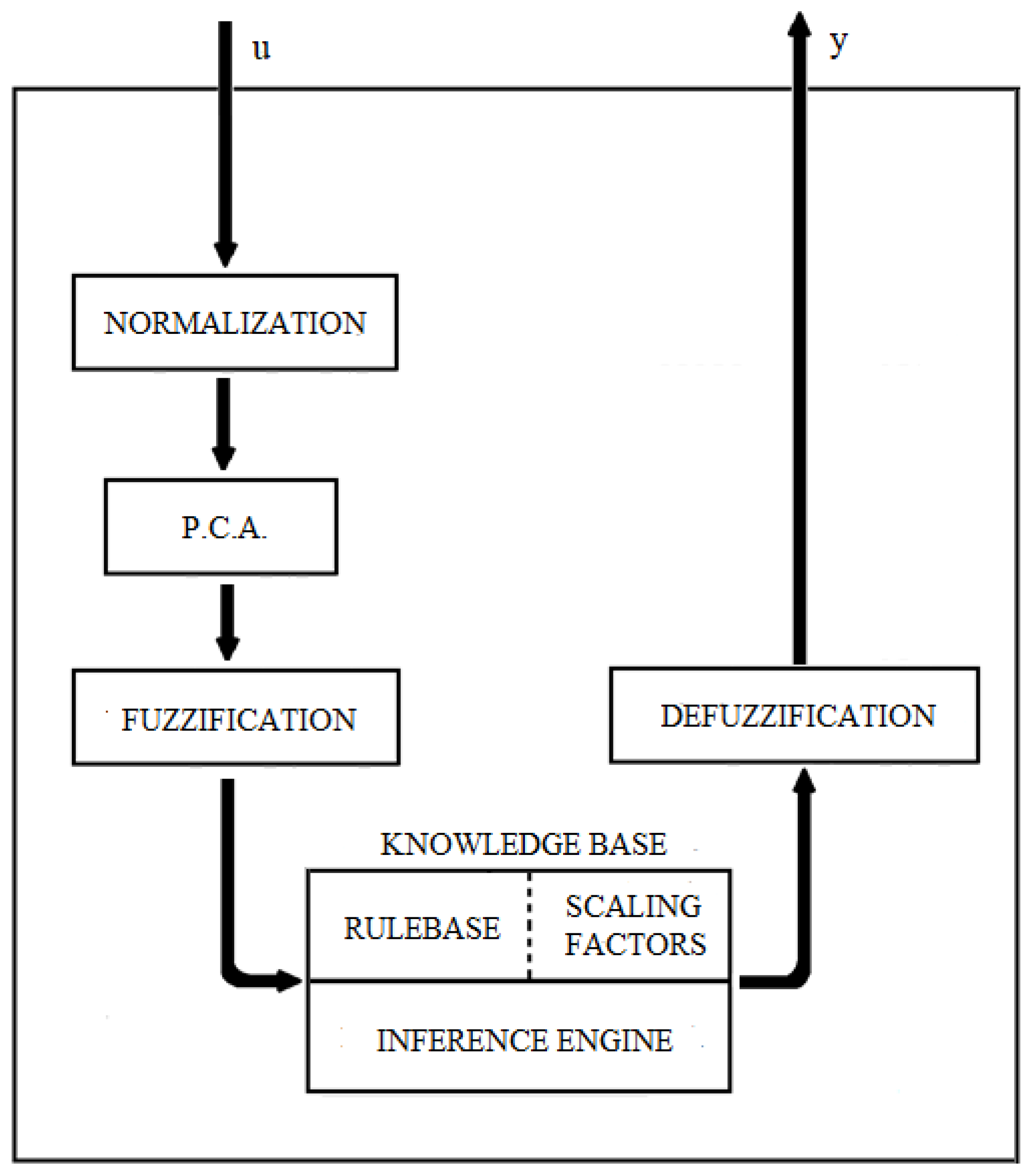
The structure used for a fuzzy control based on the PCA technique is shown in Figure 4.

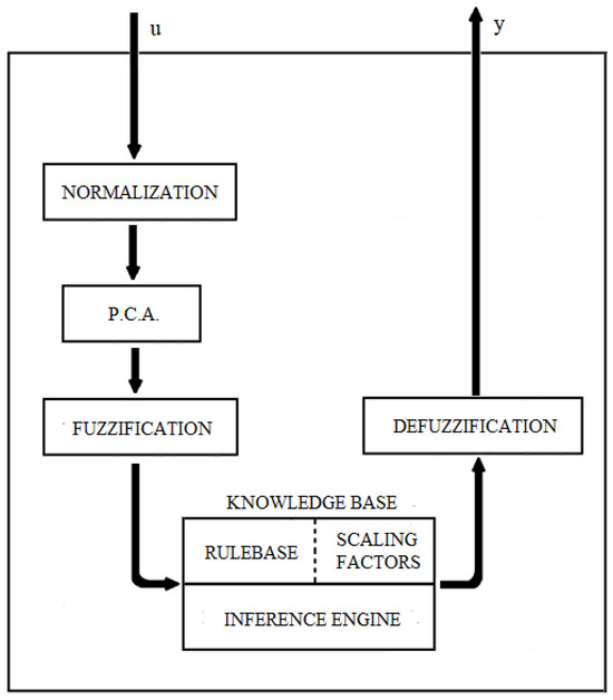
Figure 4. Basic structure of a fuzzy logic system with PCA.

The fundamental difference between the traditional T–S fuzzy control system [23] and the proposed method is that the new structure includes previous stages to normalize and perform the PCA process before fuzzification.

The PCA process transforms the fuzzy variables using the rotation matrix (R) described in Section 3.1.3. With this new fuzzy variable ($z^{\prime }$), fuzzification and defuzzification are performed.

It should be noted that no denormalization module is needed because the fuzzy control matrices and the gain matrix, called K, are obtained using non-normalized data.

4. Illustrative Example

The proposed T–S model based on PCA can be applied to any nonlinear multivariable system. In this section, the advantages of the proposed method are shown through an illustrative example of an interconnected double tank.

4.1. Interconnected Double-Tank System

The system in which the fuzzy controller based on the PCA technique will be applied is an interconnected double tank [26], shown in Figure 5.

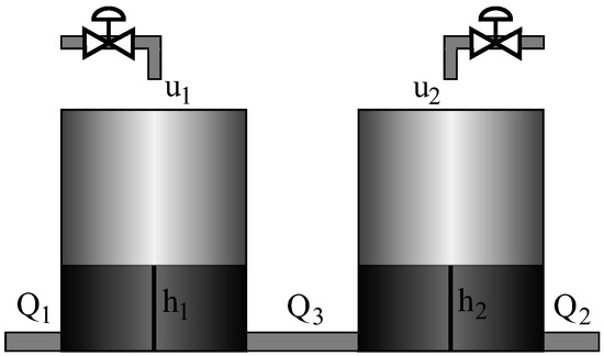
Figure 5. Interconnected double-tank system.

This system consists of two fluid tanks that are interconnected with each other by means of the pipe that transports the flow $Q_3$. It consists of two fluid inputs $u_1$ and $u_2$, which are independent in each tank. The objective of the system is to control the outflows of each tank ($Q_1$ and $Q_2$).

Considering mass balance, the dynamic equation of each tank is developed as follows:

$$\begin{array}{cc}\hfill & u_1-Q_1-Q_3=A_1{\displaystyle \frac{d{h}_1}{dt}}\hfill \\ \hfill & u_2-Q_2+Q_3=A_2{\displaystyle \frac{d{h}_2}{dt}}\hfill \end{array}$$

(15)

where $h_1$ and $h_2$ are the heights of the liquid in each tank. $A_1$ and $A_2$ are the cross-sectional areas of each tank.

On the other hand, the outflows of each tank are defined as

$$\begin{array}{c}\hfill Q_1={\alpha }_1\sqrt{2g{h}_1}\hfill \\ \hfill Q_2={\alpha }_2\sqrt{2g{h}_2}\hfill \\ \hfill Q_3=sign(h_1-h_2){\alpha }_3\sqrt{2g|h_1-h_2|}\hfill \end{array}$$

(16)

where ${\alpha }_1$, ${\alpha }_2$ and ${\alpha }_3$ are proportionality constants that depend on the coefficients of discharge and the cross-sectional area. The connection flow rate $Q_3$ is assumed positive if $h_1$ is higher than $h_2$.

The constant parameters of the double-tank system used are

$$\begin{array}{c}\hfill A_1=1 {\mathrm{m}}^2, A_2=1 {\mathrm{m}}^2\hfill \\ \hfill {\alpha }_1=0.1 {\mathrm{m}}^2, {\alpha }_2=0.1 {\mathrm{m}}^2, {\alpha }_3=0.1 {\mathrm{m}}^2\hfill \\ \hfill g=9.8 \mathrm{m}/{\mathrm{s}}^2\hfill \end{array}$$

The interconnected double-tank system can be modeled, taking the output flows $Q_1$ and $Q_2$ as state variables, with two inputs $u_1$ and $u_2$. The sampling time for the discrete model is assumed to be $T=1$ s.

The proposed discrete model for the interconnected double-tank system is as follows:

$$\begin{array}{c}\hfill \left[\begin{array}{c}{Q}_1(k+1)\\ Q_2(k+1)\end{array}\right]=\left[\begin{array}{c}{a}_{10}\\ a_{20}\end{array}\right]+\left[\begin{array}{cc}{a}_{11}& a_{12}\\ a_{21}& a_{22}\end{array}\right]\left[\begin{array}{c}{Q}_1\left(k\right)\\ Q_2\left(k\right)\end{array}\right]+\left[\begin{array}{cc}{b}_{11}& b_{12}\\ b_{21}& b_{22}\end{array}\right]\left[\begin{array}{c}{u}_1\left(k\right)\\ u_2\left(k\right)\end{array}\right]\end{array}$$

(17)

4.2. Identification of an Interconnected Double-Tank System

In this section, the system is identified in order to subsequently design the multivariable controller.

4.2.1. Nonlinear Identification Based on the Generalized T–S Model

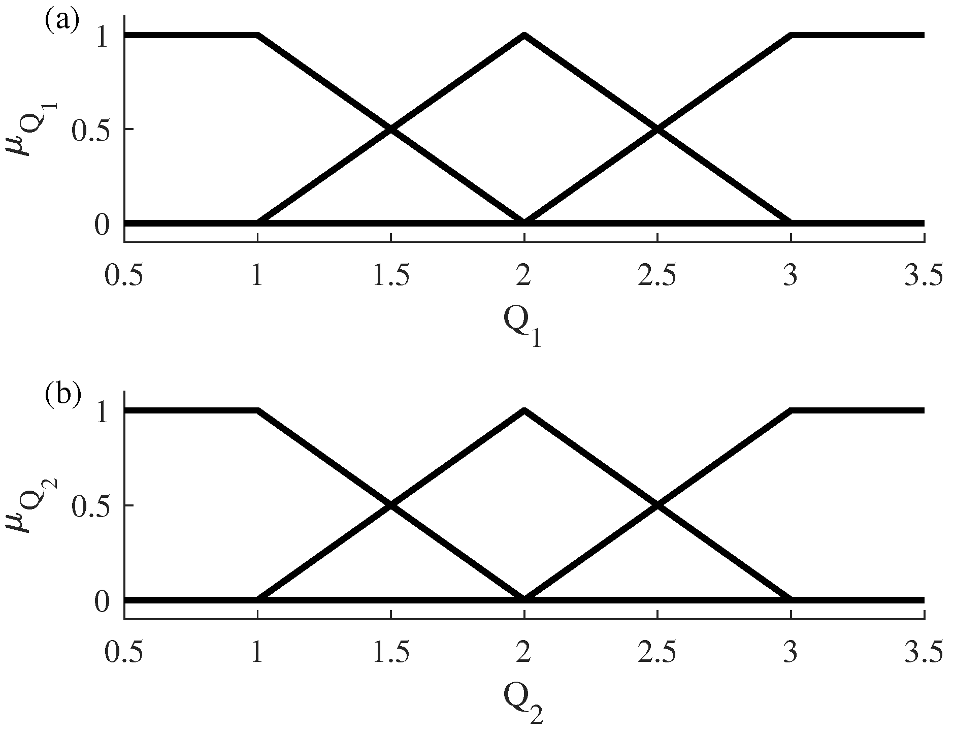
A T–S model is developed with three rules for each output variable ($Q_1$ and $Q_2$). See Figure 6.

Figure 6. Fuzzy rules using generalized T–S identification. (a) Fuzzy rules for flow $Q_1$. (b) Fuzzy rules for flow $Q_2$.

The proposed T–S model is given as follows:

$$\begin{array}{cc}\hfill S^{(i_1,i_2)}& : \mathrm{if} Q_1 \mathrm{is} M^{i_1}\mathrm{and} Q_2 \mathrm{is} M^{i_2} \mathrm{then}:\hfill \\ \hfill \left[\begin{array}{c}{Q}_1(k+1)\\ Q_2(k+1)\end{array}\right]& =\left[\begin{array}{c}{a}_{10}^{(i_1,i_2)}\\ a_{20}^{(i_1,i_2)}\end{array}\right]+\left[\begin{array}{cc}{a}_{11}^{(i_1,i_2)}& a_{12}^{(i_1,i_2)}\\ a_{21}^{(i_1,i_2)}& a_{22}^{(i_1,i_2)}\end{array}\right]\left[\begin{array}{c}{Q}_1\left(k\right)\\ Q_2\left(k\right)\end{array}\right]\hfill \\ \hfill & +\left[\begin{array}{cc}{b}_{11}^{(i_1,i_2)}& b_{12}^{(i_1,i_2)}\\ b_{21}^{(i_1,i_2)}& b_{22}^{(i_1,i_2)}\end{array}\right]\left[\begin{array}{c}{u}_1\left(k\right)\\ u_2\left(k\right)\end{array}\right]\hfill \end{array}$$

(18)

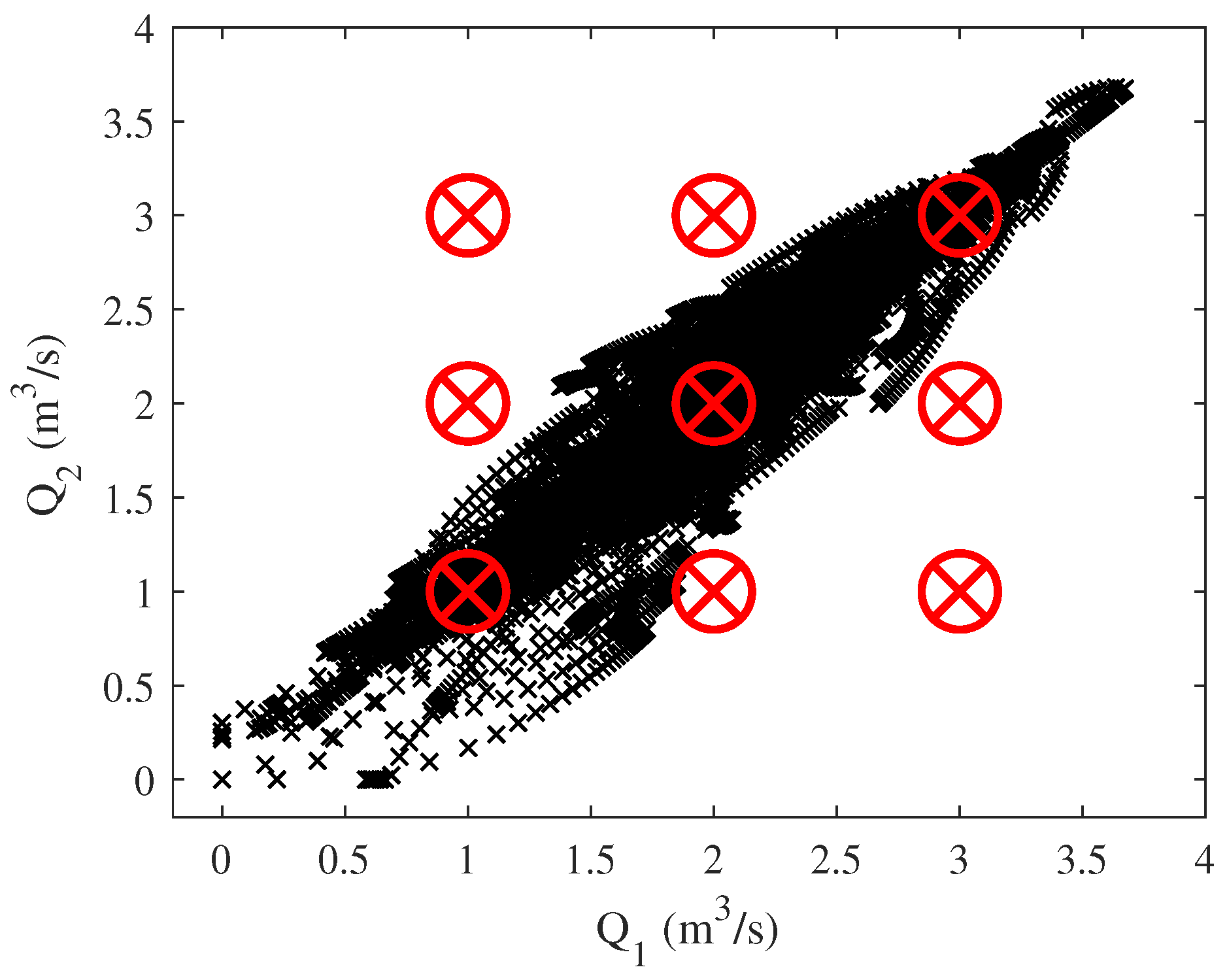
The samples used along with the distribution of the fuzzy rules are shown in Figure 7.

Figure 7. Initial samples T–S.

Firstly, the classical least squares can be used on the system data set to obtain an initial estimation, as defined in Section 2.

$$\begin{array}{cc}\hfill P_0& ={\left[\begin{array}{ccccc}{a}_{10}& a_{11}& a_{12}& b_{11}& b_{12}\\ a_{20}& a_{21}& a_{22}& b_{21}& b_{22}\end{array}\right]}^T={\left[\begin{array}{ccccc}0.00048& 0.7514& 0.2005& 0.0262& 0.0217\\ -0.0049& 0.2008& 0.7517& 0.0216& 0.0261\end{array}\right]}^T\hfill \end{array}$$

(19)

Then, the T–S fuzzy model with weighting factor $\gamma =0.0001$ [24] is

$$\begin{array}{cc}\hfill S^{(1,1)}& : \mathrm{if} Q_1 \mathrm{is} M_1^1 \mathrm{and} Q_2 \mathrm{is} M_2^1 \mathrm{then}:\hfill \\ \hfill \left[\begin{array}{c}{Q}_1(k+1)\\ Q_2(k+1)\end{array}\right]& =\left[\begin{array}{c}0.0173\\ 0.0088\end{array}\right]+\left[\begin{array}{cc}0.7914& 0.0642\\ 0.0398& 0.8396\end{array}\right]\left[\begin{array}{c}{Q}_1\left(k\right)\\ Q_2\left(k\right)\end{array}\right]\hfill \\ \hfill & +\left[\begin{array}{cc}0.0887& 0.0334\\ 0.0310& 0.0780\end{array}\right]\left[\begin{array}{c}{u}_1\left(k\right)\\ u_2\left(k\right)\end{array}\right]\hfill \\ \hfill & ⋮\hfill \end{array}$$

(20)

4.2.2. T–S Identification Based on PCA

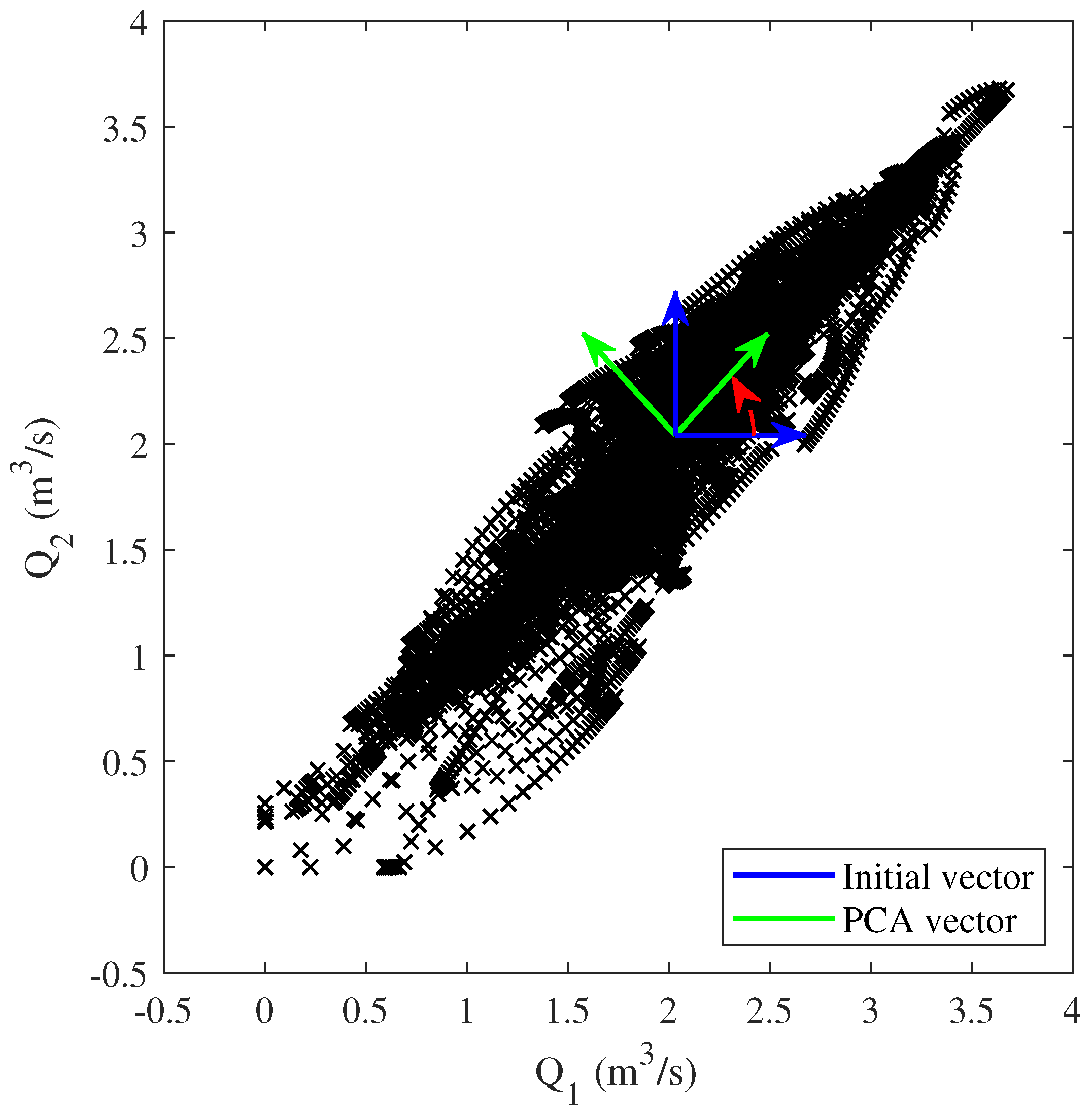
In the samples used for identification, it is shown that most of them are concentrated in a specific area of the two flows (Figure 7). Therefore, if the reference system is modified using the one formed by the PCA vectors in Figure 8, the identification process will be more accurate.

Figure 8. PCA reference system.

In this work, the mean value (Equation (21)) of the first tank flow ($Q_1$) and the mean of the second tank flow ($Q_2$) are 2.0304 m³/s and 2.0418 m³/s, respectively. The standard deviation of $Q_1$ is 0.6463 and that of $Q_2$ is 0.6794.

$$\begin{array}{c}\hfill \overline{Q_i}={\displaystyle \frac{{\sum }_{k=1}^N{Q}_i\left(k\right)}{N}}\end{array}$$

(21)

In the interconnected double-tank system, there are two one-dimensional distributions: the first is the flow of the first tank ($Q_1$) and the other is of the second tank ($Q_2$). Therefore, the covariances of the normalized samples are as follows:

$$\begin{array}{cc}\hfill {S_{Q_{n_1}}}^2& =1\hfill \\ \hfill S_{Q_{n_1},Q_{n_2}}& =0.946\hfill \\ \hfill S_{Q_{n_2},Q_{n_1}}& =0.946\hfill \\ \hfill {S_{Q_{n_2}}}^2& =1\hfill \end{array}$$

(22)

The covariance matrix of dimension $2\times 2$ with the calculated covariances is

$$\begin{array}{c}\hfill C=\left[\begin{array}{cc}{S_{Q_{n_1}}}^2& S_{Q_{n_1},Q_{n_2}}\\ S_{Q_{n_2},Q_{n_1}}& {S_{Q_{n_2}}}^2\end{array}\right]=\left[\begin{array}{cc}1& 0.946\\ 0.946& 1\end{array}\right]\end{array}$$

(23)

To continue with the algorithm, the eigenvectors and eigenvalues of the covariance matrix are calculated as follows:

$$\begin{array}{cc}\hfill & |C-\lambda I|=0\hfill \\ \hfill & \left|\left[\begin{array}{cc}1& 0.946\\ 0.946& 1\end{array}\right]-\left[\begin{array}{cc}\lambda & 0\\ 0& \lambda \end{array}\right]\right|=0\hfill \\ \hfill & {\lambda }_1=1.946{\lambda }_2=0.054\hfill \end{array}$$

(24)

When the eigenvalues have been obtained, the eigenvector assigned to each eigenvalue is calculated by the following equation:

$$\begin{array}{cc}\hfill & (C-{\lambda }_{1}I)v_1=\theta \hfill \\ \hfill & (C-{\lambda }_{2}I)v_2=\theta \hfill \\ \hfill v_1=& \left[\begin{array}{cc}-0.7071& 0.7071\end{array}\right]\hfill \\ \hfill v_2=& \left[\begin{array}{cc}0.7071& 0.7071\end{array}\right]\hfill \end{array}$$

(25)

The samples obtained from the new fuzzy variables ($z_1$ and $z_2$) are shown in Figure 9, after the normalization process, vector calculation of the new reference system (eigenvectors of the covariance matrix) and the rotation to the new reference system have been performed.

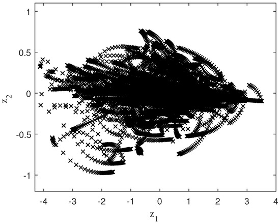
Figure 9. Initial samples applying PCA.

Next, an identification is performed by defining new rules for the fuzzy variable $z_1$ only. This method will be referred to as PCA 1D.

Finally, the system is identified by defining new fuzzy rules using the two dimensions ($z_1$ and $z_2$) obtained in the PCA process. This method is called PCA 2D.

4.2.3. PCA 1D Technique

In this section, the T–S model is developed using five fuzzy rules fitted by the PCA 1D technique; therefore, the new fuzzy variable $z_1$ will be used.

The proposed T–S model using the PCA 1D technique is given as follows:

$$\begin{array}{cc}\hfill & S^{\left(i\right)}: \mathrm{if} z_1 \mathrm{is} M^{i_1} \mathrm{then}:\hfill \\ \hfill \left[\begin{array}{c}{Q}_1(k+1)\\ Q_2(k+1)\end{array}\right]& =\left[\begin{array}{c}{a}_{10}^{\left(i\right)}\\ a_{20}^{\left(i\right)}\end{array}\right]+\left[\begin{array}{cc}{a}_{11}^{\left(i\right)}& a_{12}^{\left(i\right)}\\ a_{21}^{\left(i\right)}& a_{22}^{\left(i\right)}\end{array}\right]\left[\begin{array}{c}{Q}_1\left(k\right)\\ Q_2\left(k\right)\end{array}\right]\hfill \\ \hfill & +\left[\begin{array}{cc}{b}_{11}^{\left(i\right)}& b_{12}^{\left(i\right)}\\ b_{21}^{\left(i\right)}& b_{22}^{\left(i\right)}\end{array}\right]\left[\begin{array}{c}{u}_1\left(k\right)\\ u_2\left(k\right)\end{array}\right]\hfill \end{array}$$

(26)

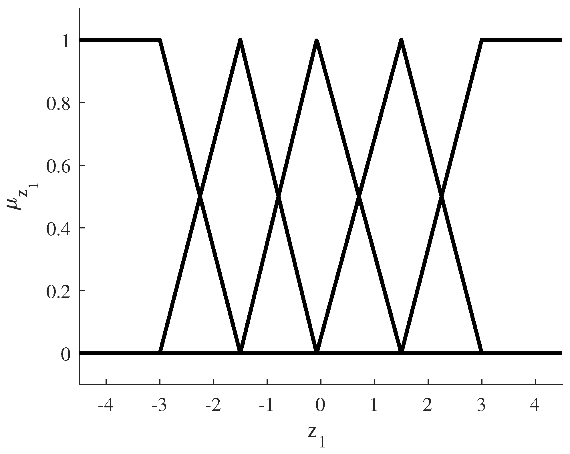
The placement of fuzzy rules is determined by analyzing the histogram of the variable $z_1$ (Figure 10). The rules are distributed to cover the widest possible range of samples. Thus, the triangular shaped rules will reach a weight of 1 at specific values: −3, −1.5, 0, 1.5, and 3. This approach optimizes the coverage of the rules in the sample space, improving the performance of the system.

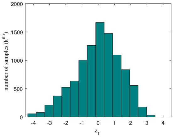
Figure 10. Histogram of the variable $z_1$.

The five triangular-shaped membership functions used can be seen in Figure 11. They are defined in the new fuzzy variable $z_1$.

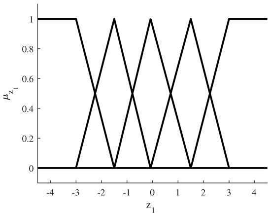
Figure 11. Fuzzy rules using PCA 1D identification.

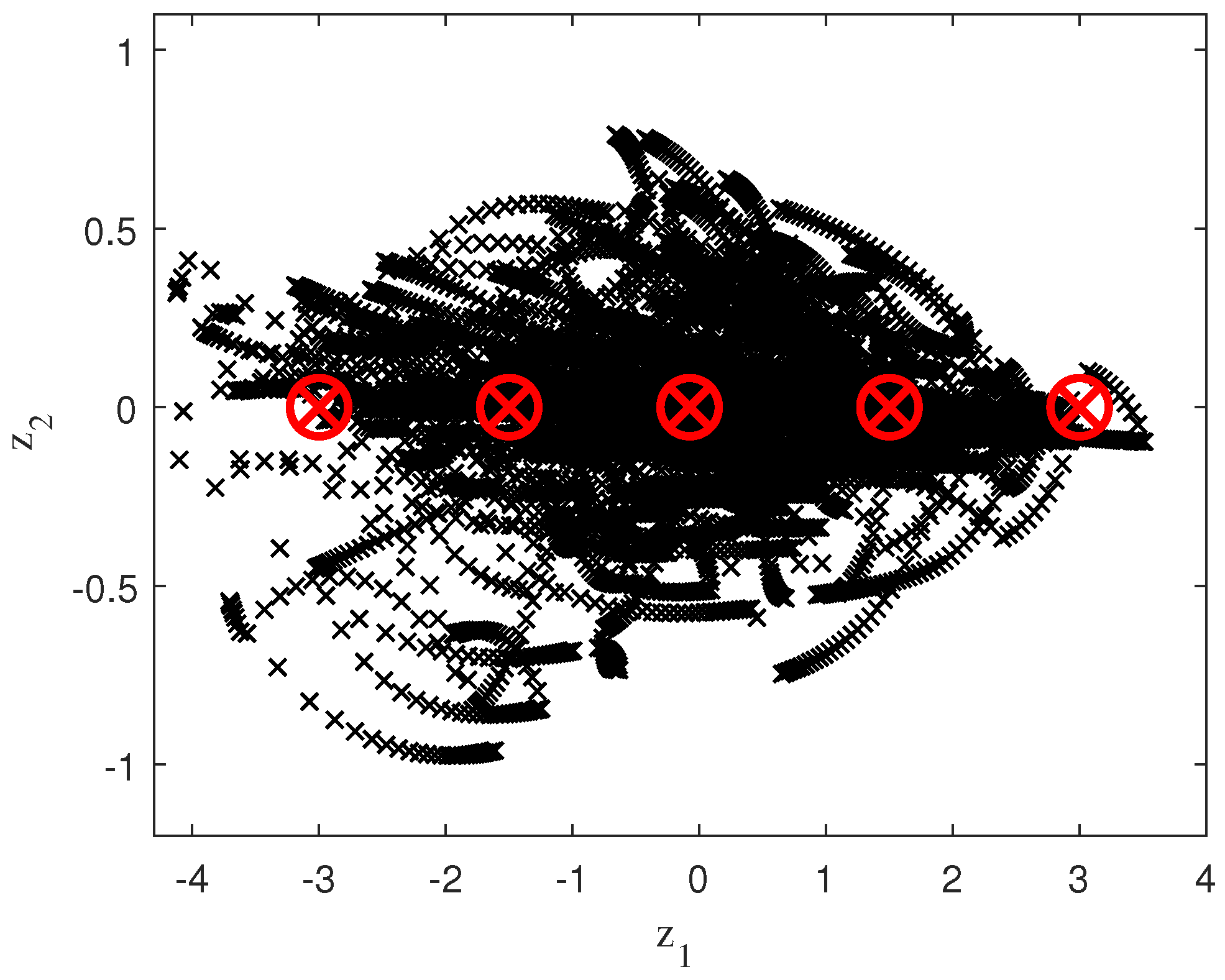
The samples used for identification along with the distribution of the five fuzzy rules are reflected in Figure 12, once the PCA process has been applied.

Figure 12. Initial samples and fuzzy rules with PCA 1D.

By applying the inverse process of the PCA technique, the position of the fuzzy rules is calculated and shown in Figure 13, verifying that the rules are located in the area of higher concentration of samples fitting perfectly to the nonlinear system used.

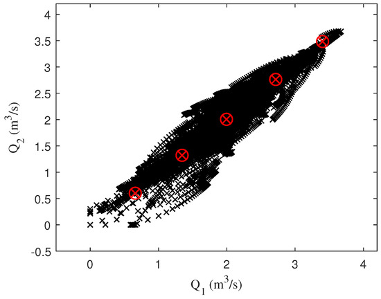
Figure 13. Flows diagram $Q_1$–$Q_2$ using PCA 1D fuzzy rules.

Finally, the T–S fuzzy model using the PCA 1D technique and $\gamma =0.0001$ becomes

$$\begin{array}{cc}\hfill & S^{\left(1\right)}: \mathrm{if} z_1 \mathrm{is} M_1 \mathrm{then}:\hfill \\ \hfill \left[\begin{array}{c}{Q}_1(k+1)\\ Q_2(k+1)\end{array}\right]& =\left[\begin{array}{c}0.0251\\ 0.0241\end{array}\right]+\left[\begin{array}{cc}0.7442& 0.0564\\ 0.0172& 0.7953\end{array}\right]\left[\begin{array}{c}{Q}_1\left(k\right)\\ Q_2\left(k\right)\end{array}\right]\hfill \\ \hfill & +\left[\begin{array}{cc}0.1103& 0.0454\\ 0.0403& 0.0940\end{array}\right]\left[\begin{array}{c}{u}_1\left(k\right)\\ u_2\left(k\right)\end{array}\right]\hfill \\ \hfill & ⋮\hfill \end{array}$$

(27)

4.2.4. PCA 2D Technique

In this section, a T–S model is developed using the two dimensions provided by the PCA technique ($z_1$ and $z_2$), so that the rules will be adjusted to the area where the samples are more concentrated and the identification will be more accurate. The total number of rules used is nine, establishing three rules for each variable.

The proposed T–S model using the two variables provided by the PCA technique is summarized as follows:

$$\begin{array}{cc}\hfill & S^{(i_1,i_2)}: \mathrm{if} z_1 \mathrm{is} M^{i_1} \mathrm{and} z_2 \mathrm{is} M^{i_2} \mathrm{then}:\hfill \\ \hfill \left[\begin{array}{c}{Q}_1(k+1)\\ Q_2(k+1)\end{array}\right]& =\left[\begin{array}{c}{a}_{10}^{(i_1,i_2)}\\ a_{20}^{(i_1,i_2)}\end{array}\right]+\left[\begin{array}{cc}{a}_{11}^{(i_1,i_2)}& a_{12}^{(i_1,i_2)}\\ a_{21}^{(i_1,i_2)}& a_{22}^{(i_1,i_2)}\end{array}\right]\left[\begin{array}{c}{Q}_1\left(k\right)\\ Q_2\left(k\right)\end{array}\right]\hfill \\ \hfill & +\left[\begin{array}{cc}{b}_{11}^{(i_1,i_2)}& b_{12}^{(i_1,i_2)}\\ b_{21}^{(i_1,i_2)}& b_{22}^{(i_1,i_2)}\end{array}\right]\left[\begin{array}{c}{u}_1\left(k\right)\\ u_2\left(k\right)\end{array}\right]\hfill \end{array}$$

(28)

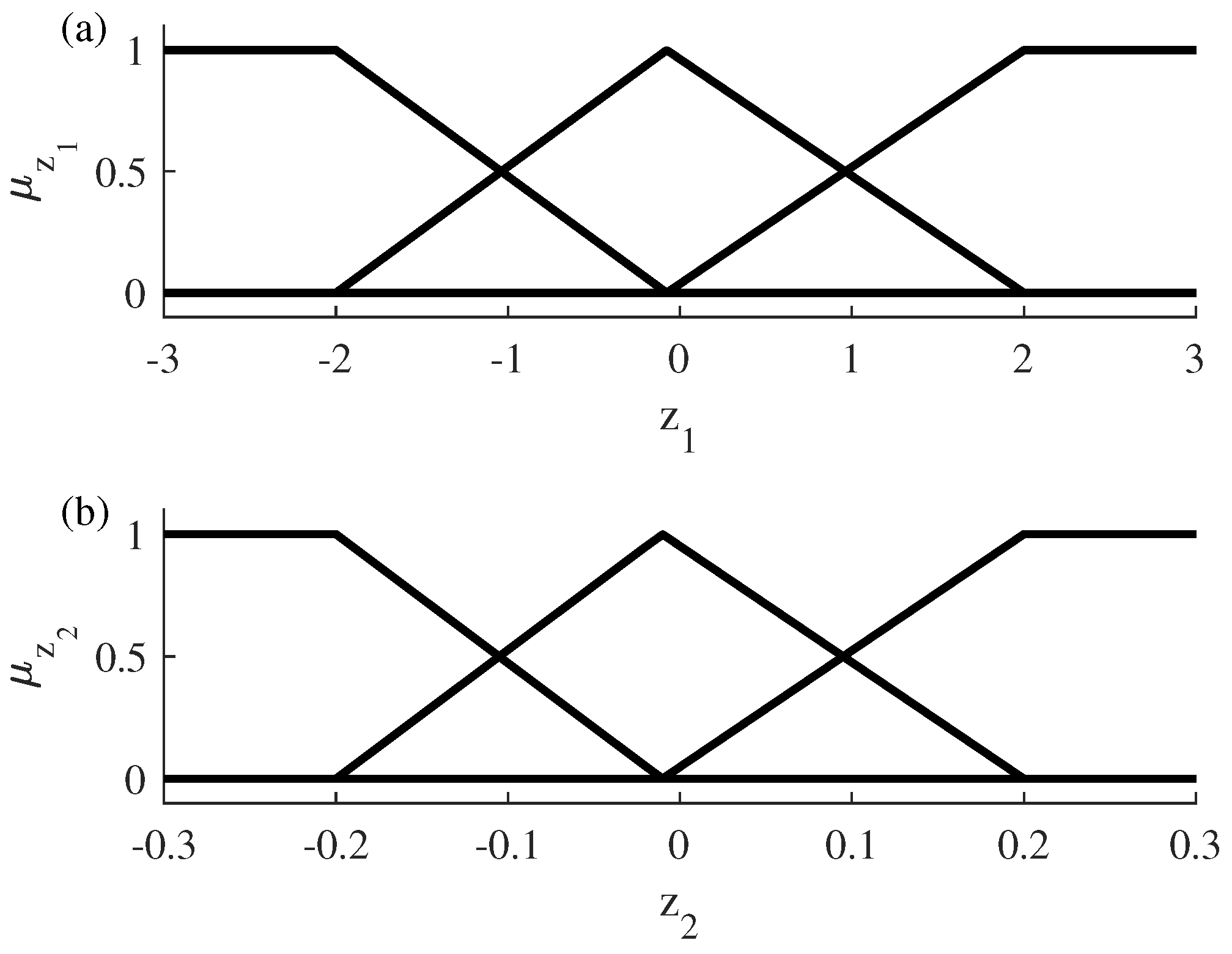
Following the methodology used in the PCA 1D identification, the histogram of the variables $z_1$ and $z_2$ is examined (Figure 14). Triangular rules reach a maximum weight of 1 at specific values—in $z_1$, −2, 0, 2; in $z_2$, −0.2, 0, 0.2—to cover the largest possible area within the region of highest data concentration.

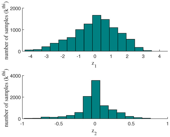
Figure 14. Histogram of variables $z_1$ and $z_2$.

The three membership functions of each fuzzy variable are shown in Figure 15.

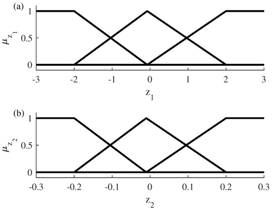
Figure 15. Fuzzy rules using PCA 2D identification. (a) Fuzzy rules for the variable $z_1$. (b) Fuzzy rules for the variable $z_2$.

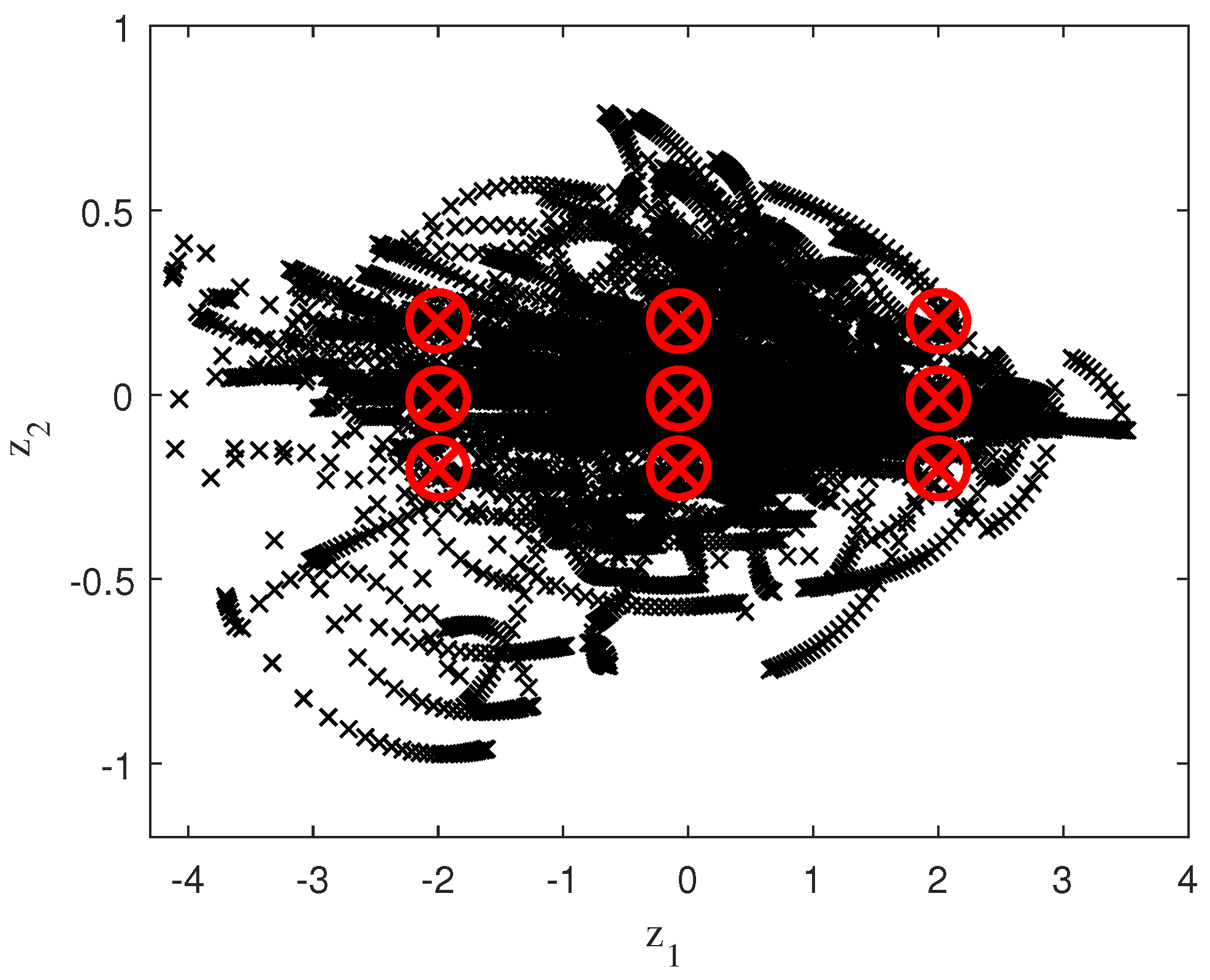
The samples used for identification together with the distribution of the nine fuzzy rules, once the PCA 2D process (normalization and rotation to the new reference system) has been applied, is shown in Figure 16.

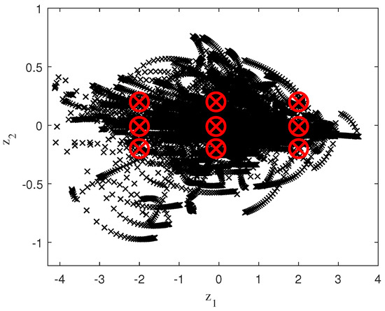
Figure 16. Initial samples applying PCA 2D technique and their respective fuzzy rules.

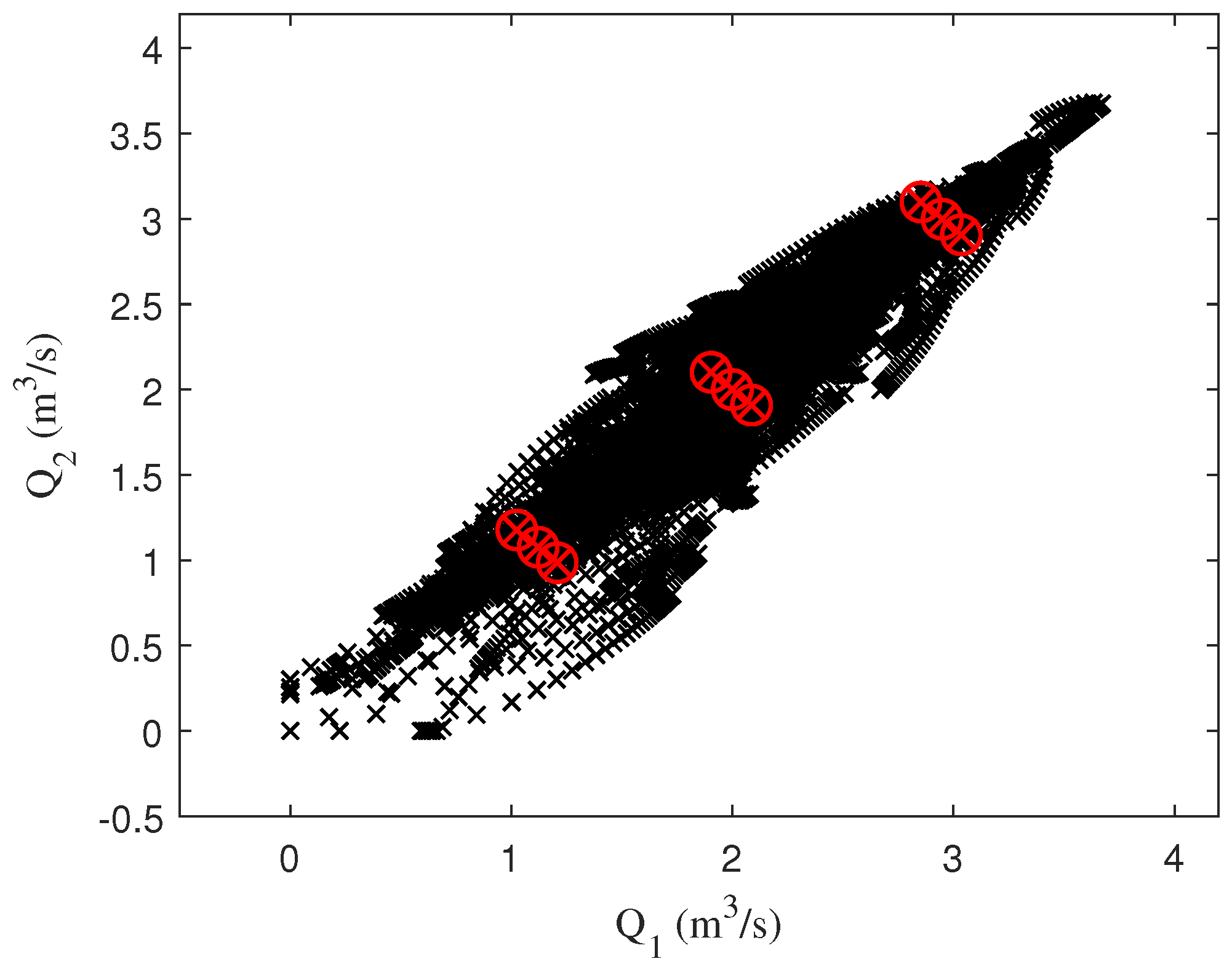
The location of fuzzy rules is calculated by using the inverse process of the PCA technique, as shown in Figure 17, where it can be observed that they are positioned in the area where most of the samples are concentrated.

Figure 17. Flow diagram $Q_1$ – $Q_2$ using PCA 2D fuzzy rules.

Finally, the T–S fuzzy model using the PCA 2D technique and $\gamma =0.0001$ is

$$\begin{array}{cc}\hfill & S^{(1,1)}: \mathrm{if} z_1 \mathrm{is} M_1^1 \mathrm{and} z_2 \mathrm{is} M_2^1 \mathrm{then}:\hfill \\ \hfill \left[\begin{array}{c}{Q}_1(k+1)\\ Q_2(k+1)\end{array}\right]& =\left[\begin{array}{c}-0.0050\\ -0.0151\end{array}\right]+\left[\begin{array}{cc}0.8482& 0.0405\\ 0.1270& 0.8032\end{array}\right]\left[\begin{array}{c}{Q}_1\left(k\right)\\ Q_2\left(k\right)\end{array}\right]\hfill \\ \hfill & +\left[\begin{array}{cc}0.0752& 0.0098\\ 0.0103& 0.1033\end{array}\right]\left[\begin{array}{c}{u}_1\left(k\right)\\ u_2\left(k\right)\end{array}\right]\hfill \\ \hfill & ⋮\hfill \end{array}$$

(29)

4.2.5. Comparison of Identification Methods

The results obtained in the identification of the system with the three proposed methods (generalized T–S without applying PCA, T–S based on the PCA 1D technique and T–S based on the PCA 2D technique) are summarized below, where the root mean squared error (RMSE) was calculated for each one of the three methods. The results obtained are summarized in Table 1.

Table 1. Errors made in the identification of the nonlinear system.

Identification Type	Number of Rules	% Error RMSE in ${\mathit{Q}}_1$	% Error RMSE in ${\mathit{Q}}_2$	Mean of % Error RMSE
Generalized T–S	9	0.419	0.396	0.408
T–S PCA 1D	5	0.418	0.411	0.415
T–S PCA 2D	9	0.365	0.334	0.349

The main advantage of the PCA technique appears with the use of PCA 1D identification, where the number of rules is reduced by almost half and the error remains around 0.4, similar to that of the generalized T–S identification without using PCA. This represents a very high computational cost saving.

With respect to PCA 2D, the number of rules is the same as that used with the T–S identification without using PCA. The advantage is that the error is reduced compared to that made with T–S identification without using PCA and T–S identification based on PCA 1D.

5. Control of an Interconnected Tank System Applying the Proposed PCA Method

In this section, an incremental model control approach is presented to control the nonlinear system of interconnected tanks. In this approach, three models will be implemented: generalized T–S, PCA 1D and PCA 2D. Finally, the results obtained will be shown to demonstrate the effectiveness of each of the methodologies used.

5.1. Optimal Control Based on T–S Model, Incremental Approach and PCA Proposed Method

Three models are proposed, a generalized T–S, PCA 1D and PCA 2D based on the incremental model [10], which has the great advantage of zero steady state error due to its control action, which is equivalent to introducing an integral action.

5.1.1. Optimal and Incremental Control Based on Generalized T–S Model

A fuzzy model is presented based on the optimal control with an incremental state model [10] and using the three fuzzy rules presented in Section 4.2.1 (see Figure 6). The control action is obtained according to the following equation:

$$\begin{array}{cc}\hfill S^{\left(i_1\right)}: \mathrm{if} Q_1\left(k\right) \mathrm{is} M_1^{i_1}& \mathrm{and} Q_2\left(k\right)\mathrm{is} M_2^{i_1} \mathrm{then}:\hfill \\ \hfill \Delta u{\left(k\right)}_{\left(i_1\right)}=& K_{LQ{R}_{inc}}^{\left(i_1\right)}(x_r-x_a)\hfill \\ \hfill u{\left(k\right)}_{\left(i_1\right)}=& u(k-1)+\Delta u{\left(k\right)}_{\left(i_1\right)}\hfill \\ \hfill & ⋮\hfill \end{array}$$

(30)

where

$$x_r=\left[\begin{array}{c}{y}_r\left(k\right)\\ 0\end{array}\right]x_a=\left[\begin{array}{c}y\left(k\right)\\ \Delta x\left(k\right)\end{array}\right]$$

Firstly, due to the use of the incremental model, the extended system matrices $A_a$, $B_a$ and $C_a$ [10] are defined for each fuzzy rule based on the matrices A, B and C from the discrete model:

$$A_a=\left[\begin{array}{cc}I& CA\\ 0& A\end{array}\right]B_a=\left[\begin{array}{c}CB\\ B\end{array}\right]C_a=\left[\begin{array}{cc}I& 0\end{array}\right]$$

Applying to the double-tank system:

$$\begin{array}{cc}\hfill S^{(1,1)}: \mathrm{if} Q_1\left(k\right) \mathrm{is} M_1^1& \mathrm{and} Q_2\left(k\right) \mathrm{is} M_2^1 \mathrm{then}:\hfill \\ \hfill A_a^{(1,1)}=\left[\begin{array}{cccc}1& 0& 0.7914& 0.0642\\ 0& 1& 0.0398& 0.8396\\ 0& 0& 0.7914& 0.0642\\ 0& 0& 0.0398& 0.8396\end{array}\right]& B_a^{(1,1)}=\left[\begin{array}{cc}0.0887& 0.0334\\ 0.0310& 0.0780\\ 0.0887& 0.0334\\ 0.0310& 0.0780\end{array}\right]\hfill \\ \hfill C_a^{(1,1)}=& \left[\begin{array}{cccc}1& 0& 0& 0\\ 0& 1& 0& 0\end{array}\right]\hfill \\ \hfill & ⋮\hfill \end{array}$$

(31)

Secondly, the following Q and R matrices are used for this controller model:

$$Q_{inc}=\left[\begin{array}{cccc}1& 0& 0& 0\\ 0& 1& 0& 0\\ 0& 0& 1& 0\\ 0& 0& 0& 1\end{array}\right]R_{inc}=\left[\begin{array}{cc}1& 0\\ 0& 1\end{array}\right]$$

The diagonal structure of the Q matrix with unit weights emphasizes equal importance to all state variables in the system, ensuring a balanced evaluation of state performance. On the other hand, the identity structure of the R matrix ensures that the control effort is equally penalized across all input channels, maintaining a trade-off between state performance and energy consumption. This choice of Q and R matrices provides a robust and balanced framework for the controller design.

The state controller matrix based on the incremental using the LQR-controller-based discrete state model is

$$\begin{array}{cc}\hfill & S^{(1,1)}: \mathrm{if} Q_1\left(k\right) \mathrm{is} M_1^1 \mathrm{and} Q_2\left(k\right) \mathrm{is} M_2^1 \mathrm{then}:\hfill \\ \hfill & K_{LQ{R}_{inc}}^{(1,1)}=\left[\begin{array}{cccc}0.8697& -0.0458& 2.1787& 0.0871\\ -0.0506& 0.8706& 0.0052& 2.6218\end{array}\right]\hfill \\ \hfill & ⋮\hfill \end{array}$$

5.1.2. Optimal and Incremental Control Based on T–S Model Using PCA 1D

In this section, an approach based on the PCA technique is proposed with the objective of obtaining tracking results similar to the T–S control model, with the exemption of reducing the fuzzy rules from nine to five.

The control method based on the incremental model using the PCA 1D technique and the five fuzzy rules presented in Section 4.2.3 (see Figure 11) obtains the control action according to the following equation:

$$\begin{array}{cc}\hfill S^{\left(i_1\right)}: \mathrm{if}& z_1 \left(k\right) \mathrm{is} M_1^{i_1} \mathrm{then}:\hfill \\ \hfill \Delta u{\left(k\right)}_{\left(i_1\right)}=& K_{LQ{R}_{PCA1Dinc}}^{\left(i_1\right)}(x_r-x_a)\hfill \\ \hfill u{\left(k\right)}_{\left(i_1\right)}=& u(k-1)+\Delta u{\left(k\right)}_{\left(i_1\right)}\hfill \\ \hfill & ⋮\hfill \end{array}$$

(32)

Then, the extended matrices ($A_a$, $B_a$ and $C_a$) are obtained for each of the rules to calculate the gain matrix:

$$\begin{array}{cc}\hfill S^{\left(1\right)}: \mathrm{if}& z_1\left(k\right) \mathrm{is} M_1^1 \mathrm{then}:\hfill \\ \hfill A_a^{\left(1\right)}=\left[\begin{array}{cccc}1& 0& 0.7442& 0.0564\\ 0& 1& 0.0172& 0.7953\\ 0& 0& 0.7442& 0.0564\\ 0& 0& 0.0172& 0.7953\end{array}\right]& B_a^{\left(1\right)}=\left[\begin{array}{cc}0.1103& 0.0454\\ 0.0403& 0.0940\\ 0.1103& 0.0454\\ 0.0403& 0.0940\end{array}\right]\hfill \\ \hfill C_a^{\left(1\right)}=& \left[\begin{array}{cccc}1& 0& 0& 0\\ 0& 1& 0& 0\end{array}\right]\hfill \end{array}$$

(33)

Finally, the state controller matrix based on the PCA 1D model and using the same weighting matrices defined in Section 5.1.1 is

$$\begin{array}{cc}\hfill & S^{(1,1)}: \mathrm{if} Q_1\left(k\right) \mathrm{is} M_1^1 \mathrm{and} Q_2\left(k\right) \mathrm{is} M_2^1 \mathrm{then}:\hfill \\ \hfill & K_{LQ{R}_{PCA1Dinc}}^{(1,1)}=\left[\begin{array}{cccc}0.8595& -0.0698& 1.7893& -0.0491\\ -0.0316& 0.8669& -0.1055& 2.1607\end{array}\right]\hfill \\ \hfill & ⋮\hfill \end{array}$$

5.1.3. Optimal and Incremental Control Based on T–S Model Using PCA 2D

In this section, a control model that uses the PCA 2D technique is presented; moreover, the incremental model is added using the three fuzzy rules in each variable presented in Section 4.2.4 (see Figure 15). The control action is obtained according to the following equation:

$$\begin{array}{cc}\hfill S^{\left(i_1\right)}: \mathrm{if}& z_1\left(k\right) \mathrm{is} M_1^{i_1} \mathrm{and} z_2\left(k\right)\mathrm{is} M_2^{i_1} \mathrm{then}:\hfill \\ \hfill \Delta u{\left(k\right)}_{\left(i_1\right)}=& K_{LQ{R}_{PCA2Dinc}}^{\left(i_1\right)}(x_r-x_a)\hfill \\ \hfill u{\left(k\right)}_{\left(i_1\right)}=& u(k-1)+\Delta u{\left(k\right)}_{\left(i_1\right)}\hfill \\ \hfill & ⋮\hfill \end{array}$$

(34)

Firstly, the extended matrices ($A_a$, $B_a$ and $C_a$) of each of the rules are obtained to calculate the gain matrix:

$$\begin{array}{cc}\hfill S^{(1,1)}: \mathrm{if} z_1\left(k\right) \mathrm{is} M_1^1& \mathrm{and} z_2\left(k\right)\mathrm{is} M_2^1 \mathrm{then}:\hfill \\ \hfill A_a^{(1,1)}=\left[\begin{array}{cccc}1& 0& 0.8482& 0.0405\\ 0& 1& 0.1270& 0.8032\\ 0& 0& 0.8482& 0.0405\\ 0& 0& 0.1270& 0.8032\end{array}\right]& B_a^{(1,1)}=\left[\begin{array}{cc}0.0752& 0.0098\\ 0.0103& 0.1033\\ 0.0752& 0.0098\\ 0.0103& 0.1033\end{array}\right]\hfill \\ \hfill C_a^{(1,1)}=& \left[\begin{array}{cccc}1& 0& 0& 0\\ 0& 1& 0& 0\end{array}\right]\hfill \\ \hfill & ⋮\hfill \end{array}$$

(35)

Thus, the state controller matrix based on the PCA 2D model and using the same weighting matrices defined in Section 5.1.1 is

$$\begin{array}{cc}\hfill & S^{(1,1)}: \mathrm{if} Q_1\left(k\right) \mathrm{is} M_1^1 \mathrm{and} Q_2\left(k\right)\mathrm{is} M_2^1 \mathrm{then}:\hfill \\ \hfill & K_{LQ{R}_{PCA2Dinc}}^{(1,1)}=\left[\begin{array}{cccc}0.8683& -0.0014& 2.7763& 0.2959\\ -0.0596& 0.8479& 0.6255& 2.1461\end{array}\right]\hfill \\ \hfill & ⋮\hfill \end{array}$$

5.1.4. Comparison of T–S Control Models Based on Incremental Approach and PCA Technique

In this section, the results obtained with the three models (T–S without using PCA, PCA 1D and PCA 2D) are discussed.

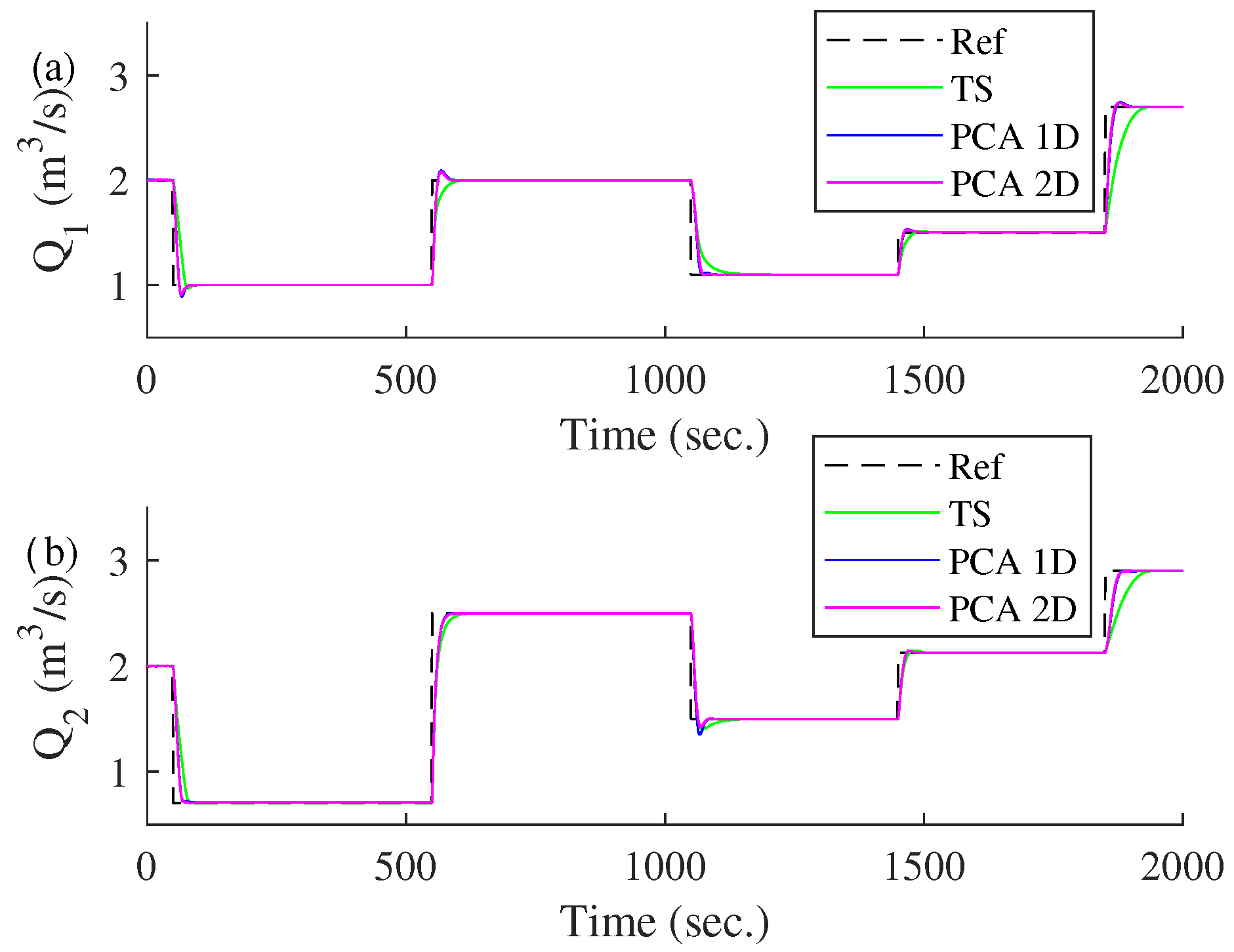
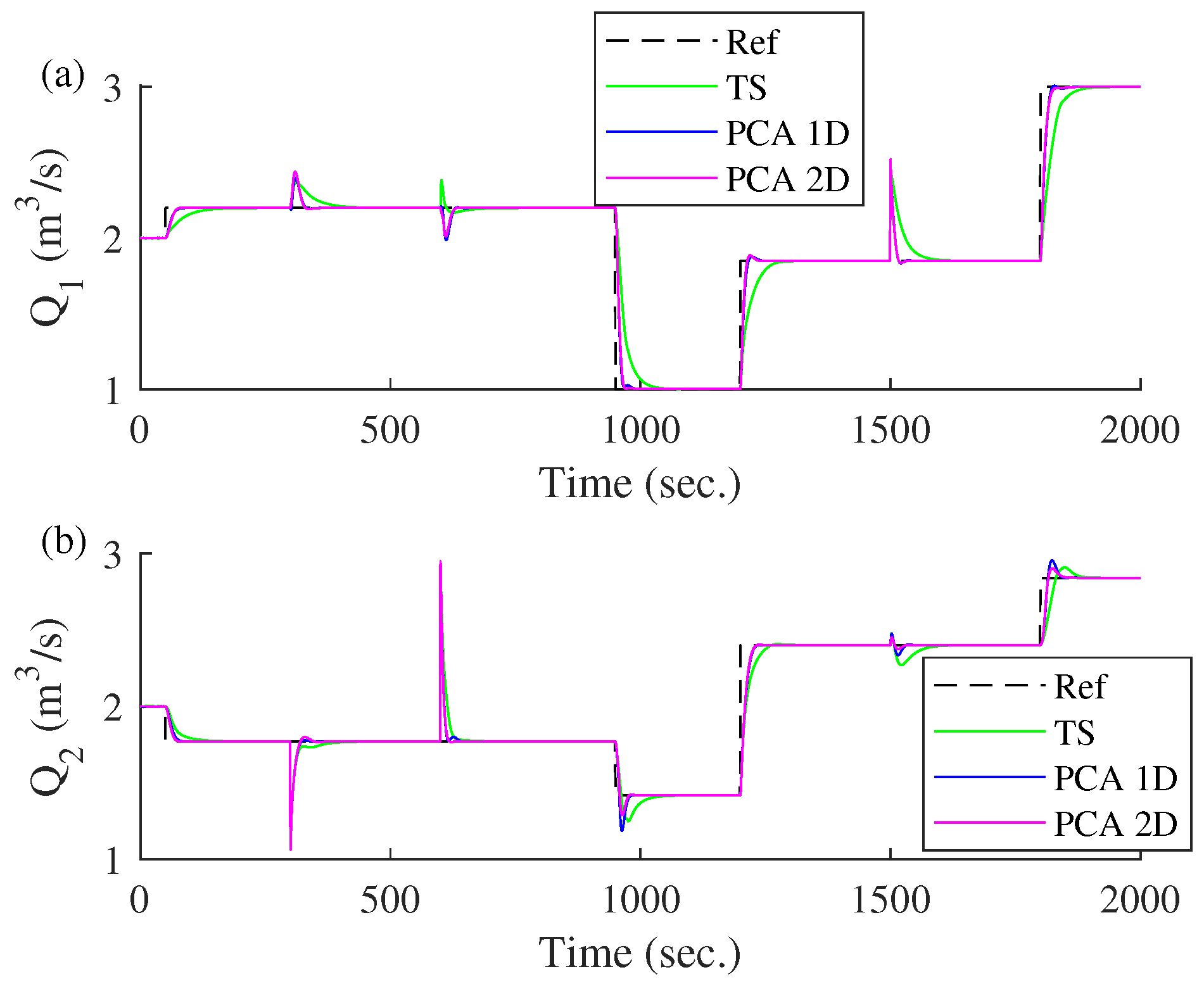
The transient response of the three models with successive steps considered as disturbances is shown in Figure 18, and with consecutive ramps being shown in Figure 19. The changes in both figures are considered disturbance effects because they represent unexpected variations in the reference input: sudden changes in the case of steps and gradual variations in the case of ramps. These disturbances test the system’s ability to handle unpredicted changes in the reference signal.

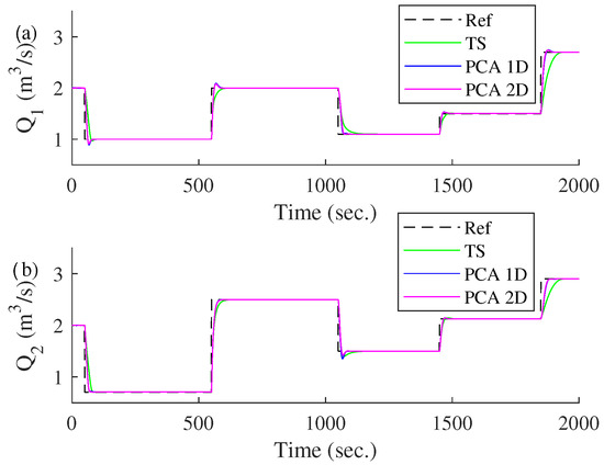
Figure 18. Comparison of different control models based on the incremental approach in front of consecutive steps considered as disturbance in the reference input. (a) Transient response of $Q_1$. (b) Transient response of $Q_2$.

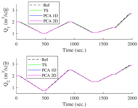
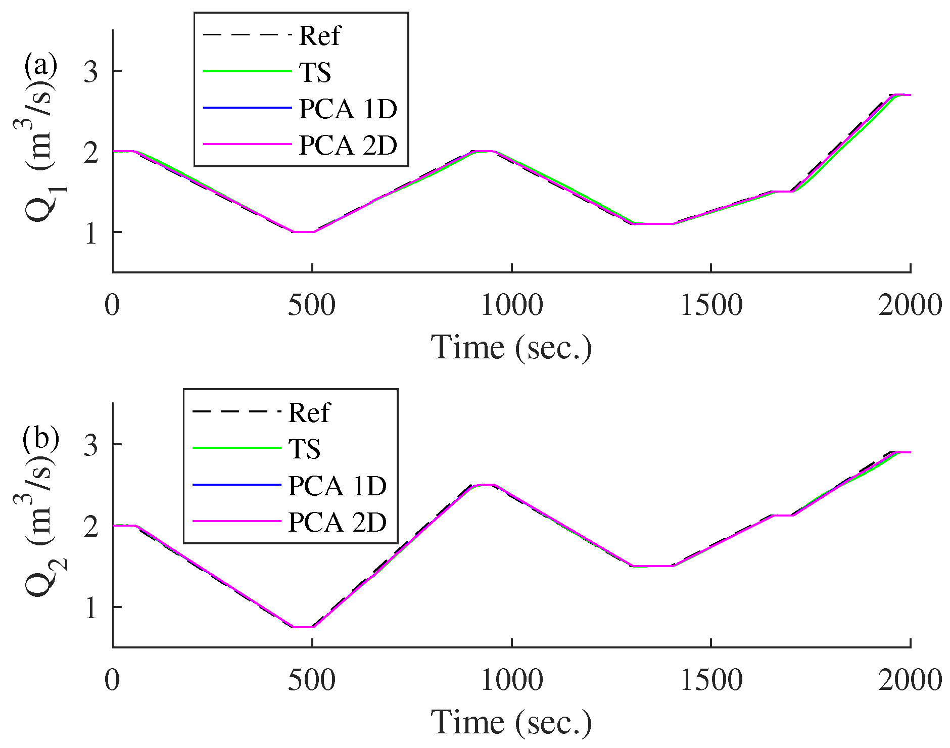
Figure 19. Comparison of different control models based on the incremental approach in front of consecutive ramps considered as disturbance in the reference input. (a) Transient response of $Q_1$. (b) Transient response of $Q_2$.

Furthermore, Figure 20 shows the applied load conditions, where the first load starts at sample 300 when ${\alpha }_2$ is reduced to 0.06 m². After 300 samples, the value returns to the initial one (0.10 m²). Another load occurs in sample 1500 when there is a 15 m increase in the height of tank 1 ($h_1$). Figure 21 shows the transient response of the three models under the load conditions explained above, where the PCA 1D and PCA 2D models present an advantage of fast and smooth transient response in comparison to T–S without PCA.

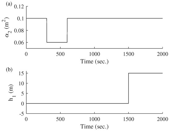
Figure 20. System loads. (a) Load applied to ${\alpha }_2$. (b) Load applied to tank height 1 ($h_1$).

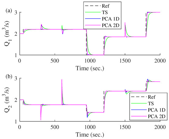
Figure 21. Comparison of different control models based on incremental approach in front of various loads. (a) Transient response of $Q_1$. (b) Transient response of $Q_2$.

However, if the RMSE of each control model is calculated, certain differences between the models appear, as shown in Table 2.

Table 2. Errors made in control models based on incremental state approach.

Control Model	Number of Rules	% Error RMSE in ${\mathit{Q}}_1$	% Error RMSE in ${\mathit{Q}}_2$	Mean of % Error RMSE
Generalized T–S	9	6.9621	4.7403	5.8512
T–S PCA 1D	5	4.8400	4.1510	4.4955
T–S PCA 2D	9	4.8027	4.0703	4.4365

In conclusion, T–S PCA 1D based on increments has two advantages over T–S without PCA: it reduces the number of fuzzy rules and decreases the RMSE. If PCA 1D is compared to PCA 2D, the results are very similar, with the additional advantage of having a lower number of fuzzy rules. However, the disadvantage of PCA 1D is that the RMSE is higher than in PCA 2D.

On the other hand, T–S PCA 2D based on the incremental approach has an advantage over T–S without PCA: it reduces the RMSE. The advantage over PCA 1D is the lower identification error, but the disadvantage is that the number of rules is not reduced compared to T–S without PCA.

5.1.5. Noise in T–S Control Models Based on Incremental Approach and PCA Technique

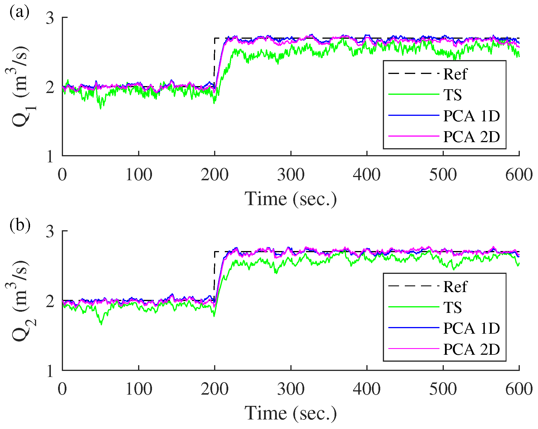
To analyze the behavior of the three control models against noise, a noise of zero mean and 0.01 standard deviation is added to the three output variables ($Q_1$, $Q_2$ and $Q_3$). The output signals obtained by the three controllers are observed in Figure 22. The T–S fuzzy controller that does not use the PCA technique presents difficulties in transient and steady state responses, while the control models that use the PCA technique exhibit a fast and precise steady state response, keeping the output signal around the reference.

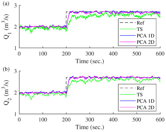
Figure 22. Comparison against noise of controllers based on incremental model. (a) Transient response of $Q_1$. (b) Transient response of $Q_2$.

The mean and standard deviation of the two output variables in the three fuzzy control models based on the incremental approach are summarized in Table 3.

Table 3. Mean and standard deviation of controllers against noise of mean 0 and variance 0.01.

Control Model	Number of Rules	Mean of ${\mathit{Q}}_1$	Standard Deviation of ${\mathit{Q}}_1$	Mean of ${\mathit{Q}}_2$	Standard Deviation of ${\mathit{Q}}_2$
Generalized T–S	9	2.5372	0.0728	2.5894	0.0604
T–S PCA 1D	5	2.6874	0.0286	2.6963	0.0287
T–S PCA 2D	9	2.6596	0.0361	2.7007	0.0333

From the table, it can be concluded that the models implementing the PCA technique (one-dimensional and two-dimensional) perform better against noise than the T–S control model that does not use PCA.

6. Conclusions

In this work, the PCA technique for the control based on fuzzy T–S model was developed. Two different methods were used: PCA 1D and PCA 2D. The first one, PCA 1D, reduces the system’s dimensionality, leading to a decrease in the number of fuzzy rules required within the T–S model. This reduction has simplified the complexity of system variables and has consequently lowered the computational cost of maintaining the accuracy of the incremental state model. PCA 2D provides a fast and smooth transient response in front of disturbances and loads in comparison to the T–S model without PCA. Moreover, models that use the PCA technique, both in one- and two-dimensional forms, demonstrate superior performance in handling noise compared to the T–S control model, which does not incorporate PCA. The effectiveness of both PCA methods was validated using an interconnected double-tank system, demonstrating its ability to maintain control accuracy while minimizing the computational cost.

References

- Zadeh, L. Fuzzy sets. Inf. Control 1965, 8, 338–353. [Google Scholar] [CrossRef]
- Adánez, J.; Al-Hadithi, B.M.; Jiménez, A. Multidimensional membership functions in T–S fuzzy models for modelling and identification of nonlinear multivariable systems using genetic algorithms. Appl. Soft Comput. 2019, 75, 607–615. [Google Scholar] [CrossRef]
- Tang, G.; Yang, M.; Liu, Q.; Yang, S. Design of an Adaptive Fuzzy Sliding Mode Controller for Hydraulic Position Servo System. In Proceedings of the 2023 IEEE 12th Data Driven Control and Learning Systems Conference (DDCLS), Xiangtan, China, 12–14 May 2023; pp. 1239–1244. [Google Scholar]
- Chen, L.; Gao, J. Adaptive Sliding Mode Control for Automotive Electronic Throttle based on Extremum Seeking. In Proceedings of the 2024 39th Youth Academic Annual Conference of Chinese Association of Automation (YAC), Dalian, China, 7–9 June 2024; pp. 703–708. [Google Scholar]
- Goyal, S.; Deolia, V.K.; Agrawal, S.; Yadav, I. An Adaptive Fuzzy Tuned PID Pitch Controller For Large VSWT Wind Turbine. In Proceedings of the 2024 3rd International Conference on Power Electronics and IoT Applications in Renewable Energy and Its Control (PARC), Mathura, India, 23–24 February 2024; pp. 557–561. [Google Scholar]
- Eltag, K.; Aslamx, M.S.; Ullah, R. Dynamic Stability Enhancement Using Fuzzy PID Control Technology for Power System. Int. J. Control Autom. Syst. 2019, 17, 234–242. [Google Scholar] [CrossRef]
- Dogruer, T.; Can, M.S. Design and robustness analysis of fuzzy PID controller for automatic voltage regulator system using genetic algorithm. Trans. Inst. Meas. Control 2022, 44, 1862–1873. [Google Scholar] [CrossRef]
- Zied Ben Hazem, M.J.F.; Bingül, Z. A Study of Anti-swing Fuzzy LQR Control of a Double Serial Link Rotary Pendulum. IETE J. Res. 2023, 69, 3443–3454. [Google Scholar] [CrossRef]
- Samad, B.A.; Anayi, F.; Melikhov, Y.; Mohamed, M.; Altayef, E. Modelling of LQR and Fuzzy-LQR Controllers for Stabilisation of Multi-link Robotic System (Robogymnast). In Proceedings of the 2022 8th International Conference on Automation, Robotics and Applications (ICARA), Prague, Czech Republic, 18–20 February 2022; pp. 33–38. [Google Scholar]
- Al-Hadithi, B.M.; Jiménez, A.; Perez-Oria, J. New incremental Takagi–Sugeno state model for optimal control of multivariable nonlinear time delay systems. Eng. Appl. Artif. Intell. 2015, 45, 259–268. [Google Scholar] [CrossRef]
- Al-Hadithi, B.M.; Adánez, J.M.; Comina, M.; Jiménez, A. Incremental state model in predictive control: A new fuzzy control proposal for nonlinear systems. IET Control Theory Appl. 2022, 16, 573–586. [Google Scholar] [CrossRef]
- Sánchez, A.; Gallego, A.; Escaño, J.; Camacho, E. Adaptive incremental state space MPC for collector defocusing of a parabolic trough plant. Sol. Energy 2019, 184, 105–114. [Google Scholar] [CrossRef]
- Bouwmans, T.; Javed, S.; Zhang, H.; Lin, Z.; Otazo, R. On the Applications of Robust PCA in Image and Video Processing. Proc. IEEE 2018, 106, 1427–1457. [Google Scholar] [CrossRef]
- Nandini, D.U.; Saravanan, M.; Mayan, J.A.; Kamalesh, M.D.; Prasad, K.M. Automatic traffic control system using PCA based approach. In Proceedings of the 2017 International Conference on Energy, Communication, Data Analytics and Soft Computing (ICECDS), Chennai, India, 1–2 August 2017; pp. 2387–2392. [Google Scholar]
- Kravchik, M.; Shabtai, A. Efficient Cyber Attack Detection in Industrial Control Systems Using Lightweight Neural Networks and PCA. IEEE Trans. Dependable Secur. Comput. 2021, 19, 2179–2197. [Google Scholar] [CrossRef]
- Liu, H. Big data precision marketing and consumer behavior analysis based on fuzzy clustering and PCA model. J. Intell. Fuzzy Syst. 2020, 40, 1–11. [Google Scholar] [CrossRef]
- Ahmadi, M.; Sharifi, A.; Fard, M.J.; Soleimani, N. Detection of brain lesion location in MRI images using convolutional neural network and robust PCA. Int. J. Neurosci. 2023, 133, 55–66. [Google Scholar] [CrossRef] [PubMed]
- Hosseinpour, S.; Martynenko, A. An adaptive fuzzy logic controller for intelligent drying. Dry. Technol. 2023, 41, 1110–1132. [Google Scholar] [CrossRef]
- Zhang, S.; Dubay, R.; Charest, M. A principal component analysis model-based predictive controller for controlling part warpage in plastic injection molding. Expert Syst. Appl. 2015, 42, 2919–2927. [Google Scholar] [CrossRef]
- Saravanan, G.; Suresh, K.; Pazhanimuthu, C.; Senthil Kumar, R. Artificial rabbits optimization algorithm based tuning of PID controller parameters for improving voltage profile in AVR system using IoT. e-Prime Adv. Electr. Eng. Electron. Energy 2024, 8, 100523. [Google Scholar] [CrossRef]
- Hu, G.; You, F. Renewable energy-powered semi-closed greenhouse for sustainable crop production using model predictive control and machine learning for energy management. Renew. Sustain. Energy Rev. 2022, 168, 112790. [Google Scholar] [CrossRef]
- Alves de Araujo Junior, C.A.; Mauricio Villanueva, J.M.; Almeida, R.J.S.d.; Azevedo de Medeiros, I.E. Digital Twins of the Water Cooling System in a Power Plant Based on Fuzzy Logic. Sensors 2021, 21, 6737. [Google Scholar] [CrossRef] [PubMed]
- Takagi, T.; Sugeno, M. Fuzzy identification of systems and its applications to modeling and control. IEEE Trans. Syst. Man Cybern. 1985, SMC-15, 116–132. [Google Scholar] [CrossRef]
- Al-Hadithi, B.; Jimenez, A.; Matía, F. A new approach to fuzzy estimation of Takagi–Sugeno model and its applications to optimal control for nonlinear systems. Appl. Soft Comput. 2011, 12, 280–290. [Google Scholar] [CrossRef]
- Barrientos, A.; Peñín, L.F.; Balaguer, C.; Aracil Santoja, R. Fundamentos de Robótica; McGraw-Hill: London, UK, 2007. [Google Scholar]
- Khalid, M.U.; Kadri, M.B. Liquid level control of nonlinear coupled tanks system using linear model predictive control. In Proceedings of the 2012 International Conference on Emerging Technologies, Islamabad, Pakistan, 8–9 October 2012; pp. 1–5. [Google Scholar]
Disclaimer/Publisher’s Note: The statements, opinions and data contained in all publications are solely those of the individual author(s) and contributor(s) and not of MDPI and/or the editor(s). MDPI and/or the editor(s) disclaim responsibility for any injury to people or property resulting from any ideas, methods, instructions or products referred to in the content. |
© 2025 by the authors. Licensee MDPI, Basel, Switzerland. This article is an open access article distributed under the terms and conditions of the Creative Commons Attribution (CC BY) license (https://creativecommons.org/licenses/by/4.0/).