Transfer Learning for Thickener Control

Abstract

Thickener control is a key area of focus in the minerals processing industry, particularly due to its crucial role in water recovery, which is essential for sustainable resource management. The highly nonlinear nature of thickener dynamics presents significant challenges in modeling and optimization, making it a strong candidate for advanced surrogate modeling techniques. However, traditional data-driven approaches often require extensive datasets, which are frequently unavailable, especially in new plants or unexplored operational domains. Developing data-driven models without enough data representative of the dynamics of the system could result in incorrect predictions and consequently, unstable response of the controller. This paper proposes the application of a methodology that leverages transfer learning to address these data limitations to enhance surrogate modeling and model predictive control (MPC) of thickeners. The performance of three approaches—a base model, a transfer learning model, and a physics-informed neural network (PINN)—are compared to demonstrate the effectiveness of transfer learning in improving control strategies under limited data conditions.

1. Introduction

Thickener processes are integral components in mineral processing, crucial for solid–liquid separation through sedimentation. Effective control of these processes enhances throughput, improves product quality, and reduces operational costs by maintaining a consistent underflow concentration and improving water recovery from the overflow. In practice, up to 80% of the water can be recovered during the thickening stage [1]. However, the complex, nonlinear dynamics of thickeners present significant challenges for traditional control strategies, as slow settling rates introduce response delays, and variable feed conditions lead to nonlinear system behavior that is difficult for feedback controllers to manage, thus resulting in a diluted underflow that affects the quality of the product downstream and additional water waste to tailings.

Solid–liquid separation is an integral component of the mineral processing industry, playing an important role in the recovery of valuable minerals, the use of water resources, and the management of waste. Over the years, a variety of solid–liquid separation technologies have been developed, ranging from simple methods such as filters and sedimentation units to more complex machinery, like hydrocyclones, centrifuges, and flotation cells. Sedimentation units, such as thickeners, are prevalent for large-volume, solid–liquid separation, especially in tailings management and water recovery. Since their invention in 1906, thickeners have supported continuous operations in the gold, copper, iron, coal, nickel, and zinc industries, assisting in cyanide leaching and thickening, flotation concentrate thickening, tailings thickening, water conservation, recovery, effluent treatment, and residue management processes [2]. Furthermore, the understanding of sedimentation theory has enabled innovations in thickener design and operations that have enhanced operational efficiency across industries. The work by Concha and Bürger [2] summarizes the evolution of thickening theory and practice in the past century, highlighting the major contributions that have shaped our understanding of operating variables in a continuous thickening process, kinematic theory of sedimentation, dynamic theory of sedimentation, and thickener design, which have in turn enabled innovations such as high-rate, and high-capacity thickeners.

This paper contributes to the development of more efficient thickener operations by presenting a methodology for data-driven control. Namely, the use of neural networks and transfer learning techniques is presented as a method to leverage large amounts of data from a thickener to model and control a different thickener with a similar design but different operating conditions.

1.1. Continuous Thickener Modeling

The cornerstone of dynamic modeling of thickeners is the work of Kynch [3], which introduces a framework for modeling particle settling velocity as a function of volume fraction $\varphi$. This framework assumes one-dimensional settling in a quiescent medium, where the settling velocity depends on the local suspension concentration. As shown in Equation (1), $\varphi$ represents local concentration, which varies as a function of space x and time t, while $f_{bk}$ is the Kynch batch flux density function, capturing effects of particle concentration and settling velocity.

$${\displaystyle \frac{\partial \varphi }{\partial t}}+{\displaystyle \frac{\partial f_{bk}\left(\varphi \right)}{\partial x}}=0$$

(1)

Important advancements in dynamic sedimentation theory, that build upon the work of Kynch, include the work by Diehl [4], where a nonlinear scalar conservation law is introduced to model the continuous feed of suspension into the thickener, effectively extending Kynch’s theory of sedimentation to account for continuous operation. Equation (2) summarizes the conservation law, where $\delta$ is the Dirac measure, and the flux function $F(u,x)$ is discontinuous at the feed or outlet locations in x. Furthermore, the authors present how the source term and the discontinuities of F can be converted into boundary functions to define a concentration profile.

$${\displaystyle \frac{\partial \varphi (x,t)}{\partial t}}+{\displaystyle \frac{\partial }{\partial x}}\left(F\left(\varphi \right(x,t),x)\right)=s\left(t\right)\delta \left(x\right),$$

(2)

The work by Bürger and Concha [5] further extends the sedimentation model to account for fluctuated suspensions, introducing definitions for hindered settling, compressibility of the sediment bed, and thickener geometry. The model is formulated as a nonlinear partial differential equation (PDE) as shown in Equation (3), where $S\left(x\right)$ is a spatial variation factor to account for thickeners with varying geometry (e.g., conical thickeners), $Q_D\left(t\right)$ is the discharge volumetric flow rate, and $A\left(\varphi \right)$ represents a nonlinear function for diffusivity to account for pressure-driven particle interactions, and captures the effects of particle compression and hindered settling within the sediment bed, allowing for a more accurate representation of sedimentation dynamics in thickeners with varying geometries.

$${\displaystyle \frac{\partial \left(S\right(x\left)\varphi \right)}{\partial t}}+{\displaystyle \frac{\partial }{\partial x}}\left(Q_D\left(t\right)\varphi +S\left(x\right)f_{blk}\left(\varphi \right)\right)={\displaystyle \frac{\partial }{\partial x}}\left(S\left(x\right){\displaystyle \frac{\partial A\left(\varphi \right)}{\partial x}}\right),$$

(3)

In addition to the extended formulation of Kynch’s theory, the authors present constitutive equations for the hindered settling velocity and effective solid stress as functions of local solids concentration, along with high-resolution finite difference schemes for numerically solving the partial differential equation in the steady state. Recent work has further expanded these models to account for additional parameters such as flocculation effects [6,7].

1.2. Thickener Simulation and Control

The seminal work by [3,4,5] and others [8,9,10], has laid the foundation for model-based control of thickeners. Some examples include the work of Betancourt et al. [11], where mathematical models presented by Bürger et al. [12] are used for the simulation and formulation of three Proportional–Integral (PI) controllers that are robust to disturbances (variations in the feed concentration) and can produce a low overflow concentration, and a stable discharge concentration. Another example includes the work by Xu et al. [13], where an intelligent control strategy for thickener underflow and flocculant is presented. The control strategy assumes online measurement of operational parameters including flow rate, mud bed level, and underflow concentration. This approach is validated in a wastewater treatment plant to demonstrate control and a stable underflow concentration. Another example is the work of Yao et al. [14], where a dynamic model is developed and a control strategy with a switching output mechanism is adopted to efficiently handle variable bed heights. The control strategy is demonstrated in three simulated case studies of a thickener operating under conventional conditions.

Other recent examples include the work of Oulhiq et al. [15], where a model predictive control is developed based on a linear vector auto-regressive with exogenous variables (VARX) model. One notable contribution in this work is the incorporation of state variables such as turbidity, rake torque, and cone pressure, additional to the underflow slurry density, which is the primary controlled variable. The control strategy is then demonstrated in an industrial case, resulting in an average error reduction of up to 90% compared to the existing control at the site. In a similar example, Tan et al. [16] present an MPC approach based on linear and extended Kalman filters, and demonstrate their use in an industrial case study that improves operational efficiency of a paste thickener.

1.3. Thickener Simulation and Control with Data-Driven Methods

Although breakthrough developments in sedimentation theory have enabled more sophisticated modeling and control of thickeners, the computational cost and the complexity of these models remain an operational challenge for several factors. First, the thickening process is highly nonlinear, with large delays in the control response, making it challenging even for model-based control strategies to maintain robust control of the underflow concentration. Second, the universally accepted models for continuous sedimentation remain very complex. The flux conditions are usually assumed to be piecewise differentiable [11], with the settling velocity expressions being nonlinear functions of concentration and often modeled using empirical relations [17]. Models that incorporate sediment compressibility effects use additional constitutive relationships that result in higher-order parabolic PDEs, increasing computational complexity. Finally, the computational cost of incorporating spatial discretization scales with finer mesh requirements. All these factors increase the complexity and requirements for stability and convergence of a numerical solution and usually call for the use of iterative solvers.

These challenges have motivated the development of data-driven methods for modeling and control of thickeners. Some examples include the work of Diaz et al. [18], where a Random Forest method is used to model a paste thickener and incorporate it into an MPC scheme that uses evolutionary optimization methods. In a similar example, Jia and You [19] present a data-driven robust model predictive control (DRMPC) that uses a discrete-time linear time-invariant (LTI) model and pressure sensor information to estimate the future states of the thickener, aided by the use of principal component analysis (PCA) to quantify the uncertainty from historical data. The resulting controller, which uses an affine disturbance feedback (ADF) technique, is demonstrated in both simulated and industrial case studies.

Other notable examples include the work of Yuan et al. [20], where a Dual-Attention Recurrent Neural Network was employed to predict the underflow concentration of a thickener using data from multiple sensors, achieving up to a 10% reduction in prediction error compared to other time series models. Similarly, Lei and Karimi [21] utilized a deeply efficient long short-term memory (DE-LSTM) network to predict concentration in a deep cone thickener, comparing its performance against traditional models such as SVM, GRU, and XGBOOST. Furthermore, Yuan et al. [22] proposed a network architecture featuring an encoder-decoder structure and a derivative module to learn the deterministic state-space model of a continuous thickening system, validating their approach through an industrial case study. Additional recent examples include the work by [23,24,25].

1.4. Transfer Learning in Process Control

Data-driven approaches have demonstrated promising results; however, complex architectures such as neural networks typically require substantial amounts of operational data to accurately capture the dynamics of the sedimentation process. This can be a challenge when data are scarce, of poor quality, or not representative of the desired operational conditions of the thickener. This paper introduces the application of transfer learning, a concept originating from machine learning, which leverages knowledge from related systems to enhance modeling and control. In process control, it offers a promising approach to address data scarcity and improve model generalization. Furthermore, in this study, transfer learning is enhanced with the use of a Physics-Informed Neural Network (PINN) that increases the model’s generalization capabilities beyond the known operational domain. The details of this methodology have been presented by the authors in previous publications [26]. For completeness, a brief summary of the approach is presented here.

For a formal definition of transfer learning, let $D_S=\{X_S,Y_S\}$ represent the source domain, where $X_S\in {\mathbb{R}}^m$ denotes the input features and $Y_S\in {\mathbb{R}}^n$ represents the corresponding outputs, with a system model $f_S:X_S\to Y_S$. The task in the source domain is to predict $Y_S$ from $X_S$. Similarly, $D_T=\{X_T,Y_T\}$ denotes the target domain with model $f_T:X_T\to Y_T$ [27].

In conventional machine learning, $f_S$ and $f_T$ are learned independently. However, transfer learning leverages knowledge from $f_S$ (such as pre-trained weights and model parameters) to accelerate and enhance the learning process for $f_T$. The objective of transfer learning can be formulated as follows:

$$\underset{{\theta }_T}{min}{\mathbb{E}}_{(x_T,y_T)\sim D_T}\left[\mathcal{L}(f_T(x_T;{\theta }_T),y_T)\right]\mathrm{where}{f}_T=g(f_S,{\theta }_T)$$

(4)

where ${\theta }_T$ represents the parameters specific to the target domain, and g is a transfer function that incorporates knowledge from the source model $f_S$. Thus, the model $f_S$ from the source domain supports improving the target model $f_T$, typically by initializing parameters or transferring knowledge of the feature space, where ${\theta }_T$ are the parameters of the target model and $L_{\mathrm{data}}$ is the data-driven loss function.

$$\underset{{\theta }_T}{min}{\mathbb{E}}_{(x_T,y_T)\sim D_T}\left[L_{\mathrm{data}}(f_T(x_T;{\theta }_T),y_T)\right],$$

(5)

Furthermore, in this study, knowledge about the process is used to regularize the learning. This is achieved by incorporating physical laws as part of the loss function (e.g., Physics-Informed loss) to the training objective. Assuming F is a differential operator representing the physical laws governing the system:

$$F\left(f_T(x;{\theta }_T)\right)=0,x\in \Omega ,$$

(6)

where $\Omega$ is the domain of interest and $f_T(x;{\theta }_T)$ approximates the system states or outputs. The total loss function $L_{\mathrm{total}}$ then combines the data-driven loss and the physics-based loss:

$$L_{\mathrm{total}}=L_{\mathrm{data}}+\lambda L_{\mathrm{physics}},$$

(7)

where $\lambda$ is a weighting factor balancing the two loss terms. To incorporate transfer learning into the PINN framework, we utilize the weights and parameters from the source model $f_S$ to initialize or inform the target model $f_T$. We can initialize ${\theta }_T$ using the parameters from the source model ${\theta }_S$:

$${\theta }_T={\theta }_S+\Delta \theta ,$$

(8)

where $\Delta \theta$ captures the adjustments needed for the target domain. The optimization problem becomes the following:

$$\underset{{\theta }_T}{min}{L}_{\mathrm{total}}=\underset{{\theta }_T}{min}\left[L_{\mathrm{data}}+\lambda L_{\mathrm{physics}}\right],$$

(9)

In this study, physics-informed transfer learning is utilized to guide the learning process in target systems with limited data availability. The approach leverages extensive data from a similarly designed thickener, which operates under a broader range of conditions, to improve the control of the target system. PINNs offer specific advantages for this process by embedding the governing equations of the target thickener’s dynamics directly into the learning framework. PINNs enhance generalization by enforcing physically consistent behavior, reducing the risk of overfitting to the source data or mismatching predictions in the target domain. Additionally, they require less target domain data compared to traditional data-driven approaches, as the embedded physics compensate for the lack of training examples by constraining the solution space to physically plausible outcomes.

2. Methodology

This paper follows the universally accepted models for dynamic modelling of thickeners, as developed by [4] and Bürger et al. [12], following the empirical expressions and guidelines for parameters selection presented by Bürger and Narváez [8].

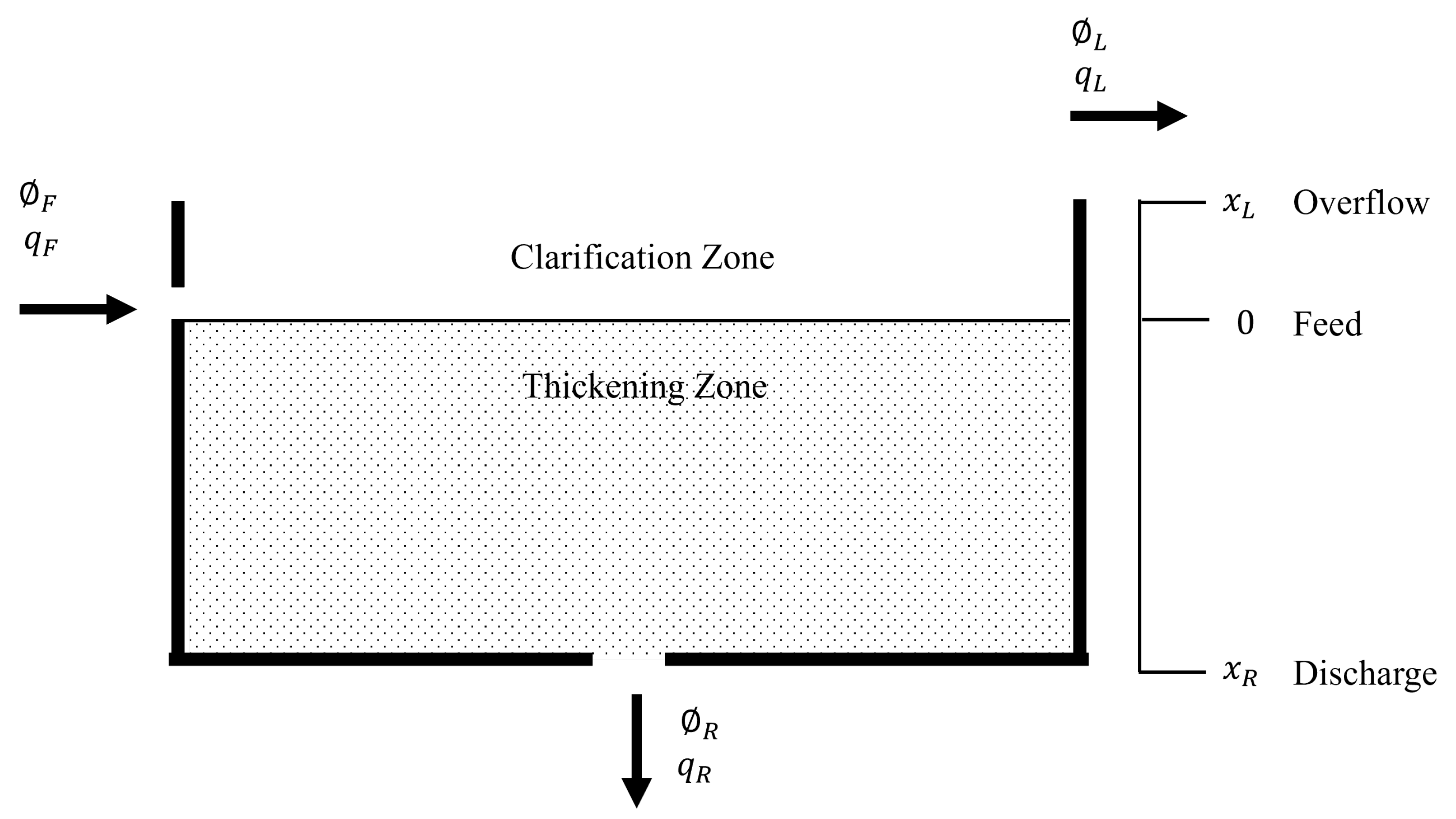
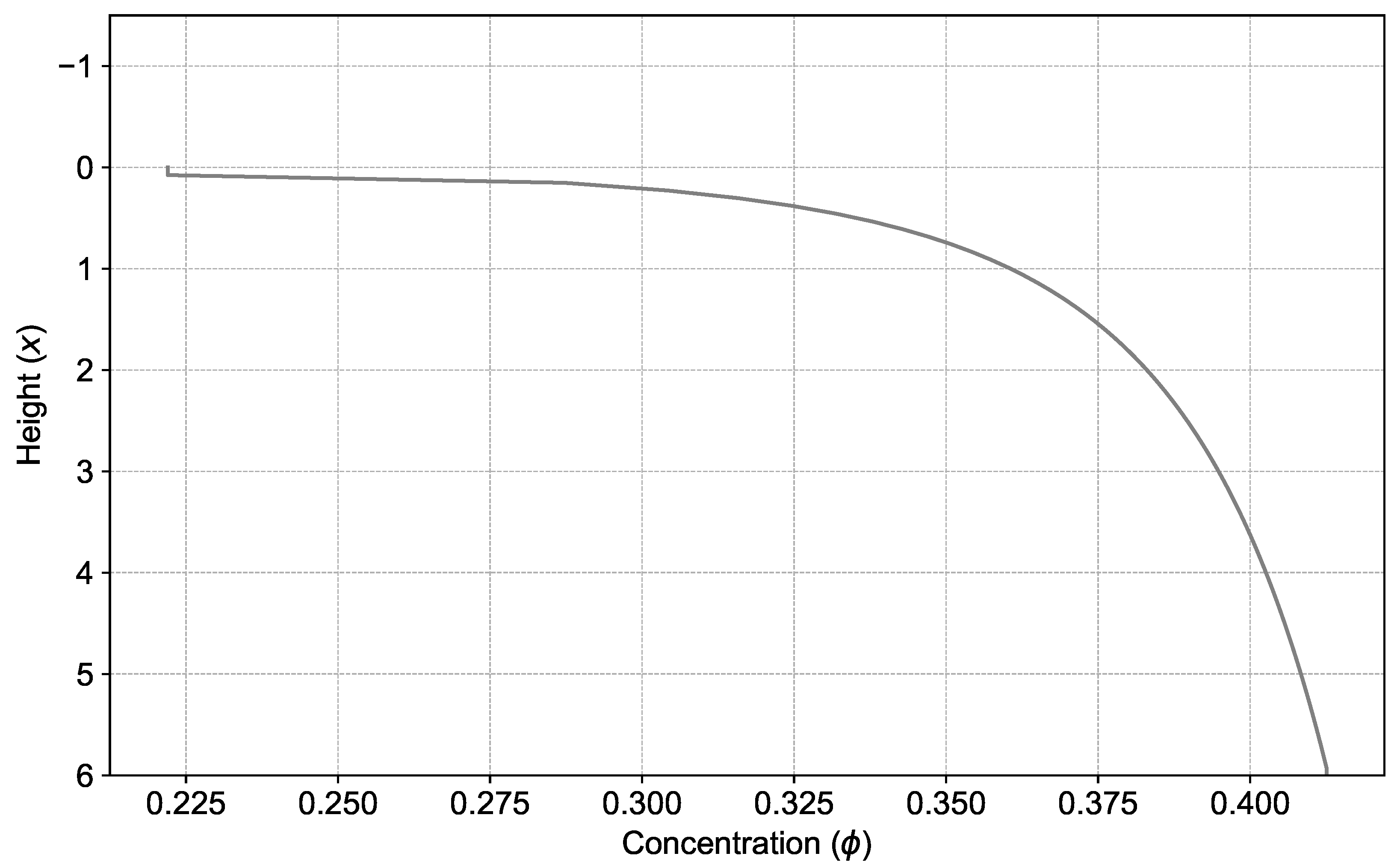
2.1. Thickener Modeling

As presented by [8], Equation (3) can be reduced to the following second-order partial differential equation:

$${\displaystyle \frac{\partial \varphi }{\partial t}}+{\displaystyle \frac{\partial f_{bk}\left(\varphi \right)}{\partial x}}={\displaystyle \frac{{\partial }^{2}A\left(\varphi \right)}{\partial x^2}},$$

(10)

And for a one-dimensional thickener:

$$A\left(\varphi \right):={\int }_0^{\varphi }a\left(s\right)ds,a\left(\varphi \right):={\displaystyle \frac{f_{bk}\left(\varphi \right){\sigma }_{ϵ}\left(\varphi \right)}{\Delta \rho g\varphi }},$$

(11)

where $\Delta \rho g\varphi$ is the solid-fluid density difference and g the gravitational acceleration. Furthermore, functions for the effective solids stress ${\sigma }_e\left(\varphi \right)$ and its derivative ${\sigma }_e^{\prime }\left(\varphi \right)$ satisfy the conditions below at the critical concentration ${\varphi }_c$ point:

$${\sigma }_e\left(\varphi \right),{\sigma }_e^{\prime }\left(\varphi \right)=\left\{\begin{array}{cc}0\hfill & \mathrm{for}\varphi \le {\varphi }_c,\hfill \\ >0\hfill & \mathrm{for}\varphi >{\varphi }_c,\hfill \end{array}\right.$$

(12)

As noted by [8], Equation (10) is a strongly degenerate parabolic PDE, and its solutions are generally discontinuous, thus requiring an entropy condition or selection criterion to identify physically relevant solutions. The details of the steady-state solution to Equation (10) are not discussed in this study, but they can be referenced in the work of Bürger and Narváez [8].

The constitutive relationships, and parameters for the thickener in this study (Figure 1), also follow the approach by Bürger and Narváez [8]. Namely, the empirical form for the flux function, follows the semi-empirical expressions proposed by Richardson and Zaki [17]:

$$f_{bk}\left(\varphi \right)=\left\{\begin{array}{cc}{v}_{\infty }\varphi {(1-\varphi /{\varphi }_{\max })}^N\hfill & \mathrm{for}0\le \varphi \le {\varphi }_{\max },\hfill \\ 0\hfill & \mathrm{otherwise}.\hfill \end{array}\right.$$

(13)

and Equation (14)

$${\sigma }_e\left(\varphi \right)=\left\{\begin{array}{cc}0\hfill & \mathrm{for}\varphi \le {\varphi }_c,\hfill \\ {\alpha }_{1}exp\left({\alpha }_2\varphi \right)\hfill & \mathrm{for}\varphi >{\varphi }_c,\hfill \end{array}\right.$$

(14)

The details on the steady-state solutions or numerical discretization are not discussed in this study, but they have been discussed in detail in the literature [11,12,14]. Figure 2 shows the resulting steady-state profile for a thickener with $x_R=6\mathrm{m}$, $v_{\infty }=6.025\times {10}^{-4}\mathrm{m}/\mathrm{s}$, $N=12.59$, ${\alpha }_1=5.35$, ${\alpha }_2=17.9\mathrm{Pa}$, $\Delta \rho =1650{\mathrm{kg}/\mathrm{m}}^3$, ${\varphi }_c=0.2$, and ${\varphi }_{\max }=0.6$.

The source system in this study corresponds to a thickener under a nominal feed concentration of ${\varphi }_F=0.13$, simulated in an open loop, with underflow pump speed values sampled randomly from a uniform distribution within 20% of the nominal value. Figure 3 shows an example of the simulated source system. The gathered data is then used to train a transformer network to predict underflow concentration values, and the resulting weights of the model are used to initialize other transformer models for the target systems.

To demonstrate the transfer learning methodology, 50 target systems are simulated in this study, each with a different value of ${\varphi }_F$ sampled randomly within 20% of the nominal value used in the source system. While the source system simulation spans more than $3\times {10}^7$ s with multiple changes in pump speed, the target systems are only simulated for $3\times {10}^5$ s with two changes in pump speed (doublet test). The target systems are then evaluated in three different system identification scenarios. In the first scenario, a transformer network is used to model the target thickener. In the second scenario, the weights from the transformer model developed for the source system are used to initialize a transformer network for the target system and train the network with target data. Finally, in the third scenario, the weights from the transformer model are used to initialize a transformer network, but a PINN regularization is used to guide the learning from the target data. The three models for each target system are used for an MPC test example, and their performance is compared.

2.2. Transfer Learning

The first step in this transfer learning demonstration is to measure the similarity between the source and the target system. As pointed out by [28], in situations when the source domain and the target domain differ from each other, transfer learning can fail, and in some cases even hurt the performance resulting in negative transfer. In this study, the similarity between the source and target domain is measured using Dynamic Time Warping (DTW) [29], a well-known algorithm to measure similarity between time series. Figure 4 shows the similarity between the source system and the target systems, suggesting that mitigation might be required to guide the training for target systems with values of ${\varphi }_F$ near the extremes of the spectrum.

2.2.1. Transformer Model

To generate an initial model for transfer learning, the data from the source system is used to train a transformer network. The attention mechanism in transformers offers significant advantages in modeling dynamic processes with long delays by enabling the model to focus on the most relevant parts of the input sequence at each time step.

In processes such as thickeners, where actions and their effects are separated by substantial time lags, traditional modeling methods often struggle to accurately capture these delayed dependencies. The attention mechanism addresses this challenge by assigning different levels of importance to various time steps, allowing the model to effectively account for long-range dependencies while retaining crucial information [22]. The transformer architecture used in this paper is summarized in

Table 1. Transformer-based model architecture summary with detailed specifications for each layer.

Layer Type	Details
Input Layer	Shape: (window = 5, features: 2)
Multi-Head Attention (1st block)	10 heads, key_dim = 2; Residual connection with input
Dense Layer	100 units, tanh activation
Dropout	0.2 dropout rate
Dense Layer	Output units: n_feature, no activation
Multi-Head Attention (2nd block)	10 heads, key_dim = 2; Residual connection with input
Dense Layer	100 units, tanh activation
Dropout	0.2 dropout rate
Dense Layer	Output units: features: 2, no activation
Flatten	Flatten the output
Output Layer	Dense layer, units: n_label, linear activation

. Figure 5 shows the results from training the transformer network with source system data.

To evaluate the performance of the resulting transformer model in the control application, the model is implemented within an MPC. The control problem is initialized from a steady state, followed by a setpoint change corresponding to a 10% increase in the underflow concentration. This serves as a benchmark, demonstrating that the transformer model, when trained with sufficient data, exhibits strong performance in the MPC application. In this MPC setup, the thickener system dynamics are captured using two models: a first-principles model for simulation and a data-driven model for prediction. The simulation provides an accurate representation of the process dynamics, whereas the data-driven model estimates future states based on historical data. The MPC aims to minimize a quadratic objective function representing the error between the predicted output and the setpoint while penalizing control moves, as shown in Equation (15):

$$\underset{u}{min}\sum _{k=0}^{P-1}{\left(\widehat{y}(t+k)-y_{\mathrm{set}}(t+k)\right)}^2+\lambda \sum _{k=0}^{M-1}\Delta u{(t+k)}^2$$

(15)

where P is the prediction horizon, M is the control horizon, $\widehat{y}(t+k)$ is the predicted output by the transformer model, $y_{\mathrm{set}}(t+k)$ is the setpoint, $\Delta u(t+k)$ is the control move, and $\lambda$ is a tuning parameter that penalizes aggressive control actions. Figure 6 shows the result of the MPC.

In applying transfer learning within this study, the original data-driven models are replaced with models incorporating transfer learning. Two approaches are examined: the first involves initializing the model with target system data followed by retraining, while the second utilizes the same initialization and retraining process but incorporates a PINN regularization in the loss function to guide the learning process.

2.2.2. Transfer Learning Models

The transformer model trained on the source data is employed for transfer learning on the target systems and evaluated under two distinct scenarios. In the first scenario, the network architecture and weights of the source model are transferred to initialize a transformer network, which is then retrained using target system data. In this case, only the final layer is retrained, while the remaining layers are frozen, preserving the knowledge from the source model. It is important to note that less than 5% of the target data, relative to the total source data, is used to retrain the target models. This approach highlights the potential of transfer learning in scenarios where process data is limited, such as during plant startup.

In the second scenario, the network architecture and weights of the source model are similarly transferred to initialize the transformer network. However, a regularization term based on a PINN is introduced to guide the learning process. The same target data used in the first scenario is employed here, but the addition of the PINN regularization—derived from first-principles equations—improves learning. This regularization term could be adapted to represent other aspects of the process, including historical or synthetic data, broadening the applicability of the method.

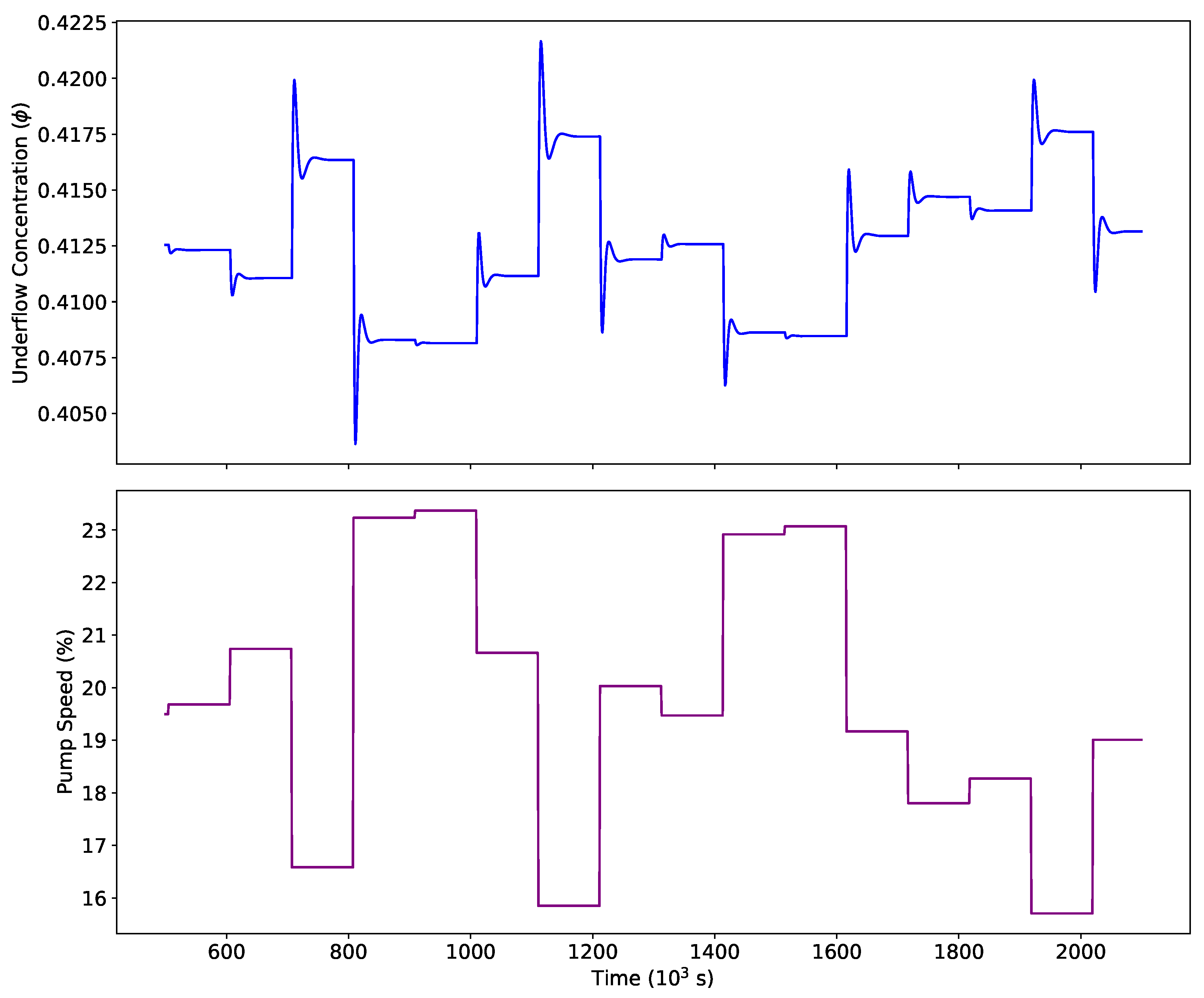
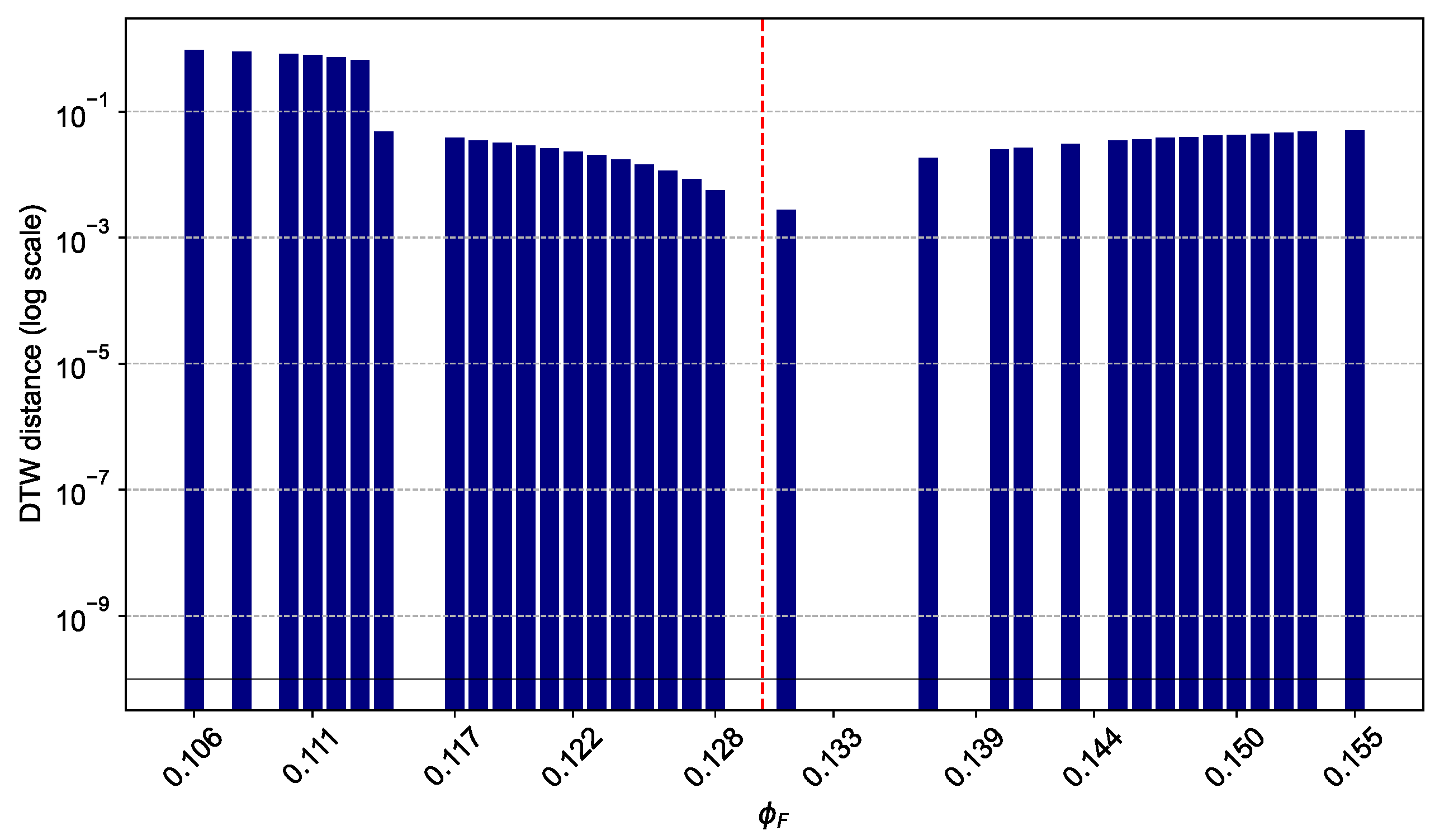
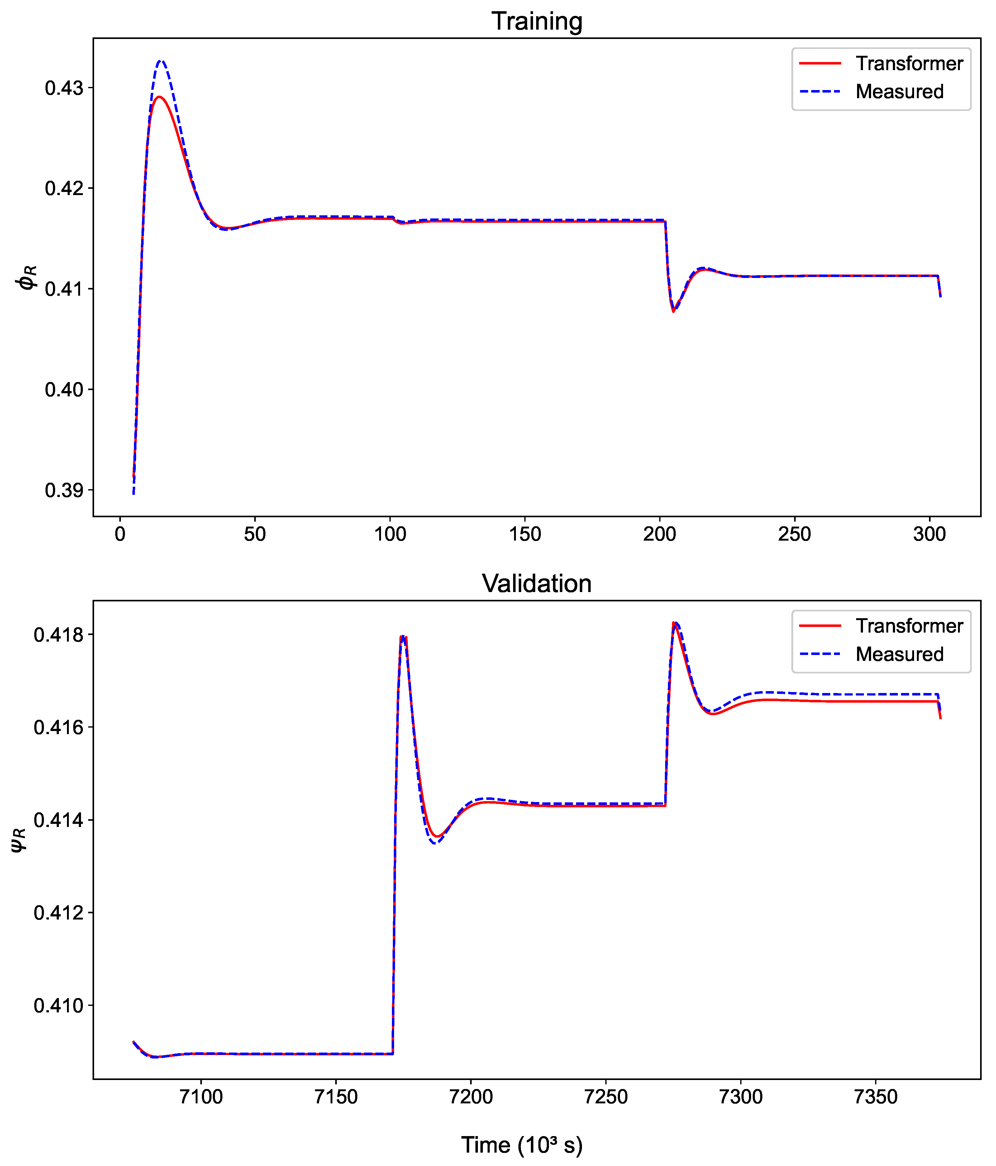
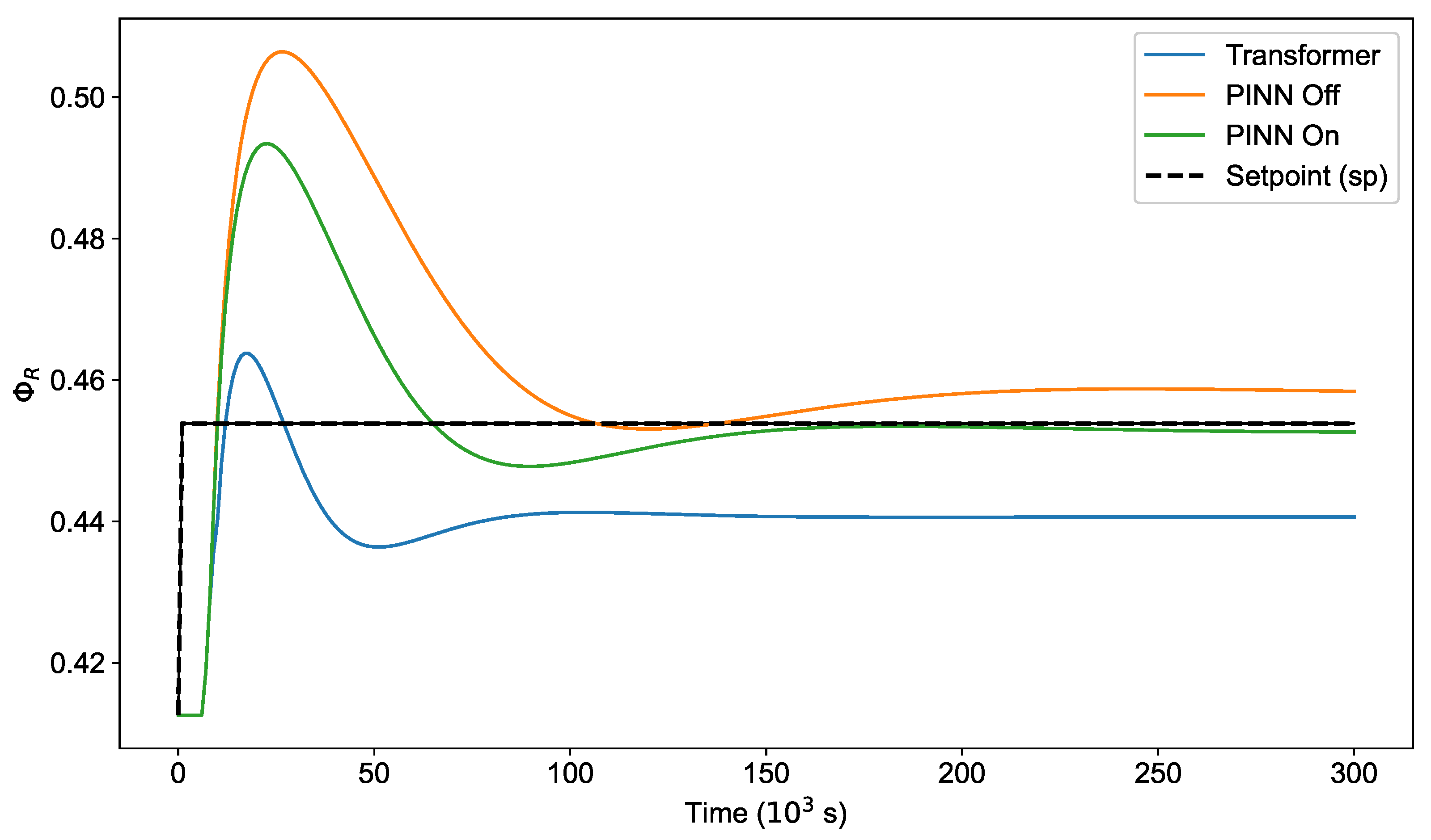
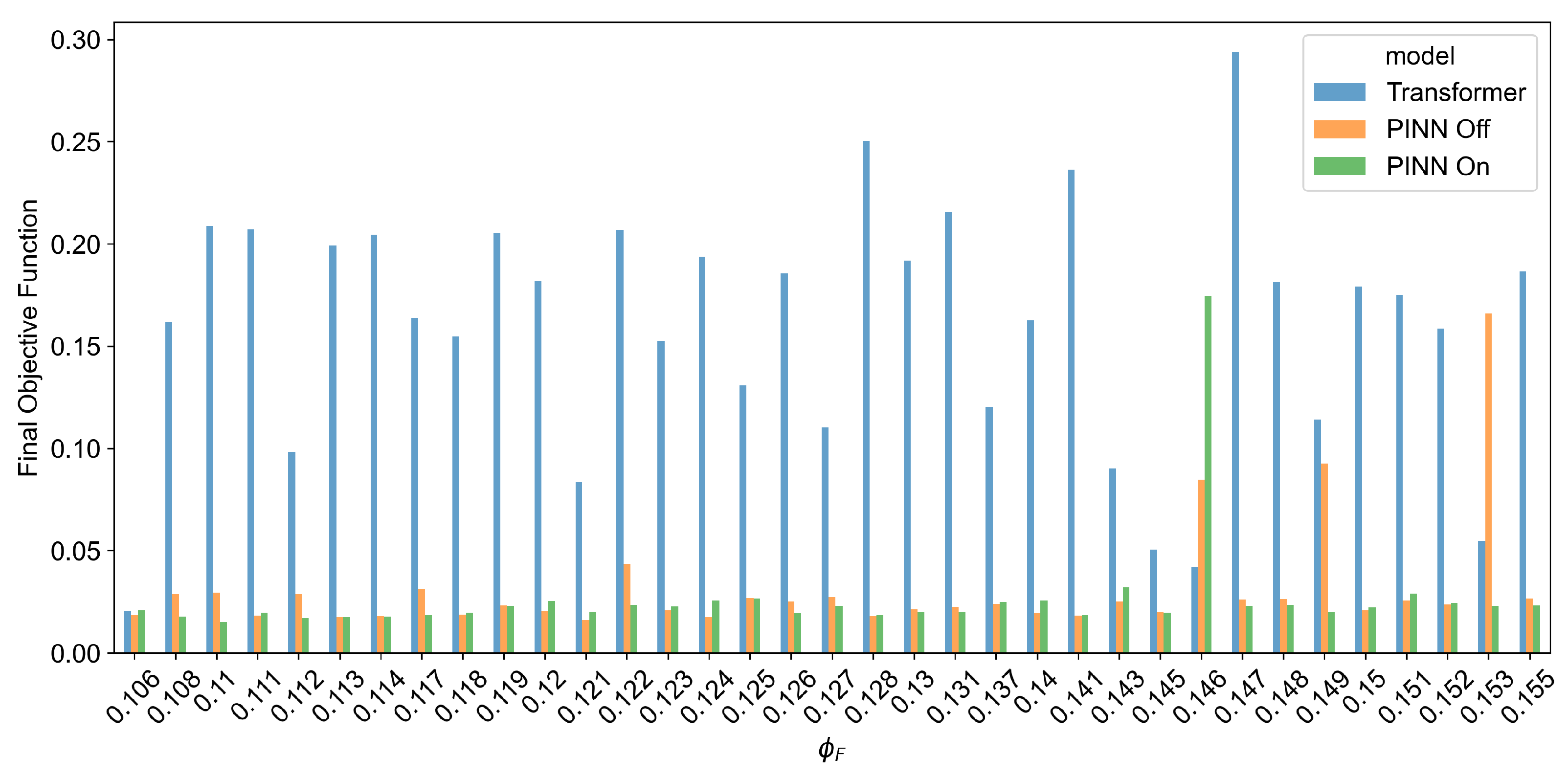
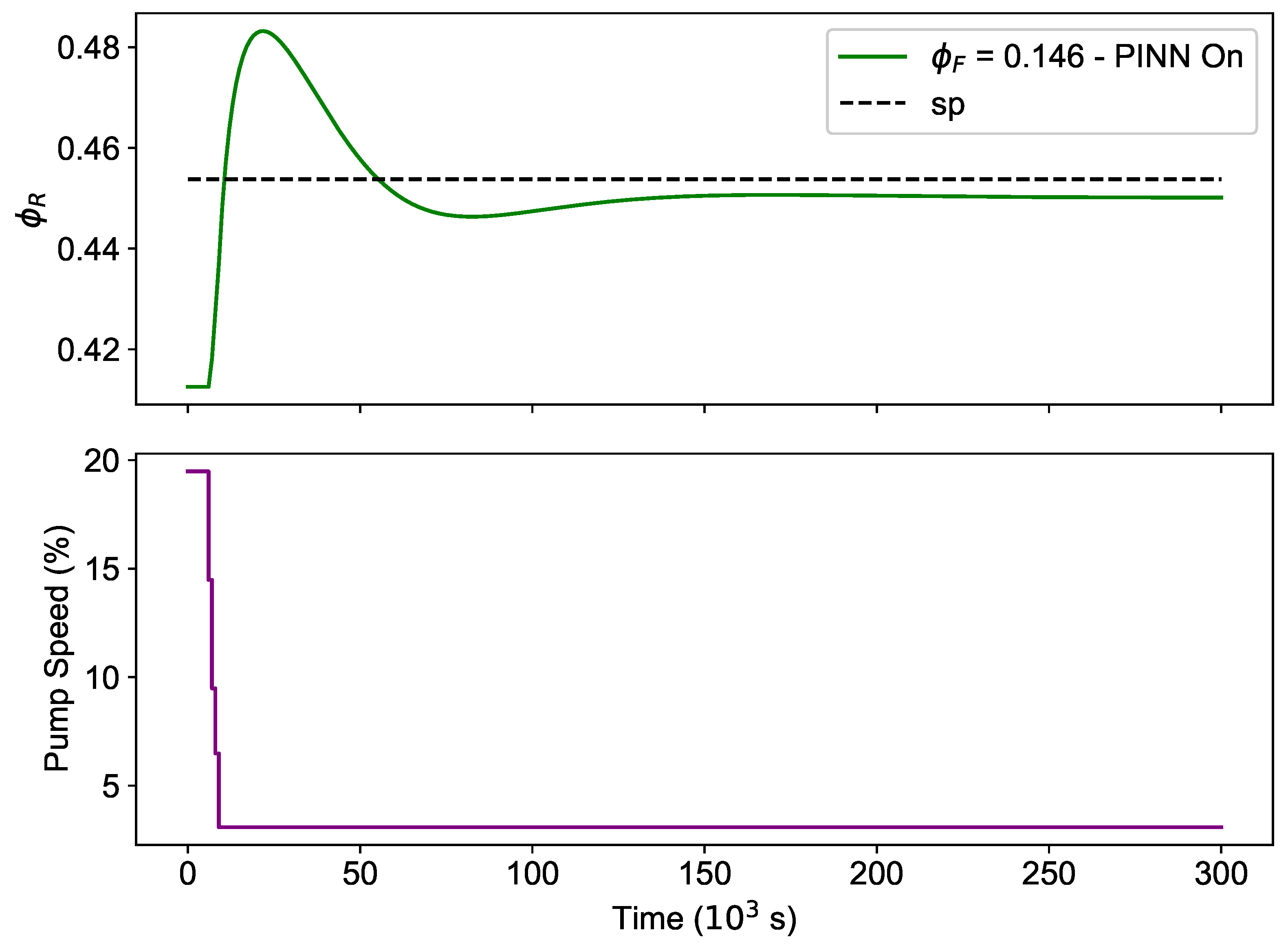
3. Results and Discussion

As discussed earlier, the models are employed to make predictions within an MPC framework and are tested in a simulation of a thickener with a first-principles model, where the setpoint is increased by 10% from the steady-state value. Figure 7 illustrates the performance of these models under such conditions. The results indicate that the model utilizing transfer learning provides superior performance compared to the transformer trained solely on target data. Specifically, an improvement of 87% is achieved with transfer learning, while an additional improvement of 99% is observed when PINN regularization is introduced.

Figure 8 presents the results of applying the transfer learning methodology to 50 target systems. Overall, the models trained using the transfer learning approach consistently outperformed those trained exclusively on target data.

Note that there are cases in which the error is high even for the transfer learning approach, such as for some values of ${\varphi }_F>145$. This highlights the nonlinearity of the process and instances where the control fails to converge to the setpoint despite transfer learning. This suggests a need for additional tuning of the MPC parameters or indicates a limitation of the mathematical model used to represent the thickener. Figure 9 shows the resulting performance of the MPC after further tuning of the prediction and control horizon lengths.

Additionally, it is worth noting that, in certain instances, models trained without PINN slightly outperform those incorporating PINN. This can be attributed to the fact that Figure 8 displays the average error between the setpoint and the process over the entire duration of the simulation. Figure 10, on the other hand, presents the average error across all simulations at each point in time, showing that the PINN model exhibits a higher error at the onset of the setpoint change but eventually stabilizes to a lower error.

This behavior suggests that the PINN model provides a more accurate representation of the process, resulting in a lower final error despite a higher initial overshoot. Additionally, the inclusion of PINN regularization results in reduced variation in performance. On average, the PINN-regularized model exhibits 63% less variation compared to the transformer model and 28% less variation compared to the transfer learning model without PINN.

While the results presented here are derived from simulations using first-principles data, the demonstrated process has the potential to be applied to data-driven approaches that have already proven successful in industrial applications. For instance, transfer learning can enhance the accuracy of data-driven models already deployed [22,30] by retraining the models with additional datasets from similar domains. Furthermore, the authors have previously demonstrated the application of transfer learning for developing an approximate MPC [26]. This methodology could improve models designed to infer the control policy rather than model the process itself, as illustrated in the case study presented by [23].

4. Conclusions

In this study, transfer learning was applied to the control of a thickener process within an MPC policy. The results demonstrated that models leveraging transfer learning outperformed the baseline transformer model trained exclusively on target data, with a performance improvement of up to 87%. Furthermore, the incorporation of a Physics-Informed Neural Network (PINN) further increased the accuracy of the control performance, achieving a 99% improvement over the baseline transformer model trained with target data only. These findings underscore the effectiveness of transfer learning in scenarios with limited target data, as well as the benefits of embedding domain knowledge through PINN regularization. Additionally, transfer learning-based models exhibited reduced performance variation compared to models trained solely on target data, further validating their robustness.

However, it was observed that certain conditions, particularly those involving higher values of ${\varphi }_F$, resulted in control errors despite the use of transfer learning. This highlights the nonlinear complexity of the process and suggests that additional tuning of MPC parameters or improvements to the mathematical models may be required to address these scenarios effectively. Fine-tuning of the prediction and control horizon lengths was shown to improve the performance under such challenging conditions, demonstrating the importance of adapting control parameters for specific operating ranges.

This study aims to provide a guideline for future research exploring the application of the proposed methods to a broader range of operating conditions, including industrial case studies. While data-driven models are generally computationally faster than first-principles models, the speed of the MPC optimization subroutine remains dependent on solution feasibility. Although PINNs have shown potential to mitigate this limitation [31], further investigation is needed to optimize the computational efficiency of PINN-regularized transfer learning models and to establish their guarantees for control stability. Such analysis is crucial for assessing their viability in real-time applications. Additionally, extending transfer learning frameworks to include other control strategies or adaptive learning techniques could further enhance robustness and adaptability in practical industrial environments.

References

1. Wills, B.; Finch, J. Wills’ Mineral Processing Technology: An Introduction to the Practical Aspects of Ore Treatment and Mineral Recovery; Butterworth-Heinemann: Waltham, MA, USA, 2016. [Google Scholar]
2. Concha, F.; Bürger, R. Thickening in the 20 th century: A historical perspective. Min. Metall. Explor. 2003, 20, 57–67. [Google Scholar]
3. Kynch, G.J. A theory of sedimentation. Trans. Faraday Soc. 1952, 48, 166–176. [Google Scholar] [CrossRef]
4. Diehl, S. A conservation Law with Point Source and Discontinuous Flux Function Modelling Continuous Sedimentation. SIAM J. Appl. Math. 1996, 56, 388–419. [Google Scholar] [CrossRef]
5. Bürger, R.; Concha, F. Mathematical model and numerical simulation of the settling of flocculated suspensions. Int. J. Multiph. Flow 1998, 24, 1005–1023. [Google Scholar] [CrossRef]
6. Gao, R.; Zhou, K.; Zhang, J.; Guo, H.; Ren, Q. Research on the dynamic characteristics in the flocculation process of mineral processing tailings. IEEE Access Pract. Innov. Open Solut. 2019, 7, 129244–129259. [Google Scholar] [CrossRef]
7. Zhang, L.; Wang, H.; Wu, A.; Yang, K.; Zhang, X.; Guo, J. Effect of flocculant dosage on the settling properties and underflow concentration of thickener for flocculated tailing suspensions. Water Sci. Technol. 2023, 88, 304–320. [Google Scholar] [CrossRef]
8. Bürger, R.; Narváez, A. Steady-state, control, and capacity calculations for flocculated suspensions in clarifier-thickeners. Int. J. Miner. Process. 2007, 84, 274–298. [Google Scholar] [CrossRef]
9. Bustos, M.C.; Concha, F.; Bürger, R.; Tory, E.M.; Bustos, M.C.; Concha, F.; Bürger, R.; Tory, E.M. Theory of sedimentation of ideal suspensions. In Sedimentation and Thickening: Phenomenological Foundation and Mathematical Theory; Springer: Berlin/Heidelberg, Germany, 1999; pp. 27–34. [Google Scholar]
10. Berres, S.; Bürger, R.; Tory, E.M. Applications of polydisperse sedimentation models. Chem. Eng. J. 2005, 111, 105–117. [Google Scholar] [CrossRef]
11. Betancourt, F.; Concha, F.; Sbarbaro-Hofer, D. Simple mass balance controllers for continuous sedimentation. Comput. Chem. Eng. 2013, 54, 34–43. [Google Scholar] [CrossRef]
12. Bürger, R.; Karlsen, K.; Towers, J.D. A Model of Continuous Sedimentation of Flocculated Suspensions in Clarifier-Thickener Units. SIAM J. Appl. Math. 2005, 65, 882–940. [Google Scholar] [CrossRef]
13. Xu, N.; Wang, X.; Zhou, J.; Wang, Q.; Fang, W.; Peng, X. An intelligent control strategy for thickening process. Int. J. Miner. Process. 2015, 142, 56–62. [Google Scholar] [CrossRef]
14. Yao, Y.; Tippett, M.; Bao, J.; Bickert, G. Dynamic Modeling of Industrial Thickener for Control Design; Engineers Australia: Barton, Australia, 2012. [Google Scholar]
15. Oulhiq, R.; Benjelloun, K.; Kali, Y.; Saad, M.; Griguer, H. Constrained model predictive control of an industrial high-rate thickener. J. Process Control 2024, 133, 103147. [Google Scholar] [CrossRef]
16. Tan, C.K.; Bao, J.; Bickert, G. A study on model predictive control in paste thickeners with rake torque constraint. Miner. Eng. 2017, 105, 52–62. [Google Scholar] [CrossRef]
17. Richardson, J.; Zaki, W. The sedimentation of a suspension of uniform spheres under conditions of viscous flow. Chem. Eng. Sci. 1954, 3, 65–73. [Google Scholar] [CrossRef]
18. Diaz, P.; Salas, J.C.; Cipriano, A.; Núñez, F. Random forest model predictive control for paste thickening. Miner. Eng. 2021, 163, 106760. [Google Scholar] [CrossRef]
19. Jia, R.; You, F. Application of Robust Model Predictive Control Using Principal Component Analysis to an Industrial Thickener. IEEE Trans. Control Syst. Technol. 2024, 32, 1090–1097. [Google Scholar] [CrossRef]
20. Yuan, Z.; Hu, J.; Wu, D.; Ban, X. A Dual-Attention Recurrent Neural Network Method for Deep Cone Thickener Underflow Concentration Prediction. Sensors 2020, 20, 1260. [Google Scholar] [CrossRef] [PubMed]
21. Lei, Y.; Karimi, H.R. Underflow concentration prediction based on improved dual bidirectional LSTM for hierarchical cone thickener system. Int. J. Adv. Manuf. Technol. 2023, 127, 1651–1662. [Google Scholar] [CrossRef]
22. Yuan, Z.; Li, X.; Wu, D.; Ban, X.; Wu, N.Q.; Dai, H.N.; Wang, H. Continuous-Time Prediction of Industrial Paste Thickener System with Differential ODE-Net. IEEE/CAA J. Autom. Sin. 2022, 9, 686–698. [Google Scholar] [CrossRef]
23. Xu, J.N.; Zhao, Z.B.; Wang, F.Q. Data driven control of underflow slurry concentration in deep cone thickener. In Proceedings of the 2017 6th Data Driven Control and Learning Systems (DDCLS), Chongqing, China, 26–27 May 2017; IEEE: Beijing, China, 2017; pp. 690–693. [Google Scholar]
24. Jia, R.; Zhang, S.; Li, Z.; Li, K. Data-driven tube-based model predictive control of an industrial thickener. In Proceedings of the 2022 4th International Conference on Industrial Artificial Intelligence (IAI), Shenyang, China, 24–27 August 2022; IEEE: Beijing, China, 2022; pp. 1–6. [Google Scholar]
25. Yuan, Z.; Zhang, Z.; Li, X.; Cui, Y.; Li, M.; Ban, X. Controlling Partially Observed Industrial System Based on Offline Reinforcement Learning—A Case Study of Paste Thickener. In Proceedings of the IEEE Transactions on Industrial Informatics, Beijing, China, 17–20 August 2024; pp. 1–11. [Google Scholar] [CrossRef]
26. Arce Munoz, S.; Pershing, J.; Hedengren, J.D. Physics-informed transfer learning for process control applications. Ind. Eng. Chem. Res. 2024, 63, 21432–21443. [Google Scholar] [CrossRef]
27. Pan, S.J.; Yang, Q. A survey on transfer learning. IEEE Trans. Knowl. Data Eng. 2009, 22, 1345–1359. [Google Scholar] [CrossRef]
28. Yang, Q.; Zhang, Y.; Dai, W.; Pan, S.J. Transfer Learning; Cambridge University Press: Cambridge, UK, 2020. [Google Scholar] [CrossRef]
29. Sakoe, H.; Chiba, S. Dynamic programming algorithm optimization for spoken word recognition. IEEE Trans. Acoust. Speech Signal Process. 1978, 26, 43–49. [Google Scholar] [CrossRef]
30. Núñez, F.; Langarica, S.; Díaz, P.; Torres, M.; Salas, J.C. Neural Network-Based Model Predictive Control of a Paste Thickener Over an Industrial Internet Platform. IEEE Trans. Ind. Inform. 2020, 16, 2859–2867. [Google Scholar] [CrossRef]
31. Cordiano, F. Physics-Informed Neural Network based Model Predictive Control for Constrained Stochastic Systems. Master’s Thesis, ETH Zurich, Zürich, Switzerland, 2022. [Google Scholar] [CrossRef]
Figure 1. Schematic representation of a thickener, showing the clarification and thickening zones. The diagram illustrates the feed input ( ϕ F , q F ), overflow output ( ϕ L , q L ), and underflow output ( ϕ R , q R ), along with the spatial coordinates ( x L , 0, x R ) that correspond to the overflow, feed, and discharge positions, respectively.
Processes 13 00223 g001
Figure 2. Underflow concentration of a simulated thickener in open loop. The data was obtained using a dynamic simulation with a sampling interval of 10 s. The underflow concentration and pump speed are plotted over time, showcasing the system’s response to input changes. For clarity, only a subset of the simulated data points is shown to highlight trends and key behaviors.
Processes 13 00223 g002
Figure 3. Underflow concentration of a simulated thickener in open loop. For clarity, only a limited number of points are shown.
Processes 13 00223 g003
Figure 4. Similarity between source system ϕ F = 0.13 and target systems as measured by DTW. The dynamics of the target systems deviate more drastically at lower values of ϕ F .
Processes 13 00223 g004
Figure 5. Training and validation results of training a transformer model to predict underflow concentration. The transformer prediction (red line) is compared against the source data set which has been split into a training and a validation set. For clarity, only a portion of each set is shown.
Processes 13 00223 g005
Figure 6. MPC performance using a transformer model developed from a source system. The model is employed for predictions within the MPC application, while a first-principles model simulates the system dynamics.
Processes 13 00223 g006
Figure 7. Different models used for prediction in an MPC application for a system with ϕ F = 0.124 . The transformer model is trained solely on the available data from the target system ( ϕ F = 0.124 ), while the PINN Off and PINN On models utilize transfer learning and transfer learning with PINN, respectively. Notably, the transfer-based models outperform the transformer-only model, even when the pre-trained model originates from a source system with ϕ F = 0.13 .
Processes 13 00223 g007
Figure 8. Average performance of different models in an MPC application across various ϕ F values. The bar plot compares the final objective function achieved by the transformer-only model, PINN Off, and PINN On models. Transfer learning-based models (PINN Off and PINN On) consistently outperform the transformer-only model.
Processes 13 00223 g008
Figure 9. MPC performance after fine-tuning using the PINN On model with ϕ F = 0.146 . Initially, the transfer learning-based model underperformed compared to the transformer model, but subsequent adjustments improved the response, achieving better alignment with the setpoint.
Processes 13 00223 g009
Figure 10. MPC performance comparison of three models—transformer, PINN Off, and PINN On—using aggregate performance as a metric over time. The solid lines represent the mean performance for each model, while the shaded regions indicate variability (e.g., confidence intervals) across trials. The results demonstrate that the PINN On model achieves a stable and lower aggregate error compared to the PINN Off model, while the transformer model exhibits higher variability and error.
Processes 13 00223 g010