Abstract
Cuttings beds in horizontal wells significantly affect the frictional torque and drag along the drill string; however, their quantification and modeling have been relatively underexplored. To gain deeper insights into the impact mechanisms of the cuttings bed distribution on drilling mechanics, this study establishes a model linking the cuttings bed height with variations in axial and tangential forces on the drill string through experimental investigations. By integrating this model with previously developed transient cuttings transport and torque–drag models, a coupled transient hole cleaning and drill string mechanics model is constructed. This comprehensive model simulates the dynamic distribution of cuttings along the entire well trajectory and its influence on the drill string torque and drag. The results reveal that accumulated cuttings significantly reduce the weight on bit (WOB), increase the drill string torque, and cause problems related to a high equivalent circulation density (ECD). For long horizontal sections, the key to achieving effective hole cleaning lies in optimizing the design of the tripping circulation time to ensure that all cuttings are removed from the wellbore. Using the proposed coupled model, a methodology is developed to minimize the tripping circulation time by solving optimization problems within a constrained 2D domain, providing scientific guidance for drilling operations. The findings demonstrate that dynamically managing the cuttings distribution in the wellbore can significantly mitigate issues arising from insufficient hole cleaning, thereby ensuring drilling safety and efficiency. This study provides a scientific foundation for the optimized design of long horizontal well drilling operations and highlights the critical role of cuttings management in enhancing hole cleaning performance and mitigating drilling risks.
1. Introduction
Extended reach wells (ERWs) and long horizontal lateral wells are commonly used in the development of unconventional and offshore oil and gas fields [1]. Long horizontal laterals increase the exposure of reservoirs and thus increase the overall production rate of oil/gas from a single well, which is critical to produce oil/gas economically for unconventional players, e.g., essentially all (99%) hydrocarbon production from the Marcellus has been from horizontally drilled wells [2,3,4]. In off-shore fields, extended reach drilling allows more wellheads to be grouped together on one platform and makes it easier and cheaper to produce those wells. Therefore, the production range of a single platform is extended, and the cost of moving the drilling platform and production facilities can be saved. In some fields, ERWs are also used to access reservoir formations that are difficult to reach through vertical drilling [5].
- As the conditions of newly founded oil and gas reservoirs become more challenging, the demand for longer ERWs increases. However, there are several challenges that restrict further increasing the length of horizontal laterals.
- As horizontal laterals become longer, drilling equipment is pushed to its mechanical and endurance limits. Drill string buckling is the most recognized challenge during drilling ERD wells [6]. General industry perception is that when drill strings or casing strings exceed conventional helical-buckling criteria, they cannot be operated safely because the risk of failure or lockup is too high [7,8]. In rotary drilling, buckling can also create high vibrations that may lead to failure of the BHA tools.
- Friction forces on the drill string increase as the length of the horizontal lateral increases [9], which may lead to insufficient weight and torque on the drill bit, especially during sliding drilling mode.
- With increasing lateral length, pressure loss in the wellbore increases. As a result, the difference between the static and dynamic equivalent circulation density (ECD) increases, requiring a broader pressure window for drilling. However, the safe wellbore pressure window is mostly constant or changes slightly due to the insignificant change in true vertical depth during horizontal drilling. Thus, the difficulty of maintaining the wellbore pressure within the safe pressure window increases, which is especially challenging in depleted reservoirs.
In order to improve the understanding of downhole conditions and resolve problems that hinder drilling long horizontal laterals, numerous studies have been conducted from different aspects.
From the buckling aspect, the focus is the critical compressive load beyond which tubular is no longer stable and deforms into either a sinusoidal or helical shape. It is commonly accepted that helical buckling is much more problematic than sinusoidal buckling for drilling operations [7]. Lubinski is one of the pioneers to study the buckling behavior of pipes for oil and gas drilling [10,11]. After that, many studies have been conducted to improve the understanding and modeling of the buckling phenomenon, including both experimental and theoretical works [12,13,14]. The effects of different parameters on buckling have also been studied, including the effects of the wellbore geometry [15], wellbore curvature [16,17], tool joints [18], and torque and torsion [19]. It is found that pipe rotation may decrease the critical load for helical buckling by approximately 50% [20]. Although some evidence showed that tubular may be tripped into the wellbore even in a buckling state within safe limits [7], drilling engineers generally try to avoid buckling in practical operations, by modifying the drill string design, changing the static friction force into dynamic friction force, and adding lubricants to reduce friction on a drill string [21]. However, there are few studies that have investigated the effect of hole cleaning on drill string buckling, although it is commonly accepted that poor hole cleaning increases the friction force on a drill string and moves the state of a compressed drill string closer to buckle [8,22].
The root causes of insufficient weight on the bit for horizontal drilling are essentially the same as buckling, which is the increase in axial friction force along a drill string. Tubular mechanics have been studied in the industry for decades, and the most commonly used models include the soft string models and the stiff string models. One of the first soft drilling models was proposed by Johancsik [23] and improved by different researchers later on [24,25,26,27,28]. The soft string models generally assume that contact between the drill string and wellbore is continuous and that the drill string trajectory is the same as the wellbore trajectory, which is not always the case in practical applications. Realizing the shortcomings of the soft string models, a number of stiff string models were developed to improve the understanding of the drill string status under complicated situations. Ho [29] was the first one to combine the soft string model with a stiff model to account for the stiffness of the BHA tools. A number of different stiff models were proposed later [30,31,32,33,34,35], and most of these models are based on FEM approaches. However, both soft string models and stiff string models only focus on tubular itself and ignore the effects of cuttings in the wellbore, which can be of significant impact for extended reach drilling. Cayeux et al. [36] proposed a dynamic drill string mechanical model coupled with a transient hydraulic model to analyze the results of friction tests, which is an important step towards the modeling of actual downhole conditions for the drill string. However, there are still few works discussing the effect of hole cleaning on drill string mechanics, which are critical for drilling extended reach and long horizontal lateral wells.
Hole cleaning has been studied by the industry for more than five decades. Most of the previous studies focus on the prediction of the cuttings bed height under fully developed conditions for drilling horizontal or deviated wells [37]. In practical drilling, the process of penetration into the formation is not continuous, and it is often interrupted by other operations, such as connecting the drill pipe and circulating drilling fluid to clean the well [38]. Several studies have been conducted to investigate transient hole cleaning [39,40,41,42,43,44,45,46,47,48,49,50,51]. However, the focus of these studies is still limited to the height of the cuttings bed, and only a few studies looked into the effect of cuttings on wellbore pressure loss [37,52,53,54,55,56]. In reality, the reason we care about hole cleaning during drilling deviated or horizontal wells is that packed cuttings in the inclined parts of a wellbore have significant effects on the drill string and wellbore pressure, which leads to a high torque/axial force along a drill string, high ECD, and wellbore pack-off. The importance of these effects is commonly recognized by the industry; however, there are a lack of studies that quantify the effect of cuttings on the drill string. As the horizontal departures of new drilled wells increase, drilling problems associated with hole cleaning and drill string mechanics, e.g., stuck pipe or buckling, become more serious. Demand for ways to quantify the effect of dynamic hole cleaning conditions on the drill string becomes urgent for long lateral drilling.
In this study, the innovation of this paper mainly lies in the proposal of a dynamic coupling model that integrates the mutual effects of hole cleaning and drill string mechanics while considering the non-uniform distribution of the cuttings bed through a transient model. This provides a new theoretical framework and technical approach to address the complex issues encountered in extended reach wells and long horizontal lateral drilling. Cases studies are conducted to demonstrate the importance of coupling hole cleaning and forces acting on the drill string together during drilling extended reach and long horizontal lateral wells.
2. Dynamic Hole Cleaning
The concept of transient hole cleaning monitoring is more widely accepted in the industry as more and more extended reach and long horizontal lateral wells are being drilled [57]. Traditional fully developed steady-state hole cleaning analysis reveals the worst-case scenario for hole cleaning, which only focuses on the theoretical maximum cuttings concentration, cuttings transport ratio, or cuttings bed height. It is usually used as guidance to choose drilling operational parameters during the planning stage. Compared to steady-state hole cleaning, transient hole cleaning approaches reveal details about the status and number of cuttings along an entire wellbore during the whole drilling process. For practical drilling, the processes of penetration and circulation are applied alternatively, and the cuttings cluster generated during the penetration process can be removed out of the wellbore during the circulating process. In vertical or slightly inclined wells, the lag time between cuttings and fluid flow from bit to surface is low, and newly generated cuttings clusters can be circulated out of the wellbore completely within 1 to 2 bottom ups (BUs, which is the time for drilling fluid flows from bit to surface). However, the lag time increases with increasing tilt angle. For extended reach and long horizontal lateral wells, the lag time increases significantly compared to vertical wells. In cases where the circulation time is not long enough to clean all the newly generated cuttings during the circulation stage following the drilling stage, an unevenly distributed cuttings bed can form a series of cuttings clusters in the wellbore, as illustrated in Figure 1.
Figure 1.
Illustration of unevenly distributed cuttings clusters.
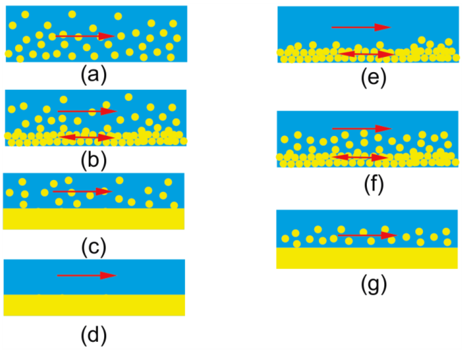
The transient cuttings transport modeling approach is required to capture the details of the unevenly distributed cuttings bed during practical drilling. This study employs a generalized transient solid–liquid, two-phase flow model developed in a previous work [46] to obtain the dynamic cuttings distributions in a wellbore. In the generalized model, the flow patterns of solid–liquid mixtures are classified into several different patterns to cover all cuttings transport possible scenarios, as shown in Figure 2. The formulations of the model are based on transient mass and moment conservations, and the equations can be adjusted automatically according to the change in the flow patterns. Thus, the model can handle the change in flow patterns in both the time domain and space domain. By using this approach, the process of cuttings transport from bit to surface can be tracked continuously during the entire drilling process while considering the dynamic change in drilling operational parameters. Details of the model are shown in Appendix A.

Figure 2.
Possible cuttings flow patterns in a wellbore cited by [43]. Reproduced with permission from [46].
3. Coupling of Transient Hole Cleaning and Drill String Model
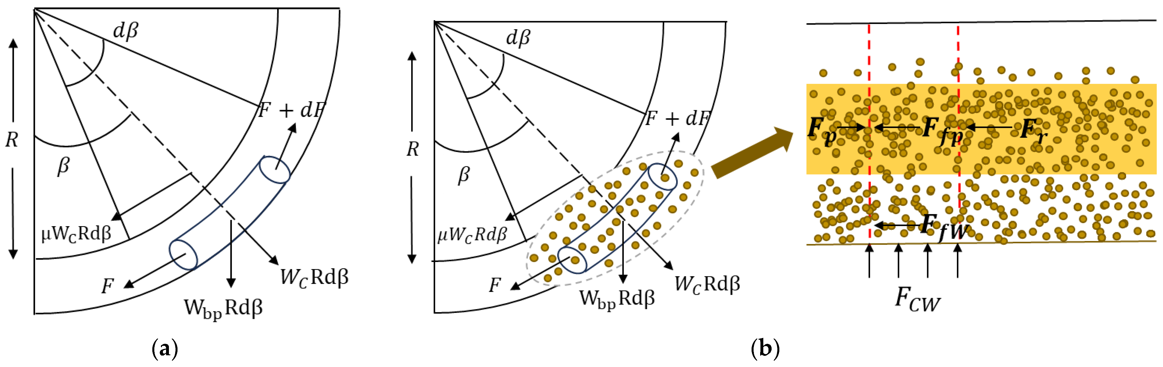
It is commonly recognized that accumulated cuttings beds in the deviated or horizontal sections of a wellbore can increase the friction force on the drill string, which leads to changes in torque and axial load. Experimental studies show that the torque on the drill string increases significantly as the cuttings bed builds up in the wellbore [46]. To consider the effect of the cuttings bed on the forces along the drill string, a new torque and drag model is proposed by modifying the traditional soft string model. The effect of the cuttings bed on the drill string can be illustrated by using Figure 3. For a given section of the drill string, the traditional approach to obtain the axial force (as shown by Ft in Figure 4) is shown in Figure 3a, where Wc is the unit contact force, Wbp is the unit buoyant weight, R is the radius of curvature, and β is the rotation angle. To simulate the influence of accumulated cuttings, an additional frictional force (Ffw) was added at the location of the cuttings bed, which is related to the contact force (Fcw) between the cuttings bed and the wellbore, the friction coefficient (fws) between the cuttings bed and the drill string, and the depth of the drill string. The detailed calculation method for this additional force is shown in Figure 3b. In addition, in the figure, Fp is the axial force at the lower end of the elemental section, Ffp is the axial force exerted by the drilling fluid on the elemental section, and Fr is the axial force of the elemental section. To model the exact effect of the cuttings bed on the drill string, detailed positions of the drill string are required for the entire wellbore, which needs complicated finite element simulations to be conducted. For practical applications, we propose to use one term to represent the complex interactions between the cuttings bed and the drill string in the soft string model, which can be estimated by using experimental data.
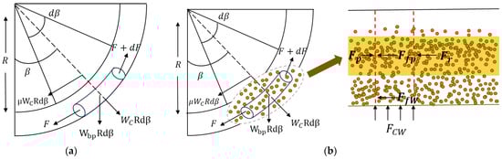
Figure 3.
Effect of the cuttings bed on the free body diagram of a drill string element. (a) Free body diagram of a drill element without a cuttings bed. (b) Free body diagram of a drill element with a cuttings bed.
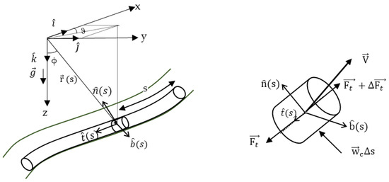
Figure 4.
Free body diagram for a drill string element in a 3D wellbore cited by [25]. Reproduced with permission from [27].
The newly proposed model follows the assumptions of the traditional soft string model, as follows:
- The drill string is considered as a soft string, and the bending stiffness is neglected;
- The drill string is in continuous contact with the wellbore.
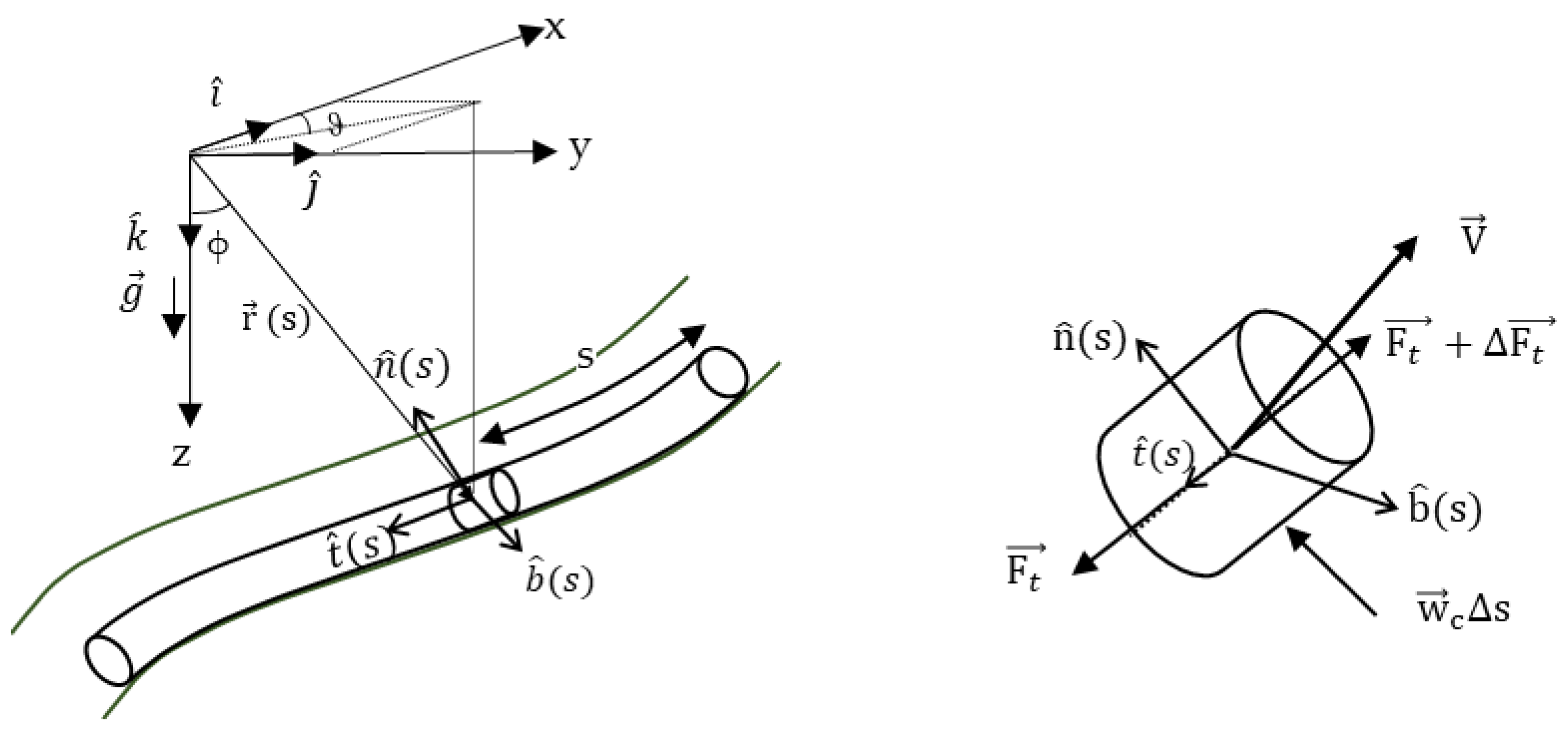
For the sake of simplicity, the commonly used Cartesian coordinates with unit vectors are transformed into the Frenet–Serret coordinates with unit vectors , as shown in Figure 4. The relation between the direction cosines of Cartesian and Frenet–Serret coordinate systems is represented by Equations (1)–(3).
where φ is the inclination angle and ϑ is the azimuth angle.
Starting from the free body diagram of one drill string element and following a similar approach as in existing works [19,49], the force and moment equilibrium equations for a rotating drill string can be obtained. The modifications are the additional forces from the cuttings bed, as shown in Equations (4)–(8). For example, for the cases of tripping in, the additional resistance force Fcb is applied opposite to the axial direction to represent the effect of the cuttings bed on the axial force. For a rotating drill string, the additional resistance force Fcb would be tangential to the drill string wall curve and pointing in the opposite direction of the rotating direction.
where Ft is force in the tangent direction (axial force); wbp is the unit weight of the drill string; wc is the contact force; nz and bz are the normal and binomial Frenet–Serret unit vectors in the z direction, respectively; θ is the direction of the normal contact force component in the plane; Fcb is the additional force caused by the cuttings bed; is the pipe curvature; is the friction coefficient; and is the magnitude of moment (torque) required for pipe rotation, the product of the tangential force, friction coefficient , and rotation radius, where the tangential force direction aligns with the tangent of the drill string’s motion.
The unit contact force and θ can be obtained by Equations (9) and (10).
The algorithm to solve the modified soft string model is similar to the standard torque and drag model, except that at each element, the additional resistance force Fcb needs to be calculated based on the local cuttings bed height.
The dynamic hole cleaning model discussed in the previous section is run by taking the drilling operational parameters as inputs and predicts the dynamic cuttings bed distribution along the wellbore. The modified soft string model takes the predicted cuttings bed distribution results as inputs, then calculates the local Fcb at each discretized point, and at last solves for the torque and drag along the string. A key point in this approach is obtaining the relation between Fcb and the cuttings bed height, which is discussed in the following experimental investigation section.
4. Experimental Investigation of Effect of Cuttings on Drill String
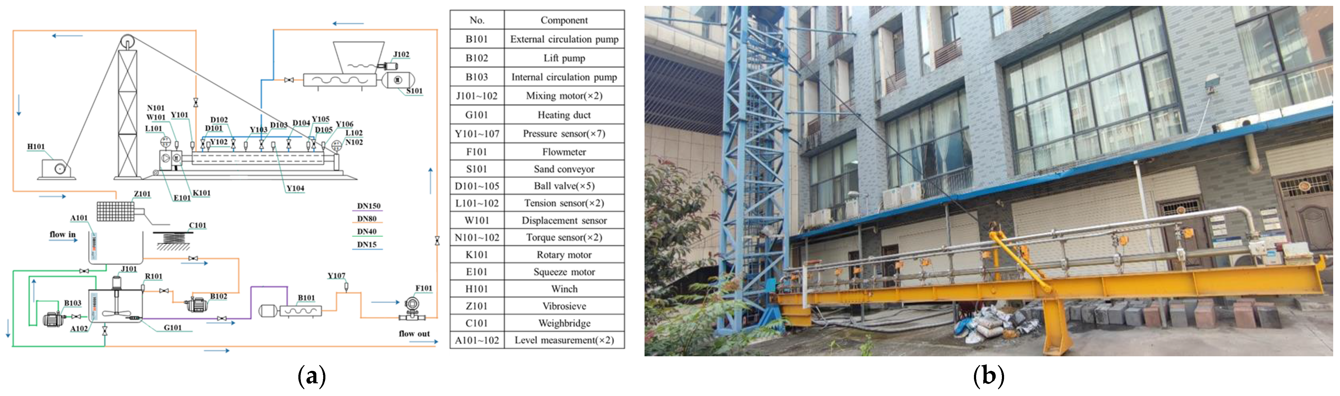
The Wellbore Flow and Intelligent Drilling Test (WFIDT) facility at Yangtze University was used to conduct experimental tests on the effects of cuttings on the force acting on the drill string. Graphical information of the facility is shown in Figure 5. It contains an annulus test section, a circulation and solid handling module, a hoisting module, a pipe rotating and axial moving module, and a data collection and control module. The test section is composed of a transparent outer pipe to simulate the wellbore and a metal inner pipe to simulate the drill string. The transparent outer pipe allows observation of the height of the cuttings bed and the friction testing process. The length of the test sections is 15 m, and there are several size combinations for the annulus geometry, which include 88.9 × 139.7 mm, 50.8 × 101.6 mm, and 25.4 × 50.8 mm. Driven by two different motors, the inner pipe can rotate and move in the axial direction inside the wellbore. The maximum rotation speed is 150 RPM, and the maximum moving distance is 20 mm (compressed or stretched in the axial direction by the axial motor). The torque and axial forces on the drill string can be recorded by using the sensors arranged at both ends of the drill string during a test. The inclination angle of the test section can vary between horizontal and vertical by using a hoisting system. The circulation and solid handling module include a mud pump, a solid injection system that injects cuttings into a fluid flow, and a solid collection system that separates the cuttings from the fluid. During a test, the cuttings movement and fluid flow can be directly observed from the test section. Pressure and temperature data can be obtained from a number of sensors distributed along the test section.

Figure 5.
Experimental facility: (a) schematic of facility; (b) overview of facility.
A test to investigate effect of cuttings on the drill string include the following steps: (i) start the system and circulate the system with pure drilling fluid to clean the wellbore and flow lines; (ii) rotate the drill string at a desired speed and record the steady torque values at both ends; (iii) stop the rotation, move the drill string in the axial direction, and record the axial load at both ends; (iv) inject cuttings into the system and conduct a normal cuttings transport test until the cuttings distribution reaches steady state; (v) record the cuttings bed height; (vi) rotate the drill string at a desired speed with cuttings in the wellbore and record the steady torque value at both ends; (vii) stop rotation, move the drill string in the axial direction with cuttings in the wellbore, and record the axial load at both ends; and (viii) flush the system. Six parameters are measured from a test, which include the torque value during rotation without cuttings, axial load during axial motion without cuttings, cuttings bed height, pressure drop, torque value during rotation with cuttings, and axial load during axial motion with cuttings. The same experimental procedure is carried out under different conditions of the cuttings bed height. Each experiment is repeated three times to improve the accuracy of the test results. The experiment is conducted at room temperature and atmospheric pressure.
In addition to the newly conducted tests results, existing data from the literature were also used in the analysis [21,54,58,59]. The matrix for all available data used to develop the correlations in the sections is shown in Table 1. All data were obtained from tests conducted using water-based drilling fluids, where the behavior index is 0.814, and the consistency index is 0.065 pa·sn. Quartz sand was used as the cuttings, with a density of 2667 kg/m3 and a particle size range of 2–5.66 mm.

Table 1.
Test matrix for the analyzed data.
The changes in torque and axial load for conditions with and without cuttings under the same test conditions are analyzed, which were used to develop correlations in the following sections.
4.1. Effect of Cuttings Bed on Torque
For the purpose of convenience, the cuttings bed height and its effect on torque are normalized by using Equations (11) and (12), respectively.
where hbed is the cuttings bed height, Dw is the well diameter, is the normalized bed height, is the measured torque value at the corresponding normalized cuttings bed height , Tclean is the torque value without cuttings for the corresponding wellbore configurations, and TCR is the torque change ratio, which is caused by the cuttings bed. After normalization, the relationship between the dimensionless bed height and the torque change ratio TCR is shown in Figure 6.
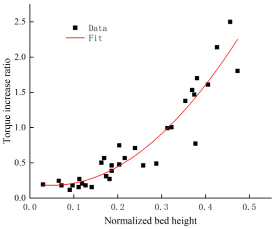
Figure 6.
Plot of normalized bed height and torque change ratio.
From Figure 6, it can be seen that the relationship between the normalized bed height and the torque change ratio roughly follows an exponential function. Thus, an exponential function correlation is developed based on the data set, which can be expressed by Equation (13).
where α = 20 and β = 2.5 are two constants.
Because the tests were conducted in facilities that simulate a part of a straight hole, the torque value is proportional to two factors: the contact force between the wellbore and the drill pipe, and the friction coefficient between the wellbore and the drill pipe. For the results shown in Figure 6, the contact force remains constant throughout the tests, and the change in torque is only caused by the change in the friction coefficient. Because the parameters are dimensionless, Equation (13) can be converted to represent the relationship between the normalized bed height and the change in the additional circumferential friction coefficient caused by the cutting bed between the wellbore and the drill pipe, which is shown in Equation (14).
where κ = 6.78 and η = 0.88 are two constants. fCR is the additional circumferential friction coefficient caused by the cuttings bed, which is defined by Equation (15).
where is the friction coefficient with normalized cuttings bed height, , and is the friction coefficient without cuttings. For torque calculation in a complex well with cuttings beds, Equation (16) can be applied to the torque and drag model discussed in the previous section with the given local bed heights, which can be obtained from the transient cuttings transport model. It needs to be pointed out that is an equivalent friction coefficient change ratio that includes all the changes in the friction force caused by the cuttings bed. It is defined by using the ratio between the friction force with cuttings beds and the original contact force for no cuttings conditions. Thus, it is a representation of the changes in friction forces caused by the cuttings bed instead of the actual friction coefficient.
4.2. Effect of Cuttings Bed on Axial Friction Force
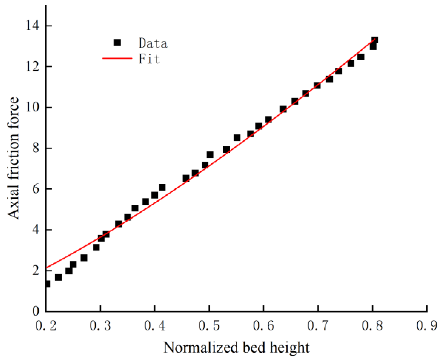
For cases where the drill string moves axially, the relationship between the axial friction force and the dimensionless bed height can be represented by a linear relationship, as shown in Figure 7, which is consistent with the findings of other researchers [60].
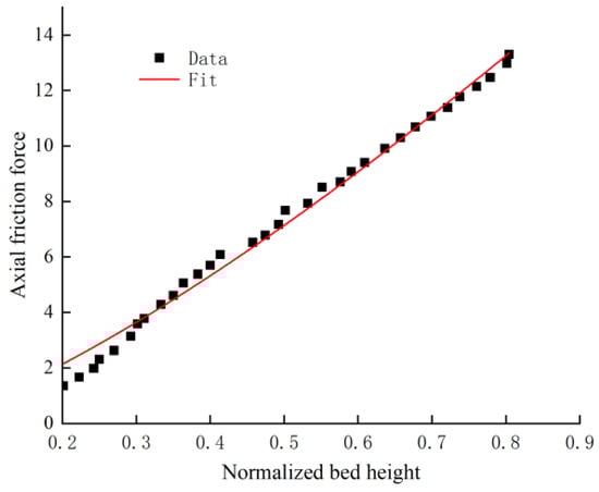
Figure 7.
Relationship between normalized bed height and axial friction force.
The additional axial friction force from the cuttings bed can be obtained using Equation (16).
where k = 20.743 and c = 3.314 are two constants.
Following the definition in Equation (15), the relationship between the dimensionless bed height and additional equivalent sliding friction coefficient caused by the cuttings bed can be expressed by Equation (17), which is applied to the drill string model discussed in the previous section to consider the effect of cuttings on the axial friction force.
where a, b are empirical coefficients. It needs to be pointed out that a number of parameters can change in practical drilling applications compared to the experimental tests. The purpose of the experimental study was to find a general formation that can be used in the modified drill string model. The correlations developed from the experimental data may not be applicable for all situations. For conditions that were not covered by the test matrix, the fitting parameters can vary significantly, but the trend should be the same. In other words, Equations (14) and (17) are still valid, but the equivalent coefficients may be different for different scenarios. More new data with new types of drilling fluids and pipes would be valuable to make the model applicable for a broader range of situations. The model can also be improved by fitting the model with field data, which was performed in the following case study, and the procedures to tune the model are listed as follows:
- Collect benchmark data for the standard drill string model, which represents the friction forces on the drill string under the no cuttings scenario (the data measured when there is little cutting accumulated in the wellbore, e.g., after a thorough circulation or wiper trip was performed). The torque benchmark data can be obtained by selecting the surface torque value under off-bottom rotations, and the axial force benchmark data can be obtained from the hookload data under tripping in or pulling out.
- Construct the object function for standard drill string model tuning to obtain the friction coefficients for the specific well under no cuttings conditions:
- 3.
- Collect tuning data for the coupled model, which represents the friction forces on the drill string with cuttings in the wellbore. The torque and axial force values can be obtained by using the same method in step 1, and the difference is that the data should be collected under conditions where there are cuttings in the wellbore. It should be noted that the data collection in this step should be conducted after a certain length of new well section was drilled after step 1, and all the operational parameters (e.g., ROP, pumping flow rate, rotation speed) should be collected to analyze the downhole cuttings distributions, which is discussed in the next step.
- 4.
- Run the transient hole cleaning model by using the operational data collected in step 3 as inputs, and estimate the downhole cuttings distribution for the given condition.
- 5.
- Repeat steps 3 and 4 several times to obtain multiple data points for regression.
- 6.
- Construct the object function for hole cleaning coupled drill string model tuning to obtain the friction coefficients:
- 7.
- Solve the objective functions in steps 2 and 6 by using proper optimization algorithms.
5. Case Study
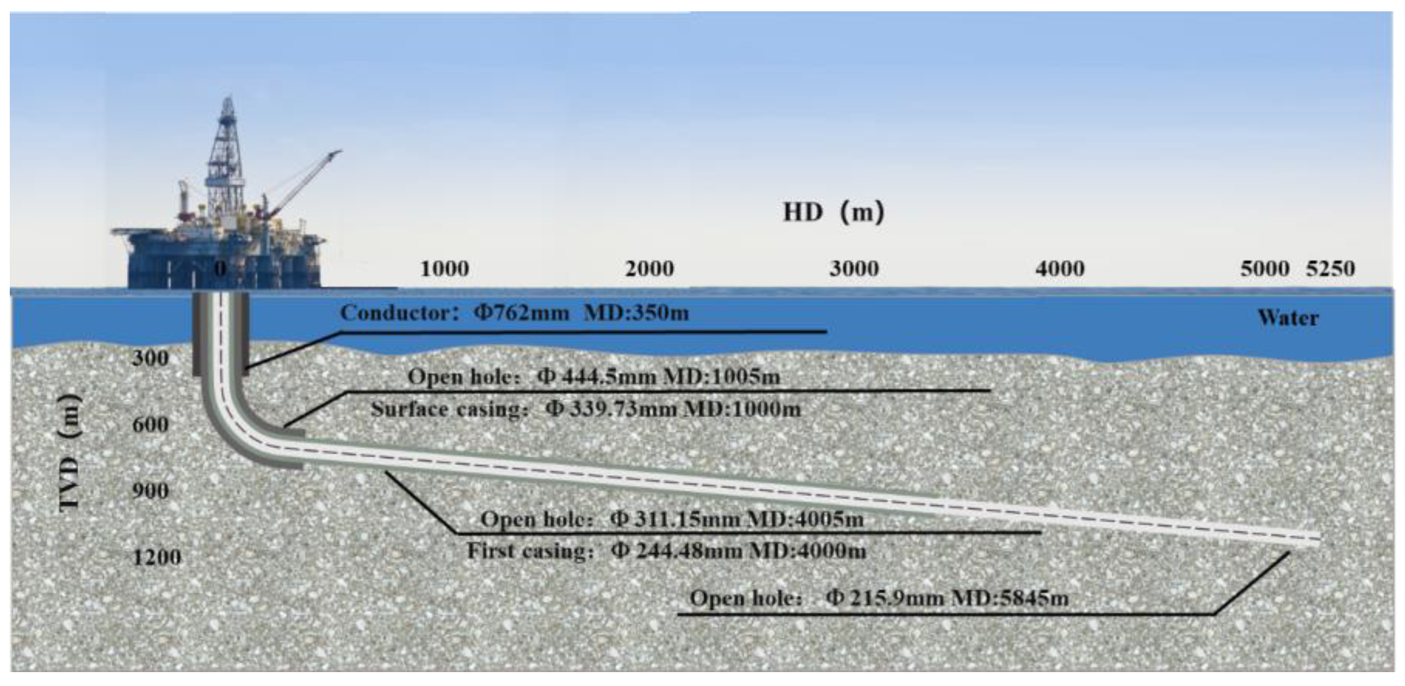
In this section, the model developed in the previous sections is applied to practical drilling activities to demonstrate the effects of the dynamic cuttings distribution on the drill string. The well information for case analysis is shown in Figure 8. In this example, the kick-off depth is about 400 m, and the inclination angle reaches 85° at about 900 m and is kept constant thereafter up to 5845 m. The azimuth remains unchanged at 112.35°. The ratio of the horizontal displacement to the true vertical depth (HD/TVD) is 4.27. The bottom hole assembly (BHA) components are listed in Table 2, and the drilling fluid information is shown in Table 3.
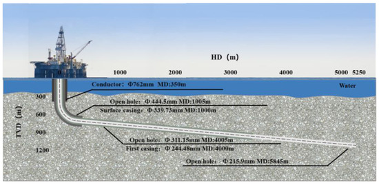
Figure 8.
Schematic of the case study well.
Table 2.
BHA components.
Table 3.
Fluid Properties.
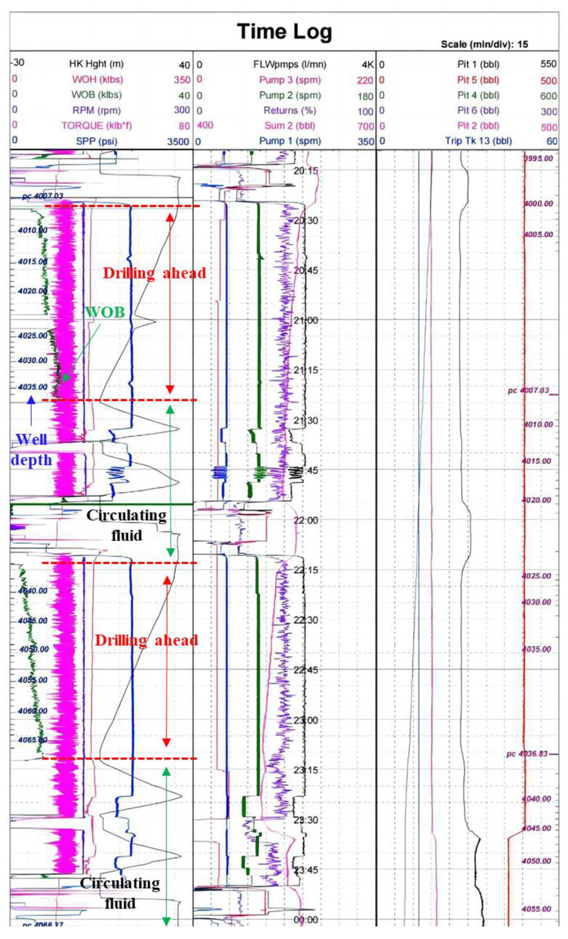
The rate of penetration (ROP) during the drilling process was 40 m/h, and the well was circulated for about 45 min after each stand was drilled. The operational parameters during a typical drilling cycle are shown in Figure 9. In this case study, we investigated the period during drilling the sections between ~4000 and 4200 m MD. It is assumed that the borehole has been completely cleaned before drilling this section because it is the start of the 215.9 mm wellbore section, which follows the 244.48 mm casing. It needs to be pointed out that the model was tuned to match the field measurements by adjusting the coefficients in the correlations for the friction factor, and details can be found in a previously published paper. The purpose of this case study was to demonstrate the value of the coupled model in practical drilling instead of validating the correlations developed in the previous section.
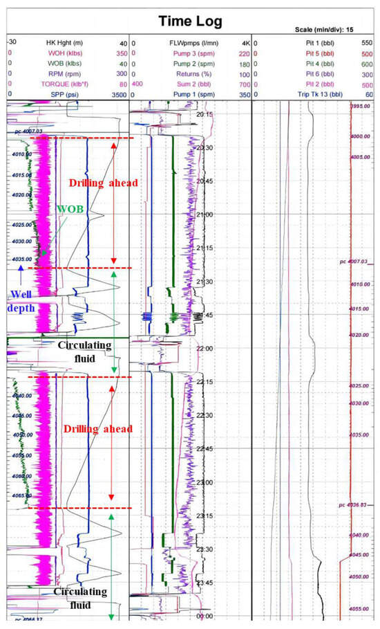
Figure 9.
Field data of a typical drilling process.
5.1. Dynamic Hole Cleaning Results
Before drilling the new wellbore section, there were no cuttings in the wellbore because a new casing was set in place. As the bit moved forward to drill the new formation, cuttings were generated and transported towards the wellhead from the bottom hole. Because of the alteration between penetration and circulation (the wellbore was cleaned by circulating with one bottom up (BU) after each stand was drilled), new drilled cuttings were feed into the annulus from the bit periodically. Therefore, the distribution of cuttings in the wellbore followed a wavy pattern, as shown in Figure 10. This figure shows the cuttings concentration along the entire wellbore at 45 min, 135 min, 225 min, 315 min, 405 min, and 495 min after the start of drilling the new section at 4000 m MD. These six time points represent the completion of drilling the first, second, third, fourth, fifth, and sixth stands, respectively.
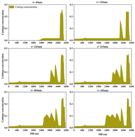
Figure 10.
Dynamic distribution of cuttings concentrations along wellbore.
At t = 45 min, the first cuttings bed wave was generated by cuttings from drilling the first stand. At this time, the cuttings bed was between ~3700 and 4000 m MD, and the maximum cuttings concentration was around 23% (equivalent to 80 mm cuttings bed height) in this section of the wellbore. There was a small amount of cuttings ahead of the cuttings bed wave, which were the cuttings suspended in the drilling fluid because the suspended cuttings traveled much faster than the cuttings bed. During circulation after drilling the first stand, the cuttings bed wave was pushed upward and eroded. Another cuttings bed wave was generated during drilling the second stand and then flushed upward once the penetration process was interrupted, as shown in Figure 10 at t = 135 min. Similarly, a cuttings bed wave was generated during drilling each of the following stands. As the cuttings bed waves were flushed towards the wellhead, the height of the waves diminished because the rate of cuttings feed into a specific wave (mainly from the cuttings in suspension mode) was less than the cuttings generation rate at the drill bit. The cuttings bed waves moved in the wellbore in a way similar to the motion of sand dunes in a desert. Particles were picked up at the upwind direction and deposited back at the other end of the dune. The moving speed of the cuttings bed waves decreased as their height decreased because the in situ flow velocity decreased. Thus, the newly generated waves could catch up with the older waves after a certain amount of time and formed a longer cuttings bed. Therefore, significant amounts of cuttings were accumulated in the wellbore after drilling for a long period of time, as shown at t = 495 min in Figure 10.
The reason for the accumulation of cuttings was that the deposited cuttings bed was not fully cleaned out of the wellbore during the circulation periods, either because the flow rate was not high enough or the circulation time was not long enough.
From a practical point of view, the flow rate used during drilling was constrained by a number of factors. However, to clean the well efficiently, the flow rate should be no less than the minimum required flow rate to suspend and transport the deposited cuttings when ROP is zero. In this scenario, increasing the circulation time became a practical choice to clean the well. One of the most important engineering problems during drilling long lateral wells is to optimize the circulation time, circulation frequency, and ROP. The constraints for the optimization include the effect of the cuttings bed on the ECD and the drill string, which are discussed in the following sections.
5.2. Effect of Dynamic Cuttings Distribution on ECD
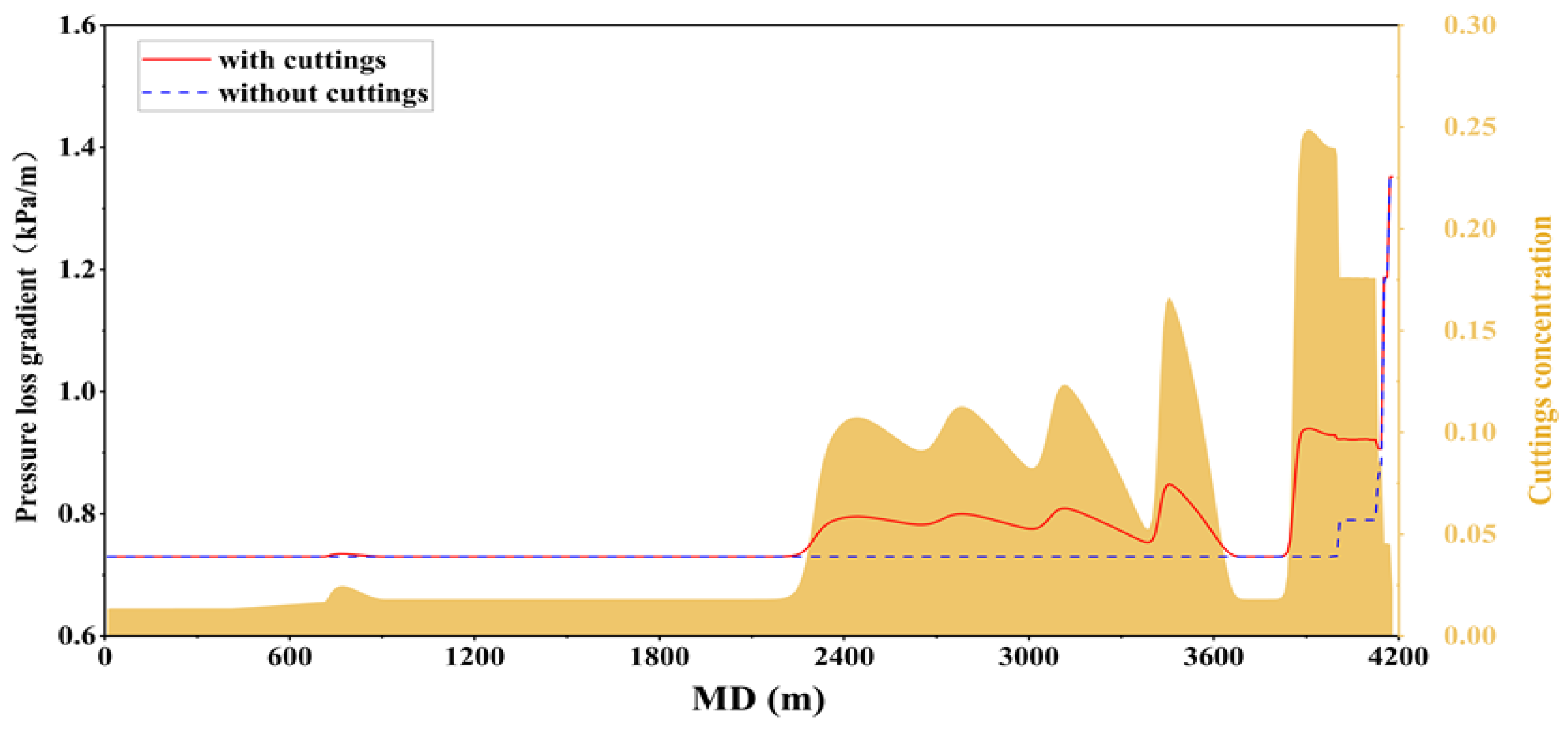
It is generally accepted that cuttings can change the flow pressure loss in the annulus significantly, and details can be found in a previous study [54]. In ERD drilling, one of the constraints is that the ECD should not exceed the safe mud weight window. In practical drilling, the ECD increases as the horizontal lateral increases, while the safe mud weight window stays almost constant. There are two factors that contribute to the increase in ECD: the increase in well length and the cuttings. The transient cuttings transport model employed in this study can simulate both dynamic cuttings distributions (as shown in Figure 10) and the detailed effects of cuttings on the annulus pressure loss, as shown in Figure 11. It needs to be pointed out that to highlight the pressure changes caused by circulation and cuttings, the static pressure caused by the pure drilling fluid was eliminated from the overall pressure gradient.
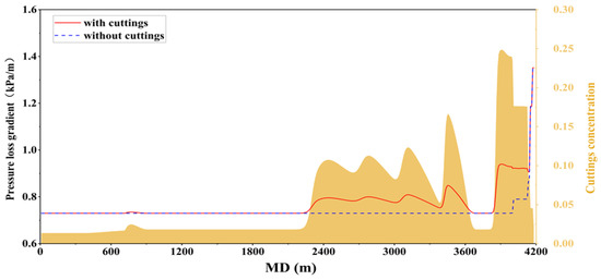
Figure 11.
Effect of cuttings on wellbore pressure at t = 495 min.
By comparing the wellbore pressure gradient with and without considering the effect of cuttings in Figure 11 (the red solid line and blue dashed line), it can be seen that unevenly distributed cuttings in the horizontal lateral caused important changes in the pressure gradient. If there were no cuttings in the wellbore, the pressure gradient should be constant. At the locations with cuttings beds or dunes, the actual pressure gradients with cuttings considered increased accordingly. The cuttings-induced pressure loss led to significant changes in the ECD, as shown in Figure 12.
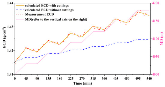
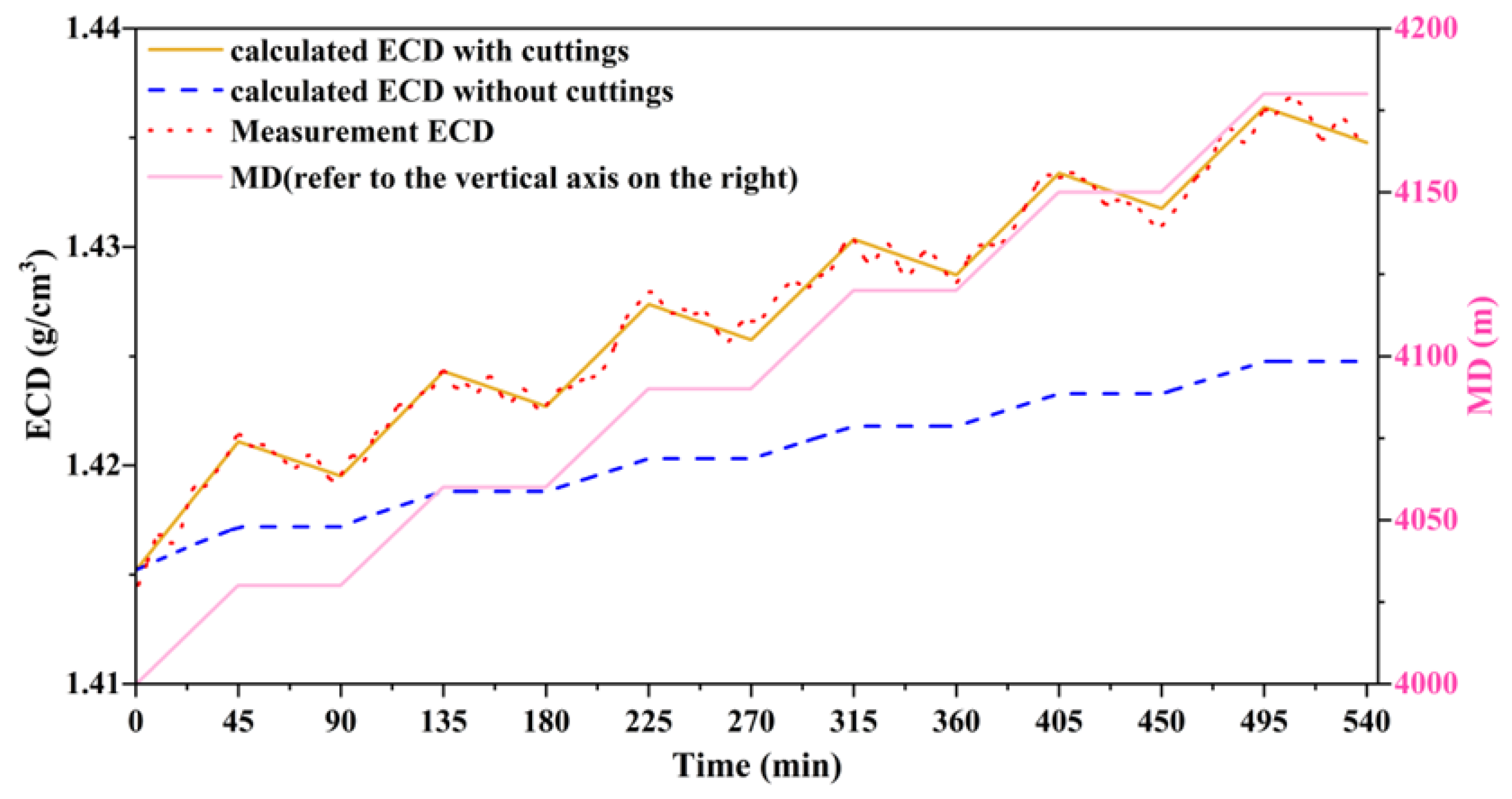
Figure 12.
Dynamic changes in the ECD during the analyzed time period.
Figure 12 illustrates the changes in the ECD during the period of drilling the six stands. The yellow line and the blue line represent the ECD with and without considering the effects of cuttings, respectively. The red dots are the measured ECD from field data. The pink line represents the changes in the well measured depth (MD), which refers to the vertical axis on the right side of the figure. As the well depth increased, the two ECD values increased at different rates. The effect of the ECD considering cuttings increased faster than the ECD without considering cuttings. During the circulation periods (the time periods when the well depth was constant), the effect of the ECD without considering cuttings was kept constant, and the ECD with cuttings considered decreased as new cuttings generation stopped and the cuttings were transported out of the wellbore. If the circulation was sufficient and all the accumulated cuttings were cleaned away, the yellow line would decrease to the same value as the blue line. As more stands were being drilled, the difference between these two ECD values increased because the amount of cuttings accumulated in the wellbore increased. The results in Figure 12 are helpful to practical drilling applications in two ways: (i) they could be used to monitor the actual wellbore pressure and keep it within the safe window (especially in narrow mud weight window conditions), and (ii) they could be used to guide the circulation time and frequency to ensure the cuttings inside the wellbore are not imperiling normal drilling from the ECD perspective.
5.3. Effect of Dynamic Cuttings Distribution on Drill String
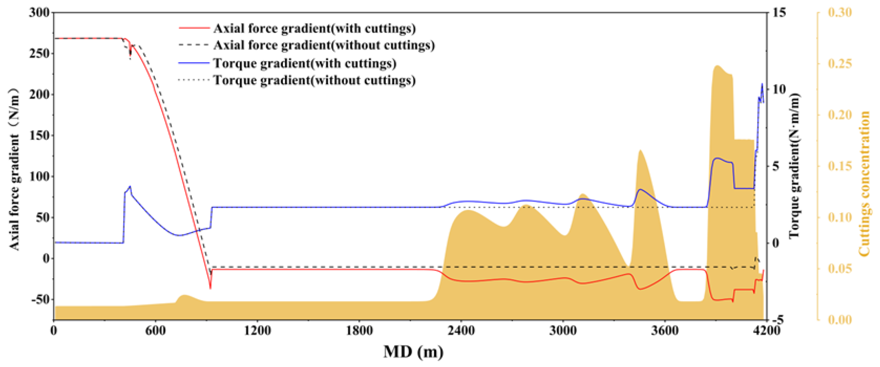
As discussed in previous sections, another important factor that limits long lateral drilling are the friction forces on the drill string (including the torque and axial force), which are also closely related to cuttings distributions. The torque and axial force gradients along the drill string during the penetration process at t = 495 min are shown in Figure 13. In the shallow parts of the well (MD < 2000 m), the effects of cuttings on the drill string were negligible because the cuttings concentrations were low and mainly suspended in drilling fluids. In the well sections with deposited cuttings beds, the friction forces on the drill string increased proportionally with the cuttings concentration compared to the no cuttings scenario, which was reflected in the differences between the axial force gradients and torque gradients for conditions with and without considering cuttings effects. As discussed in the previous sections, the reasons for increasing the friction forces as the cuttings concentration increases mainly include two aspects: (i) the averaged friction coefficients caused by the cuttings bed around the drill pipe increase because the contact area between the pipe and cuttings bed increases; and (ii) the cuttings bed constrains the movement of the drill string and adds additional contact forces, e.g., part of the cuttings bed’s weight is borne by the drill string.
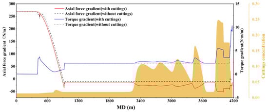
Figure 13.
Effects of cuttings on gradients of forces on drill string.
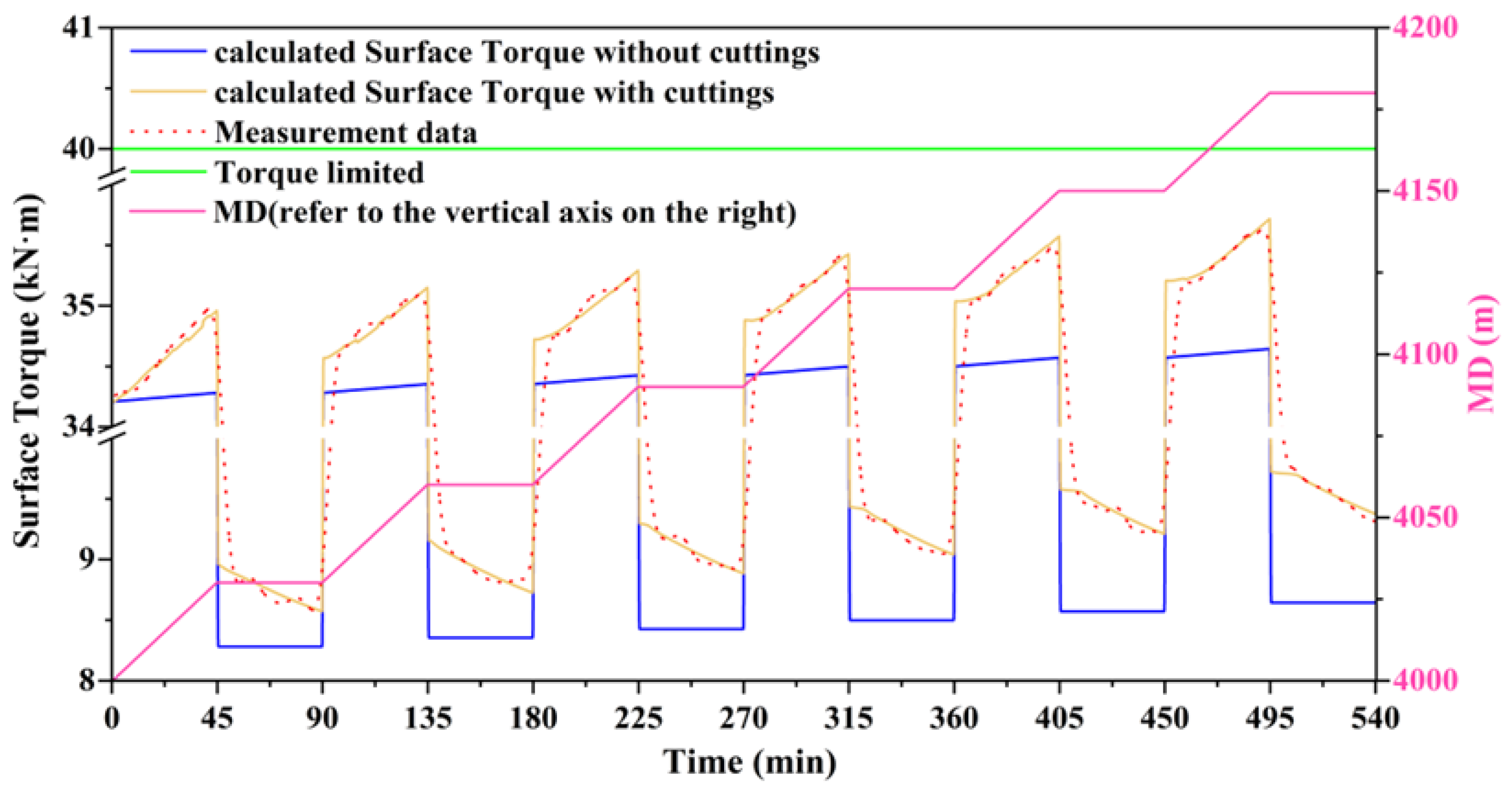
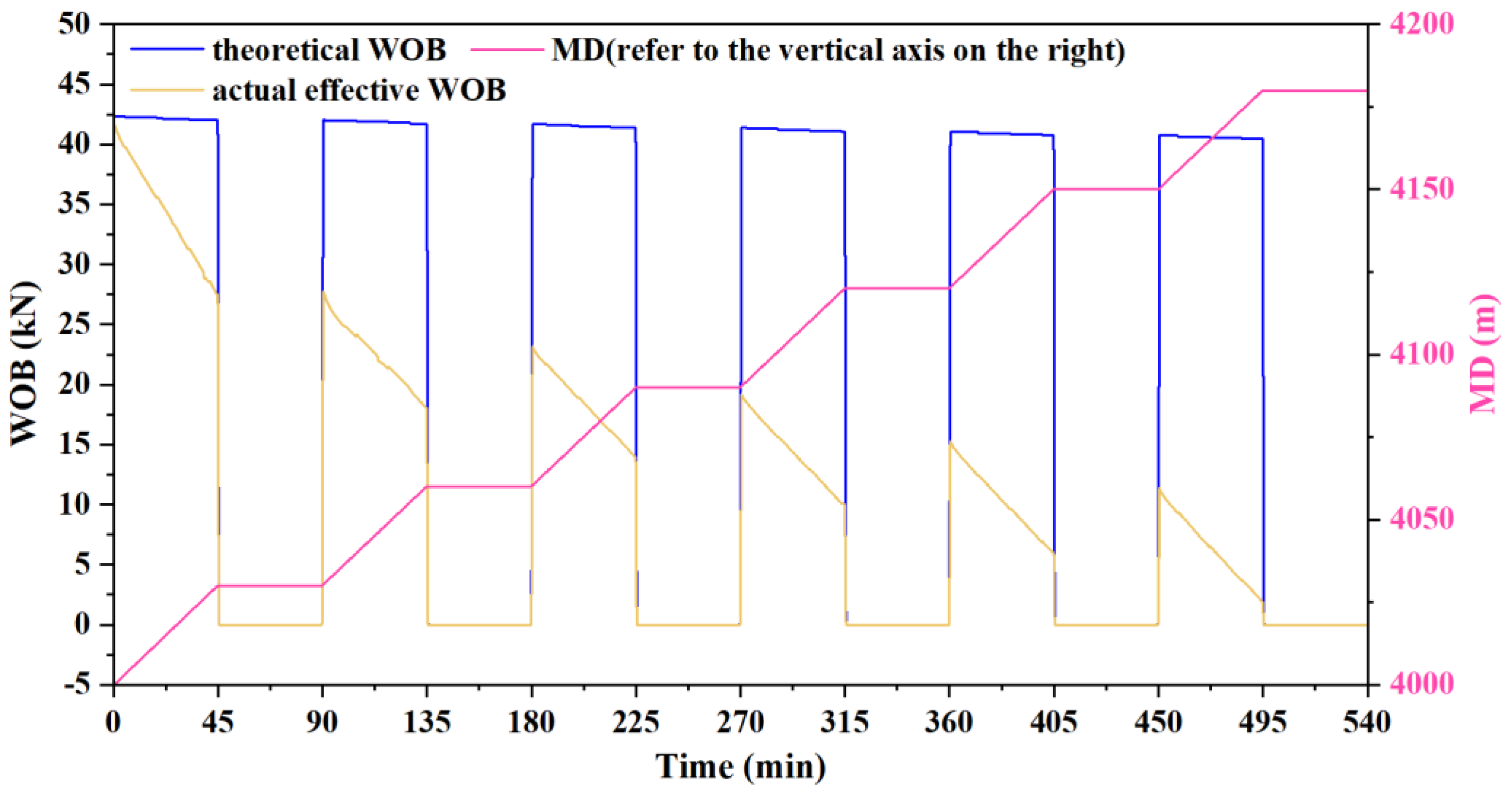
In practical drilling applications, one straightforward way to reflect and monitor forces on the drill string is to use surface torque and actual WOB during penetration. High torque could lead to severe damage to the drill string or stuck pipe incidents, and low WOB could lead to a decrease in the ROP. The changes in surface torque and WOB during the drilling of the six stands are shown in Figure 14. As shown in Figure 14, if cuttings were not considered, the surface torque increased slightly during the penetration process (because the well depth increased) and remained constant during the circulation process (the sharp changes between circulation and penetration were the torque from the drill bit, which can be neglected during circulation because the bit was off bottom). For conditions where the effect of cuttings was considered, the surface torque increased significantly during the penetration process as the cuttings accumulated in the wellbore. During the following circulation process, the surface torque decreased as the cuttings were removed out of the wellbore, which was consistent with the field data. The difference between the initial surface torque values at the beginning of drilling each stand for scenarios with and without considering cuttings grew larger as the well went deeper. This was another indication that the wellbore was not circulated enough to remove all the accumulated cuttings. From this figure, it can be seen that the increase in surface torque caused by cuttings was significant, and the upper limit for surface torque could be reached much earlier than in ideal scenarios where there was no cuttings accumulation.
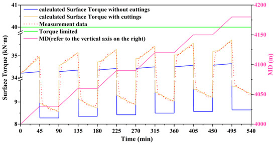
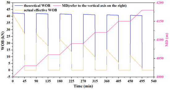
Figure 14.
Changes in surface torque and WOB during the analyzed period.
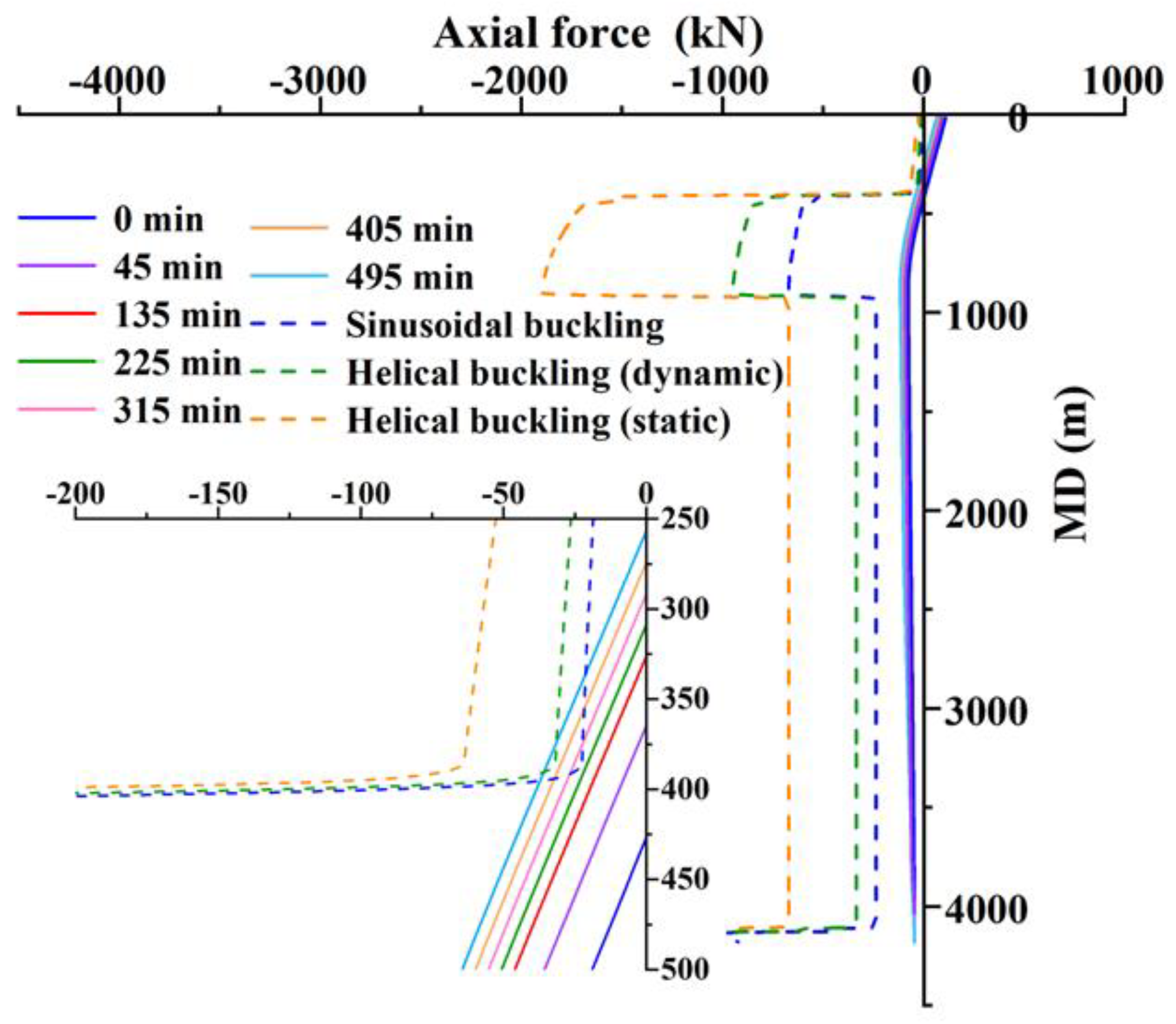
Another commonly encountered obstacle during drilling long lateral wells is insufficient WOB, which is also closely related to dynamic cuttings distributions. Figure 14 also shows the simulation of WOB by assuming that the hook load applied at the surface was constant. If there were no cuttings in the wellbore, the theoretical WOB would decrease slightly as the well depth increased, and it should not decrease significantly after drilling the six stands. However, insufficient WOB and low ROP problems were reported during actual drilling, which can be explained by the results for the scenario with considering the effect of cuttings on the drill string. With the same initial WOB at the beginning (t = 0 min), the actual WOB that considers the effect of cuttings decreased significantly after each stand was drilled. Although some recovery was gained after circulation, it was significantly smaller than the theoretical value. The difference grew as the well depth increased because more cuttings accumulated in the wellbore.
For the insufficient WOB problem, one straightforward solution is to apply more weight on the drill string. If we kept the actual WOB the same as the initial value (42.5 kN) during the drilling of the six stands, the axial force along the entire drill string could be represented by Figure 15. Because more weight was applied to compensate for the friction loss caused by cuttings, the neutral points moved upward as the well depth increased and the drill string became closer to the buckling criteria. As shown in the small embedded graph within Figure 15, within the depth interval of 350 m to 400 m in the wellbore, the green curve exceeds the critical limit for sinusoidal buckling, while the blue curve surpasses the critical limit for helical buckling. Sinusoidal buckling could occur at 225 min (three stands were drilled), and helical buckling could occur at 495 min (six stands were drilled).
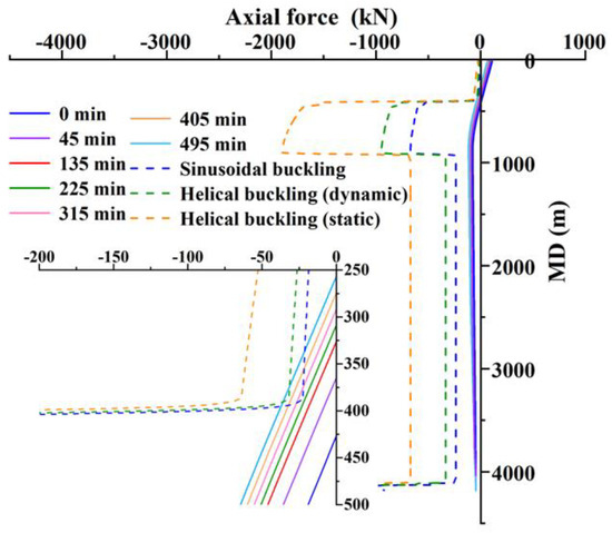
Figure 15.
Changes in axial forces during penetration process.
Therefore, the cuttings dynamic distribution could impact the friction forces on the drill string significantly, which leads to an increase in torque, a decrease in WOB, and an increase in buckling risk. Similar to the effect of cuttings on the ECD, these problems can be avoided or delayed if the cuttings in the wellbore are managed properly by optimizing the drilling parameters. In the following section, a parameter optimization method is demonstrated by using the proposed coupled model.
5.4. Drilling Parameter Optimization
In the following case, we looked into four parameters that can be easily changed during practical drilling (mean fluid velocity (equivalent to the pumping flow rate), ROP, circulation time, and circulation frequency) and converted it into a constrained optimization problem.
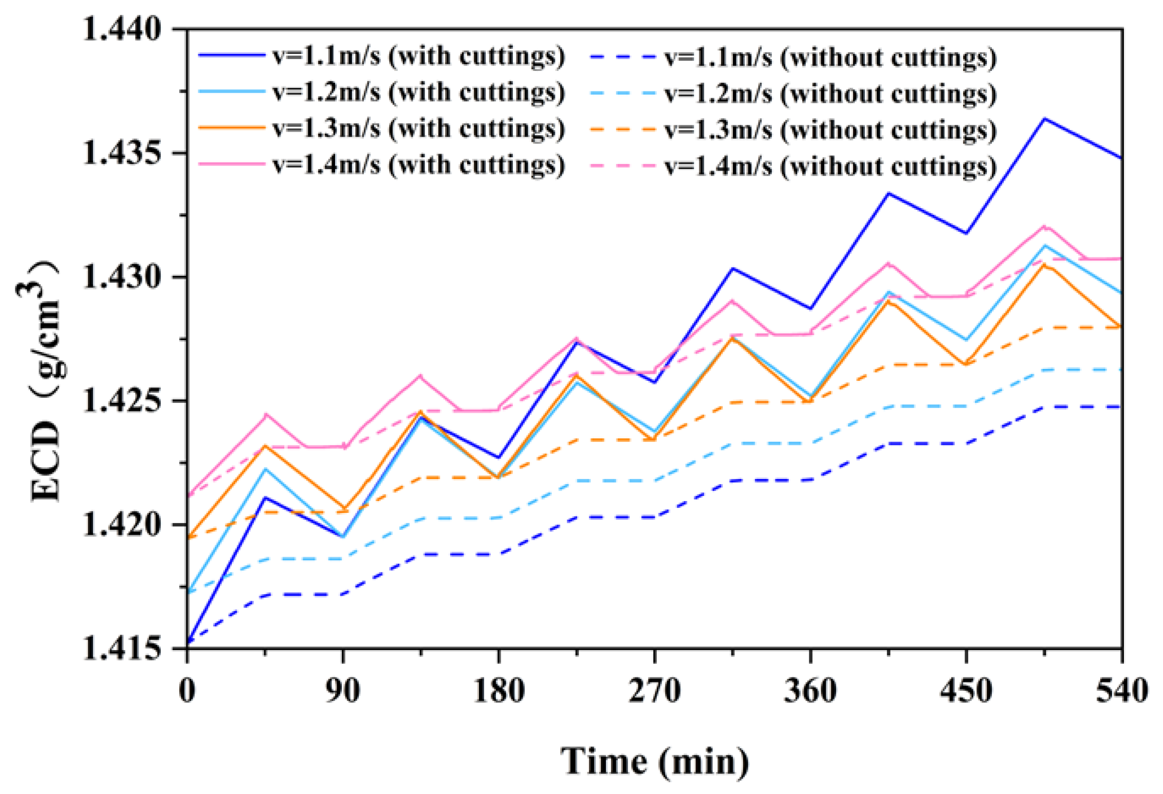
Different mean drilling fluid velocities were applied to the case discussed in the previous section (stopping drilling and circulating for 45 min after drilling each stand), and the dynamic ECD results are shown in Figure 16 (all other parameters were unchanged). From this figure, it can be seen that the ECD for pure drilling fluid flow increased as the mean drilling fluid velocity increased. However, the relationship between the velocity and ECD for the scenarios considering the effects of cuttings was more complicated. At low velocity (1.1 m/s), the ECD increased quickly as the well depth increased, and the slope became less steep as the velocity increased, which was opposite to the scenarios without considering cuttings. The minimum ECD value at t = 540 min (circulated 45 min after the sixth stand was drilled) was from 1.3 m/s, and the maximum value was from 1.1 m/s. The high ECD values at low velocities (1.1 and 1.2 m/s) were caused by accumulated cuttings (which indicated that hole cleaning was not sufficient at those conditions). At 1.3 m/s, 45 min of circulation was able to remove all cuttings in the wellbore (the ECD with cuttings fell back to the value of the ECD without cuttings at the end of each circulation, as shown in the figure). A further increase in velocity was no longer helpful in decreasing the ECD because the hole cleaning was sufficient beyond 1.3 m/s, and it led to an increase in the ECD at 1.4 m/s.
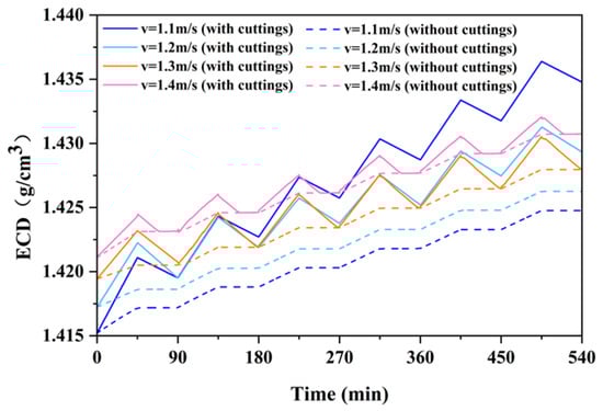
Figure 16.
ECD changes at different mean fluid velocities.
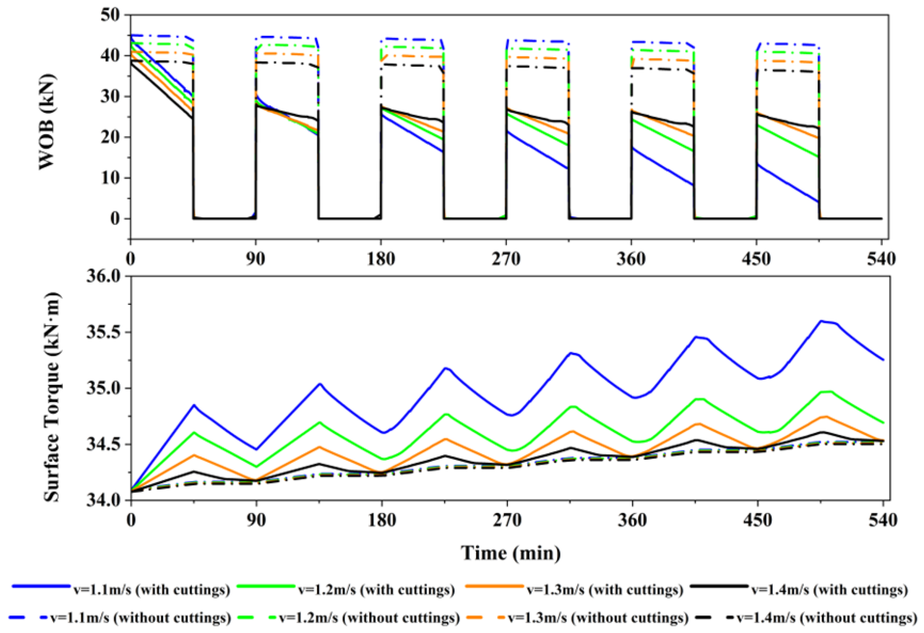
Figure 17 shows the corresponding changes in WOB and surface torque at the same operational conditions. This figure reiterates the fact that the accumulation of cuttings can significantly reduce the effective WOB and increase the surface torque for long lateral drilling. These two parameters can recover to minimum values (values that did not consider the effect of cuttings) with sufficient circulation, and the corresponding minimum mean fluid velocity was 1.3 m/s. From the results in Figure 16 and Figure 17, it can be seen that the key point to avoid ECD- and drill string-related problems during long lateral drilling is to ensure sufficient hole cleaning.
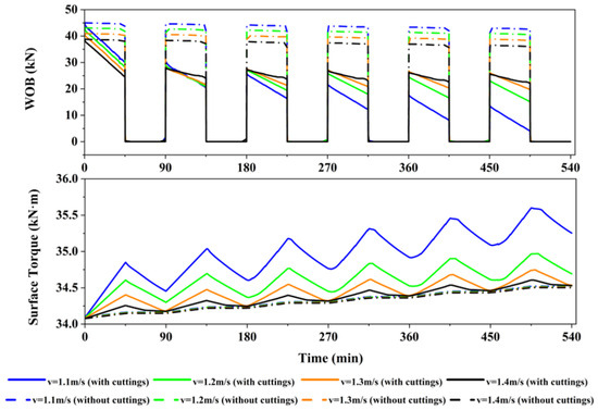
Figure 17.
Surface torque and WOB at different mean fluid velocities.
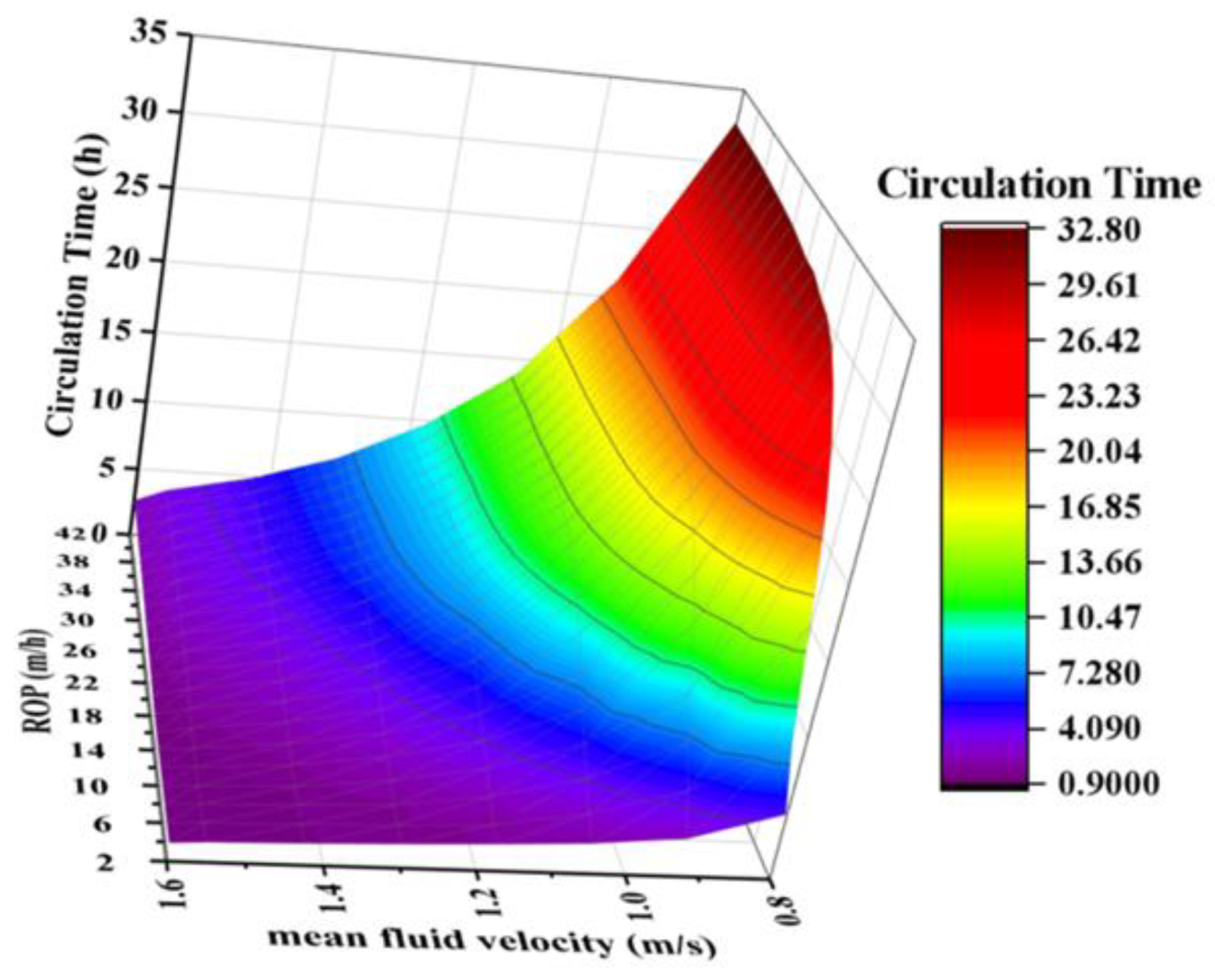
Figure 16 and Figure 17 indicate that sufficient circulation (which means the removal of all accumulated cuttings during drilling the previous stand) is a critical point to avoid the escalation of ECD- and drill string-related problems, and it can be improved by using a sufficient flow rate (which is equivalent to the mean fluid velocity). In practical drilling applications, the pumping flow rate is constrained by equipment or wellbore formation conditions. In these scenarios, a similar outcome can be achieved by adjusting the ROP or circulation time. Figure 18 shows the minimum circulation time required to remove all cuttings in the wellbore after drilling one stand at different ROP and mean drilling fluid velocities. The first step of the optimization is to determine the maximum possible mean fluid velocity. Assuming that the objective of the optimization is to minimize the overall drilling time (which is a function of the ROP and circulation time), the optimized parameters can be obtained by minimizing Equation (20) in a constrained 2D domain defined by Figure 18, where lw is the length of the well lateral to be drilled, is the length of each stand, and CT is the minimum circulation time.

Figure 18.
Minimum circulation time for different ROP and mean fluid velocities.
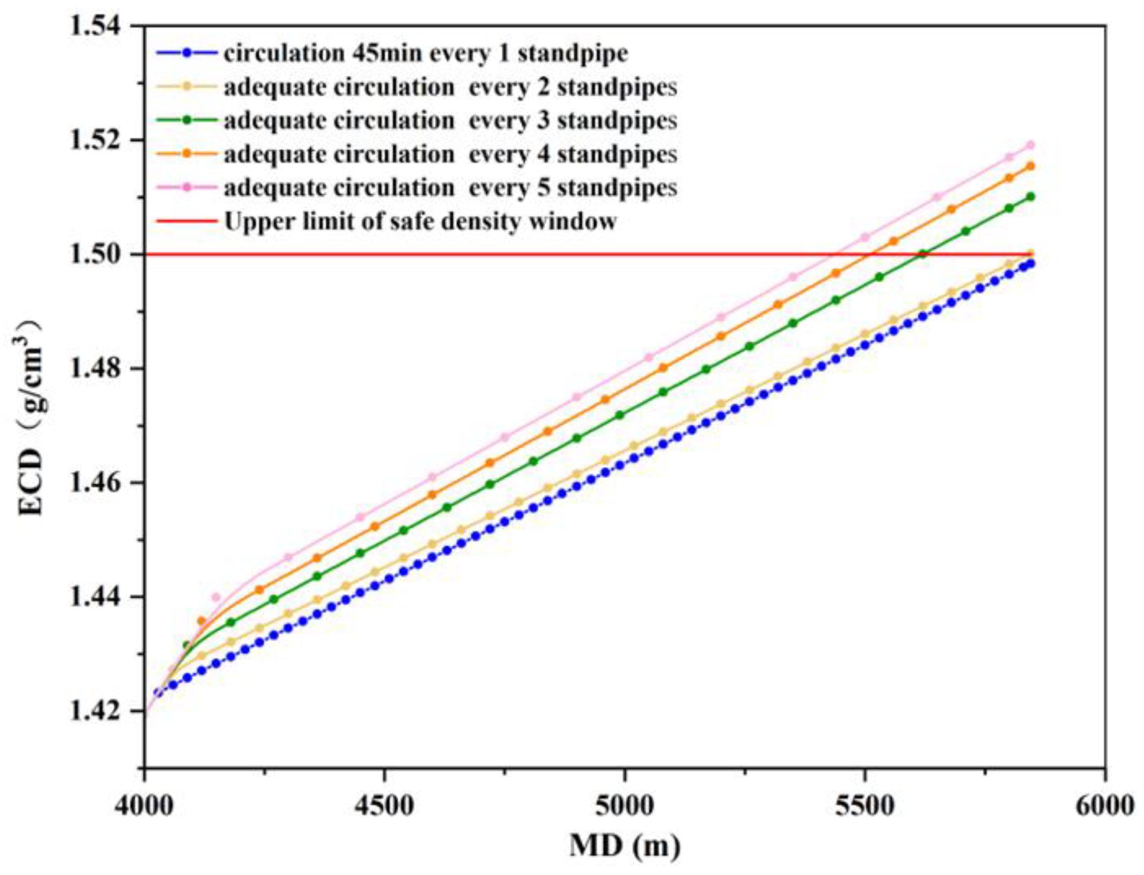
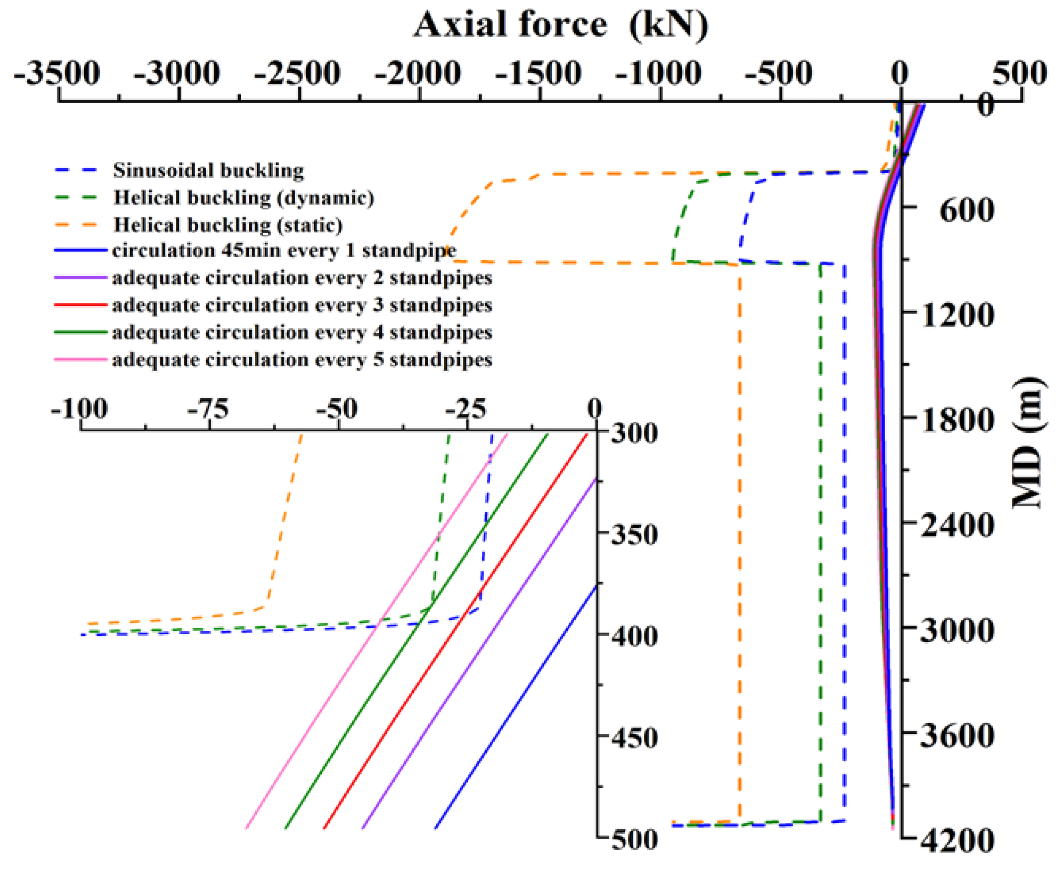
Another factor that can be adjusted is the circulation frequency, or the number of stands that can be drilled without stopping for circulation. Figure 19 and Figure 20 illustrate the maximum possible ECD and worst case drill string axial force distributions for different scenarios, respectively. Figure 19 indicates that the maximum ECD increased sharply as the circulation frequency decreased, and Figure 20 indicates that the drill string became more likely to buckle as the number of consecutive stands drilled increases; the position where the drill string is most likely to buckle was around 400 m MD. The number of stands that could be drilled continuously can be obtained by applying constraints from the safe mud weight window, maximum surface torque, and drill string buckling status (two stands to avoid sinusoidal buckling and four stands to avoid helical buckling in this case). Although the numbers can change based on cases and well depth, the method can be applied to other different cases, which is of significant value to practical drilling applications.
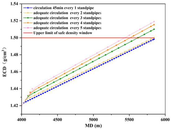
Figure 19.
ECD changes at different circulation frequencies.
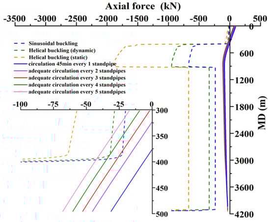
Figure 20.
Axial forces along drill string at different circulation frequencies.
6. Conclusions
(1) Through an experimental system, the influence of cuttings beds on the mechanical behavior of drill strings was investigated. It was found that the cuttings bed height significantly impacts the torque and frictional resistance: the torque increase rate exhibits exponential growth with increasing cuttings bed height, while the frictional resistance increases linearly. Based on these mechanisms, a localized correlation formula was developed to describe the relationship between the cuttings bed height and changes in drill string forces. This provides a quantitative tool for accurately evaluating the impact of cuttings beds on the torque and drag during the drilling process.
(2) By combining the localized correlation formula, transient cuttings transport model, and soft string model, a dynamic coupled model was developed to simulate the uneven distribution of cuttings beds in the wellbore and their dynamic impact on the drill string torque and drag. The simulation results show that the variations in the axial force and torque gradient are closely related to the location of cuttings accumulation. The uneven distribution of the cuttings bed leads to a more than 30% increase in the fluctuation amplitude of the drill string torque gradient.
(3) Case validation indicates that the accumulation of cuttings beds significantly affects drilling parameters. When the cuttings accumulation exceeds 25% of the wellbore cross-sectional area, the weight on bit (WOB) decreases by 281.09%, and the surface torque increases by more than 11.29%. Additionally, high cuttings accumulation leads to an increase in the equivalent circulation density (ECD), raising the risk of drill string buckling and, in severe cases, potentially causing helical buckling.
(4) In actual extended reach drilling operations, it is crucial to account for the relationship between the dynamic distribution of cuttings beds and constraints such as the ECD limit, drill string buckling risk, and surface torque limitations. Optimizing the circulation frequency or continuous drilling length is essential to ensure drilling safety. This paper proposes a novel optimization method based on the objective of minimizing the drilling time. By solving within a constrained 2D domain, the method determines the optimal set of operational parameters, providing scientific support for safe and efficient drilling under complex wellbore conditions.
Author Contributions
Methodology, J.X.; software, X.W. (Xi Wang); validation, F.Z.; data curation, X.W. (Xueying Wang); writing—original draft preparation, J.X.; writing—review and editing, F.Z.; visualization, C.Z.; supervision, W.L.; funding acquisition, F.Z. All authors have read and agreed to the published version of the manuscript.
Funding
This research was financially supported by the National Natural Science Foundation of China (Grant No. 52374003), the Department of Science and Technology of Hubei Province (Grant No. 2023BCB111), and the Hubei Provincial Department of Education (Grant No. T2021004).
Data Availability Statement
The raw data supporting the conclusions of this article will be made available by the authors on request.
Acknowledgments
The author would like to thank the editor and the anonymous referees for their helpful comments and suggestions.
Conflicts of Interest
The authors declare no conflicts of interest.
Appendix A
- This method is a 1D simulation of the solid–liquid flow along the wellbore, which is fast enough for practical engineering analysis and real-time simulations;
- It is a flow pattern-based transient mechanistic model, and the change in flow patterns ensures that the model can be applied for the entire inclination range (from vertical to horizontal);
- The effects of drill pipe rotation and drill pipe position in the wellbore are covered;
- Different drilling rheology models can be implemented by using a Generalized Herschel Bulkley model.
A brief discussion of the model is presented in the following section, and details can be found in a previous publication [46].
In Figure 2, blue represents the drilling fluid, and yellow represents the cuttings, with circular particles representing mobile cuttings and elongated blocks representing fixed cuttings beds. The red arrows indicate the flow direction, with single-headed arrows indicating unidirectional flow and double-headed arrows indicating bidirectional flow. In Figure 2a, all cuttings are suspended in the drilling fluid without any settled cuttings. In Figure 2b, some cuttings settle at the bottom, forming a mobile cuttings bed or a mobile sand dune. The difference from other flow patterns, except for Figure 2a, is the presence of unstable settled cuttings and suspended cuttings with a height reaching the top of the annulus. In Figure 2c, some cuttings settle at the bottom, forming a stable settled cuttings bed or sand dune. There are also suspended cuttings with a height reaching the top of the annulus. Figure 2d only shows a stationary settled cuttings bed without suspended cuttings. In Figure 2e, only unstable settled cuttings are located in the lower part of the pure fluid flow. Figure 2f shows unstable settled cuttings, with suspended cuttings that do not reach the top of the annulus. Thus, the entire region can be divided into three layers: a solid–liquid mixed layer in the middle, a pure liquid layer above, and a mobile bed layer below. Figure 2g shows stable settled cuttings, with suspended cuttings that do not reach the top of the annulus. This represents another three-layer pattern: a solid–liquid mixed layer in the middle, a pure liquid layer above, and a stationary bed layer below. It is important to note that in Figure 2b,e,f, the cuttings bed or sand dune can move in both the flow direction and reverse flow direction. These flow patterns change with time and wellbore position, depending on the annulus dimensions, flow velocity, rheological parameters, wellbore inclination, and other factors. Different flow patterns represent the distribution state of the cuttings in the wellbore, altering the flow area, and subsequently affecting the annular return velocity, which depends on the height of the cuttings bed. Moreover, it also influences the local drilling fluid density, which depends on the concentration of suspended cuttings and the particle density of cuttings, ultimately resulting in changes in the forces acting on the drilling pipe.
The formulation of the model is based on transient mass and momentum conservations with the following assumptions: (1) Packed cuttings are assumed to move simultaneously instead of alternating if the bed is moving (Figure 2b,e,f), and the velocity of the moving packed cuttings is averaged to all the packed cuttings with momentum conservation; otherwise, the packed cuttings are stationary (Figure 2c,d,g). (2) The pressure gradient in the upper flow region is assumed to be the same as the pressure gradient in the region with packed cuttings. Although there is fluid flow in the cuttings block due to the pressure gradient, it is neglected in the calculation as it is insignificant compared to the flow in the flow region. (3) The effect of drilling pipe rotation is represented by changes in the deposition rate and re-suspension rate in the following sections, and the equivalent coefficients were obtained through a previous experimental study [59]. (4) The height of the packed cuttings bed is assumed to be constant within one time step for each simulation grid. (5) The porosity of the packed cuttings bed/dunes is assumed to be constant. (6) The cuttings size distribution is represented by an average cuttings size value. (7) Small clay particles (particles from fluid additives such as bentonite, diameter smaller than 0.1 mm) are not considered in the model. The generalized model includes two major components: mass conservation and momentum conservation. For mass conservation, there are two equations for each layer (one for the solid phase and one for the fluid phase). One example of the mass conservation for the fluid phase can be represented by Equation (A1). For momentum conservation, there is one equation for each layer, which can be represented by Equation (A2). The full set of equation systems can be found in a previous publication [46].
where subscripts α and β represent different sections of the flow patterns (also called layers) and n is the total number of sections for a given flow pattern. For example, the flow pattern in Figure 2f has three sections: a pure drilling-fluid section at the top, a mixture section in the middle, and a cuttings bed section at the bottom. A is the cross-sectional area of section α; C is the cuttings concentration; U is the flow velocity; S is the perimeter; P is the flow pressure; is the average density; τ is the shear stress; Ex is the volume exchange rate of cuttings between different sections; and g is the gravitational acceleration.
The governing equations can be adjusted automatically according to the change in flow patterns. For all flow patterns shown in Figure 2, each section has its own conservation of mass and momentum equations. The total number of equations for a given flow pattern depends on its number of sections (e.g., there would be six equations (three conservation of mass equations and three conservation of momentum equations) for the flow pattern in Figure 2f because it has three different sections). Thus, the model can handle the change in flow patterns in both the time domain and space domain. By using this approach, the process of cuttings transport from bit to surface can be tracked continuously during an entire drilling process by considering the dynamic changes in drilling operational parameters. The transition between flow patterns is based on transient solids deposition and re-suspension, which can be found in a previous paper [47]. Depending on the flow pattern, different closure relationships may be required to solve the equations. Details of the algorithms can be found in the referenced paper [46].
References
- Carpenter, C. Extended-Reach Wells Help Optimize Production in Marginal Offshore Prospects. J. Pet. Technol. 2022, 74, 76–78. [Google Scholar] [CrossRef]
- Perrin, J. Horizontally Drilled Wells Dominate U.S. Tight Formation Production. Available online: https://www.eia.gov/todayinenergy/detail.php?id=39752 (accessed on 1 January 2019).
- Wang, X.; Liu, H.; Zhao, M.; Tong, S.; Wang, Z.; Liu, Y.; Zhang, F.; Lou, W. Study on multiphase flow modeling and parameter optimization design for bullheading. Geoenergy Sci. Eng. 2025, 245, 213519. [Google Scholar] [CrossRef]
- Kong, Q.; Wang, Z.; Pei, J.; Zhong, J.; Zhang, J.; Tong, S.; Sun, B. An improved high-efficiency anti-agglomerant for avoiding hydrate flow barriers in high water-cut systems: Flowloop investigation and mechanisms. Sci. China Chem. 2024. [Google Scholar] [CrossRef]
- Szymczak, P.D. Extended-Reach Drilling Hits Mainstream to Squeeze Difficult Reservoirs. J. Pet. Technol. 2021, 73, 35–37. [Google Scholar] [CrossRef]
- Wilson, A. Case Study Examines Safely Exceeding Buckling Loads in Long Horizontal Wells. J. Pet. Technol. 2013, 65, 109–110. [Google Scholar] [CrossRef]
- Menand, S.; Chen, D.C.K. Safely Exceeding Buckling Loads in Long Horizontal Wells: Case Study in Shale Plays. In Proceedings of the SPE/IADC Drilling Conference, Amsterdam, The Netherlands, 5–7 March 2013. [Google Scholar] [CrossRef]
- Tan, T.; Zhang, H. A risk prediction method of pipe sticking accidents due to wellbore uncleanness for long horizontal section wells. J. Pet. Sci. Eng. 2021, 210, 110023. [Google Scholar] [CrossRef]
- Kenupp, R.; Lourenço, A.; Soltvedt, S.; Thomson, I.; Hughes, B.; Simões, G.; Morosov, D.L.; Andrade, R. The Longest Horizontal Section Ever Drilled in an Extended-Reach Well in Brazil. In Proceedings of the OTC Brasil, Rio de Janeiro, Brasil, 24–26 October 2017. [Google Scholar] [CrossRef]
- Lubinski, A. A Study of the Buckling of Rotary Drilling Strings. In Drilling and Production Practice; American Petroleum Institute: Washington, DC, USA, 1950. [Google Scholar]
- Lubinski, A.; Althouse, W.S. Helical Buckling of Tubing Sealed in Packers. J. Pet. Technol. 1962, 14, 655–670. [Google Scholar] [CrossRef]
- Arslan, M.; Ozbayoglu, E.M.; Miska, S.Z.; Yu, M.; Takach, N.; Mitchell, R.F. Buckling of Buoyancy-Assisted Tubulars. SPE Drill. Complet. 2014, 29, 372–385. [Google Scholar] [CrossRef]
- Cheatham, J.B., Jr.; Pattillo, P.D. Helical Postbuckling Configuration of a Weightless Column Under the Action of an Axial Load. Soc. Pet. Eng. J. 1984, 24, 467–472. [Google Scholar] [CrossRef]
- Miska, S. Developments in Petroleum Engineering; Gulf Publishing Company: Houston, TX, USA, 1987. [Google Scholar]
- Dawson, R. Drill Pipe Buckling in Inclined Holes. J. Pet. Technol. 1984, 36, 1734–1738. [Google Scholar] [CrossRef]
- Kyllingstad, Å. Buckling of tubular strings in curved wells. J. Pet. Sci. Eng. 1995, 12, 209–218. [Google Scholar] [CrossRef]
- Schuh, F.J. The Critical Buckling Force and Stresses for Pipe in Inclined Curved Boreholes. In Proceedings of the SPE/IADC Drilling Conference, Amsterdam, The Netherlands, 11 March 1991. [Google Scholar] [CrossRef]
- Duman, O.B.; Miska, S.; Kuru, E. Effect of Tool Joints on Contact Force and Axial-Force Transfer in Horizontal Wellbores. SPE Drill. Complet. 2003, 18, 267–274. [Google Scholar] [CrossRef]
- Mitchell, R.F.; Miska, S. Helical Buckling of Pipe With Connectors and Torque. SPE Drill. Complet 2006, 21, 108–115. [Google Scholar] [CrossRef]
- Menand, S.; Sellami, H.; Akowanou, J.; Simon, C.; Macresy, L.; Isambourg, P.; Dupuis, D. How Drillstring Rotation Affects Critical Buckling Load? In Proceedings of the IADC/SPE Drilling Conference, Orlando, FL, USA, 4–6 March 2008. [CrossRef]
- Zhu, N.; Huang, W.; Gao, D. Numerical analysis of the stuck pipe mechanism related to the cutting bed under various drilling operations. J. Pet. Sci. Eng. 2021, 208, 109783. [Google Scholar] [CrossRef]
- Zhao, J.; Huang, W.; Gao, D.; Zhao, L. Mechanism Analysis of the Regular Pipe Sticking in Extended-Reach Drilling in the Eastern South China Sea. In Proceedings of the 56th U.S. Rock Mechanics/Geomechanics Symposium, Santa Fe, NM, USA, 26–29 June 2022. [Google Scholar] [CrossRef]
- Johancsik, C.A.; Friesen, D.B.; Dawson, R. Torque and Drag in Directional Wells-Prediction and Measurement. J. Pet. Technol. 1984, 36, 987–992. [Google Scholar] [CrossRef]
- Lesso, W.G., Jr.; Mullens, E.; Daudey, J. Developing a Platform Strategy and Predicting Torque Losses for Modeled Directional Wells in the Amauligak Field of the Beaufort Sea, Canada. In Proceedings of the SPE Annual Technical Conference and Exhibition, San Antonio, TX, USA, 8–11 October 1989. [Google Scholar] [CrossRef]
- Miska, S.Z.; Zamanipour, Z.; Merlo, A.; Porche, M.N. Dynamic Soft String Model and Its Practical Application. In Proceedings of the SPE/IADC Drilling Conference and Exhibition, London, UK, 17–19 March 2015. [Google Scholar] [CrossRef]
- Mitchell, R.F. Drillstring Solutions Improve the Torque-Drag Model. In Proceedings of the IADC/SPE Drilling Conference, Orlando, FL, USA, 4–6 March 2008. [Google Scholar] [CrossRef]
- Mitchell, R.F.; Bjørset, A.; Grindhaug, G. Drillstring Analysis with a Discrete Torque/Drag Model. SPE Drill. Complet. 2015, 30, 5–16. [Google Scholar] [CrossRef]
- Sheppard, M.C.; Wick, C.; Burgess, T. Designing Well Paths to Reduce Drag and Torque. SPE Drill. Eng. 1987, 2, 344–350. [Google Scholar] [CrossRef]
- Ho, H.S. General Formulation of Drillstring Under Large Deformation and Its Use in BHA Analysis. In Proceedings of the SPE Annual Technical Conference and Exhibition, New Orleans, LA, USA, 5–8 October 1986. [Google Scholar] [CrossRef]
- Aslaksen, H.; Annand, M.; Duncan, R.; Fjaere, A.; Paez, L.; Tran, U. Integrated FEA Modeling Offers System Approach to Drillstring Optimization. In Proceedings of the IADC/SPE Drilling Conference, Miami, FL, USA, 21–23 February 2006. [Google Scholar] [CrossRef]
- Cernocky, E.P.; Scholibo, F.C. Approach to Casing Design for Service in Compacting Reservoirs. In Proceedings of the SPE Annual Technical Conference and Exhibition, Dallas, TX, USA, 22–25 October 1995. [Google Scholar] [CrossRef]
- McSpadden, A.R.R.; Coker Iii, O.D.D.; Ruan, G.C.C. Advanced Casing Design with Finite-Element Model of Effective Dogleg Severity, Radial Displacements, and Bending Loads. SPE Drill. Complet. 2012, 27, 436–448. [Google Scholar] [CrossRef]
- Menand, S.; Sellami, H.; Tijani, M.; Akowanou, J. Buckling of Tubulars in Actual Field Conditions. In Proceedings of the SPE Annual Technical Conference and Exhibition, Dallas, TX, USA, 22–25 October 1995. [Google Scholar]
- Rezmer-Cooper, I.; Chau, M.; Hendricks, A.; Woodfine, M.; Stacey, B.; Downton, N. Field Data Supports the Use of Stiffness and Tortuosity in Solving Complex Well Design Problems. In Proceedings of the SPE/IADC Drilling Conference, Amsterdam, The Netherlands, 9–11 March 1999. [Google Scholar] [CrossRef]
- Tikhonov, V.; Valiullin, K.; Nurgaleev, A.; Ring, L.; Gandikota, R.; Chaguine, P.; Cheatham, C. Dynamic Model for Stiff-String Torque and Drag. SPE Drill. Complet. 2014, 29, 279–294. [Google Scholar] [CrossRef]
- Cayeux, E.; Skadsem, H.J.; Daireaux, B.; Holand, R. Challenges and Solutions to the Correct Interpretation of Drilling Friction Tests. In Proceedings of the SPE/IADC Drilling Conference and Exhibition, Hague, The Netherlands, 14–16 March 2017. [Google Scholar] [CrossRef]
- Li, J.; Luft, B. Overview Solids Transport Study and Application in Oil-Gas Industry-Theoretical Work. In Proceedings of the International Petroleum Technology Conference, Doha, Qatar, 19–22 January 2014. [Google Scholar] [CrossRef]
- Mohammadzadeh, K.; Hashemabadi, S.; Akbari, S. Experimental study and CFD investigation of environment friendly drilling fluid. Int. J. Oil Gas Coal Technol. 2020, 25, 377. [Google Scholar] [CrossRef]
- Costa, S.S.; Stuckenbruck, S.; da Fontoura, S.A.B.; Martins, A.L. Simulation of Transient Cuttings Transportation and ECD in Wellbore Drilling. In Proceedings of the Europec/EAGE Conference and Exhibition, Rome, Italy, 9–12 June 2008. [Google Scholar] [CrossRef]
- Doan, Q.T.; Oguztoreli, M.; Masuda, Y.; Yonezawa, T.; Kobayashi, A.; Naganawa, S.; Kamp, A. Modeling of Transient Cuttings Transport in Underbalanced Drilling (UBD). SPE J. 2003, 8, 160–170. [Google Scholar] [CrossRef]
- Guo, X.-l.; Wang, Z.-m.; Long, Z.-h. Study on three-layer unsteady model of cuttings transport for extended-reach well. J. Pet. Sci. Eng. 2010, 73, 171–180. [Google Scholar] [CrossRef]
- Iyoho, A.W.; Horeth Ii, J.M., II; Veenkant, R.L. A Computer Model for Hole-Cleaning Analysis. J. Pet. Technol. 1988, 40, 1183–1192. [Google Scholar] [CrossRef]
- Martins, A.L.; Santana, M.L.; Campos, W.; Gaspari, E.F. Evaluating the Transport of Solids Generated by Shale Instabilities in ERW Drilling. SPE Drill. Complet. 1999, 14, 254–259. [Google Scholar] [CrossRef]
- Nguyen, D.; Rahman, S.S. A Three-Layer Hydraulic Program for Effective Cuttings Transport and Hole Cleaning in Highly Deviated and Horizontal Wells. SPE Drill. Complet. 1998, 13, 182–189. [Google Scholar] [CrossRef]
- Ramadan, A.; Skalle, P.; Saasen, A. Application of a three-layer modeling approach for solids transport in horizontal and inclined channels. Chem. Eng. Sci. 2005, 60, 2557–2570. [Google Scholar] [CrossRef]
- Zhang, F.; Islam, A.; Zeng, H.; Chen, Z.; Zeng, Y.; Wang, X.; Li, S. Real Time Stuck Pipe Prediction by Using a Combination of Physics-Based Model and Data Analytics Approach. In Proceedings of the Abu Dhabi International Petroleum Exhibition & Conference, Abu Dhabi, United Arab Emirates, 14 November 2019. [Google Scholar] [CrossRef]
- Zhang, F.; Miska, S.; Yu, M.; Ozbayoglu, E. A unified transient solid-liquid two-phase flow model for cuttings transport- modelling part. J. Pet. Sci. Eng. 2018, 166, 146–156. [Google Scholar] [CrossRef]
- Zhang, F.; Wang, Y.; Wang, Y.; Miska, S.; Yu, M. Modeling of Dynamic Cuttings Transportation during Drilling of Oil and Gas Wells by Combining 2D CFD and 1D Discretization Approach. SPE J. 2020, 25, 1220–1240. [Google Scholar] [CrossRef]
- Zhu, X.; Li, K.; An, J. Calculation and analysis of dynamic drag and torque of horizontal well strings. Nat. Gas Ind. B 2019, 6, 183–190. [Google Scholar] [CrossRef]
- Mohammadzadeh, K.; Hashemabadi, S.H.; Akbari, S. CFD simulation of viscosity modifier effect on cutting transport by oil based drilling fluid in wellbore. J. Nat. Gas Sci. Eng. 2016, 29, 355–364. [Google Scholar] [CrossRef]
- Mohammadzadeh, K.; Akbari, S.; Hashemabadi, S.H. Parametric study of cutting transport in vertical, deviated, and horizontal wellbore using CFD simulations. Pet. Sci. Technol. 2021, 39, 31–48. [Google Scholar] [CrossRef]
- Badrouchi, F.; Rasouli, V.; Badrouchi, N. Impact of hole cleaning and drilling performance on the equivalent circulating density. J. Pet. Sci. Eng. 2022, 211, 110150. [Google Scholar] [CrossRef]
- Chen, Y.; Zhang, H.; Li, J.; Zhou, Y.; Lu, Z.; Ouyang, Y.; Tan, T.; Liu, K.; Wang, X.; Zhang, G. Simulation study on cuttings transport of the wavy wellbore trajectory in the long horizontal wellbore. J. Pet. Sci. Eng. 2022, 215, 110584. [Google Scholar] [CrossRef]
- Zhang, F.; Miska, S.; Yu, M.; Ozbayoglu, E.M.; Takach, N. Pressure Profile in Annulus: Solids Play a Significant Role. J. Energy Res. Technol. 2015, 137, 064502. [Google Scholar] [CrossRef]
- Akbari, S.; Hashemabadi, S.H. Temperature and pressure effects of drilling fluid on cutting transport using CFD simulations. Asia-Pac. J. Chem. Eng. 2017, 12, 980–992. [Google Scholar] [CrossRef]
- Zhang, F.; Li, B.; Yu, C.; Chen, J.; Peng, T.; Wang, X. A new real-time hole cleaning monitoring method based on downhole multi-point pressure measurement and data driven approach. Nat. Gas Ind. B 2023, 10, 312–321. [Google Scholar] [CrossRef]
- Richard, B.; Saarani, M.S.; Sulaiman, S.; Meor Hashim, M.M.H.; Arriffin, M.F.; Ghazali, R. Delivering Proactive Real Time Drilling Decision for Extended Reach Drilling Well via Dynamic Trend-Based Monitoring System. In Proceedings of the SPE Asia Pacific Oil & Gas Conference and Exhibition, Adelaide, Australia, 17–19 October 2022. [Google Scholar] [CrossRef]
- Song, X.; Xiao, H.; Yang, H.; Wang, H.; Zhou, M.; Xu, Z.; Zhu, Z.; Li, B.; Jing, S. Experimental study on the sliding friction of cuttings bed and pipe during horizontal-well drilling considering pipe rotation. Powder Technol. 2024, 436, 119440. [Google Scholar] [CrossRef]
- Bassal, A. The Effect of Drill Pipe Rotation on Cuttings Transport in Inclined Wellbores. Master’s Thesis, The University of Tulsa, Tulsa, OK, USA, 1996. [Google Scholar]
- Song, X.; Pang, Z.; Xu, Z.; Li, G.; Sun, B.; Zhu, Z.; Yang, R.; Lyu, Z. Experimental Study on the Sliding Friction for Coiled Tubing and High-Pressure Hose in a Cuttings Bed During Microhole-Horizontal-Well Drilling. SPE J. 2018, 24, 2010–2019. [Google Scholar] [CrossRef]


Disclaimer/Publisher’s Note: The statements, opinions and data contained in all publications are solely those of the individual author(s) and contributor(s) and not of MDPI and/or the editor(s). MDPI and/or the editor(s) disclaim responsibility for any injury to people or property resulting from any ideas, methods, instructions or products referred to in the content. |
© 2024 by the authors. Licensee MDPI, Basel, Switzerland. This article is an open access article distributed under the terms and conditions of the Creative Commons Attribution (CC BY) license (https://creativecommons.org/licenses/by/4.0/).