


Toward Efficient Edge Detection: A Novel Optimization Method Based on Integral Image Technology and Canny Edge Detection


Abstract
:1. Introduction
2. Related Work
3. Methodology
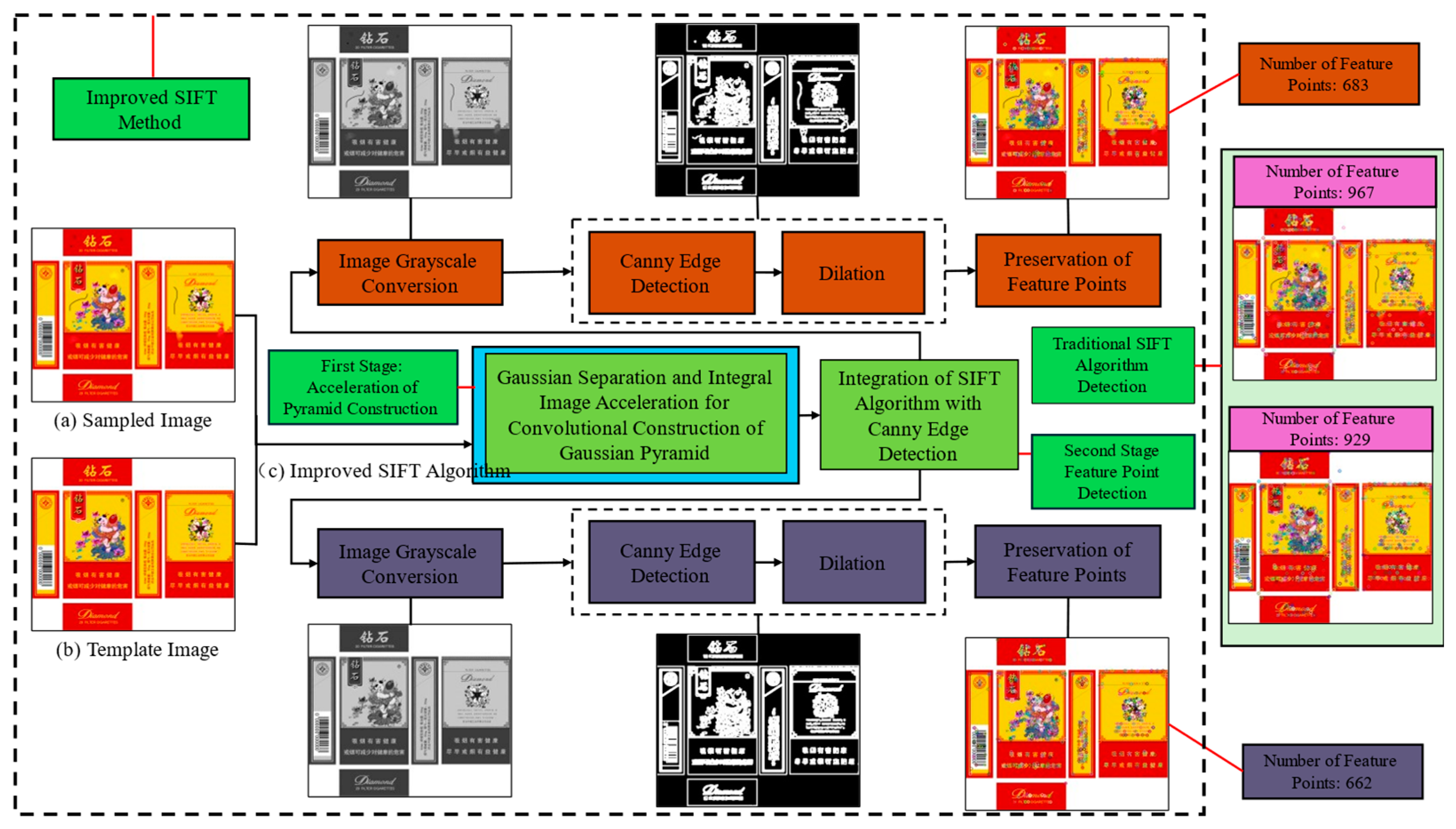
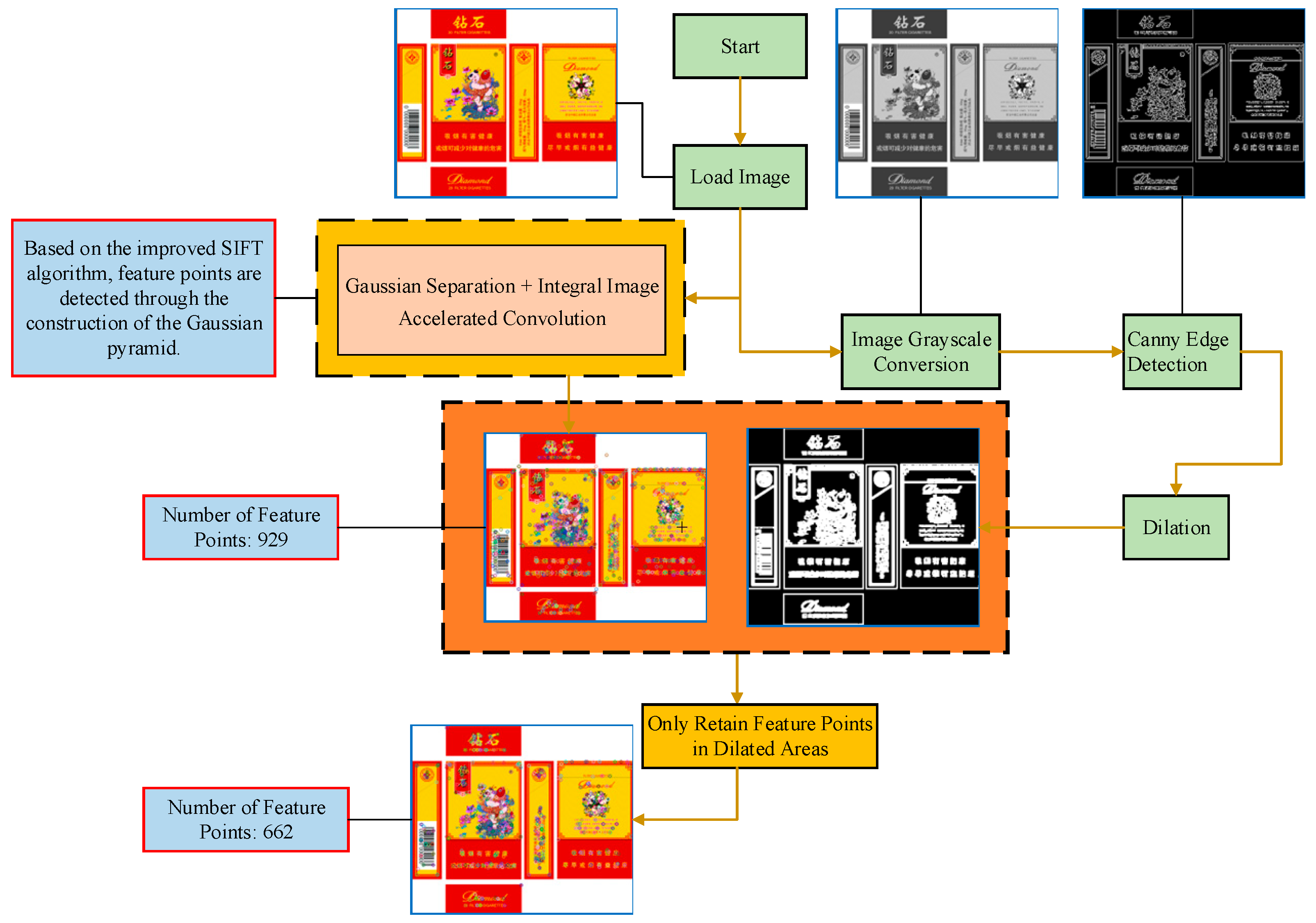
3.1. Improved Gaussian Pyramid Construction Based on SIFT
3.1.1. Gaussian Separation
3.1.2. Accelerated Convolution of Integral Images
3.2. Based on the Traditional SIFT Algorithm Integrated with Canny Edge Detection
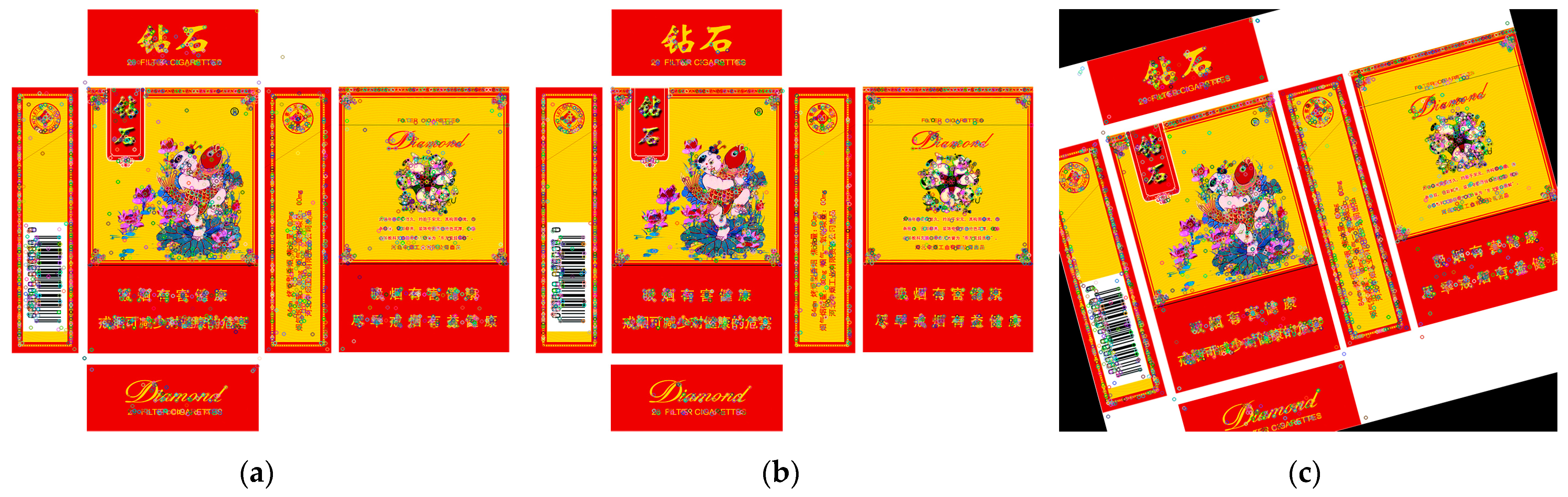
3.3. Image Alignment
- Initialization of Matched Pair Set: Start by forming a set from the feature point pairs of the two local images, labeled as N; then randomly select four matched pairs from N.
- Random Sample Selection: Since at least four points are needed to estimate an affine or perspective transformation, randomly choose four matched pairs from the set N.
- Model Parameter Solution: Based on these four pairs of points, calculate the eight unknown parameters in transformation Equation (20) to form a preliminary transformation matrix H.
- Error Calculation for Other Samples in Set N: Calculate the error for the other sample points in the set using the preliminary transformation matrix H. Set a threshold T; if the error is less than or equal to T, these points are identified as inliers, i.e., correct matches. Conversely, matches that do not meet this criterion are considered outliers.
- Inlier Set Formation: Group the matched pairs with an error less than T into the inlier set S and recalculate the transformation matrix H* using the least squares method from Equation (20).
- Iterative Optimization: Repeat the above process K times, retaining the transformation matrix with the highest number of inliers from each iteration. This matrix is considered the optimal spatial transformation model.
4. Experimental Evaluation
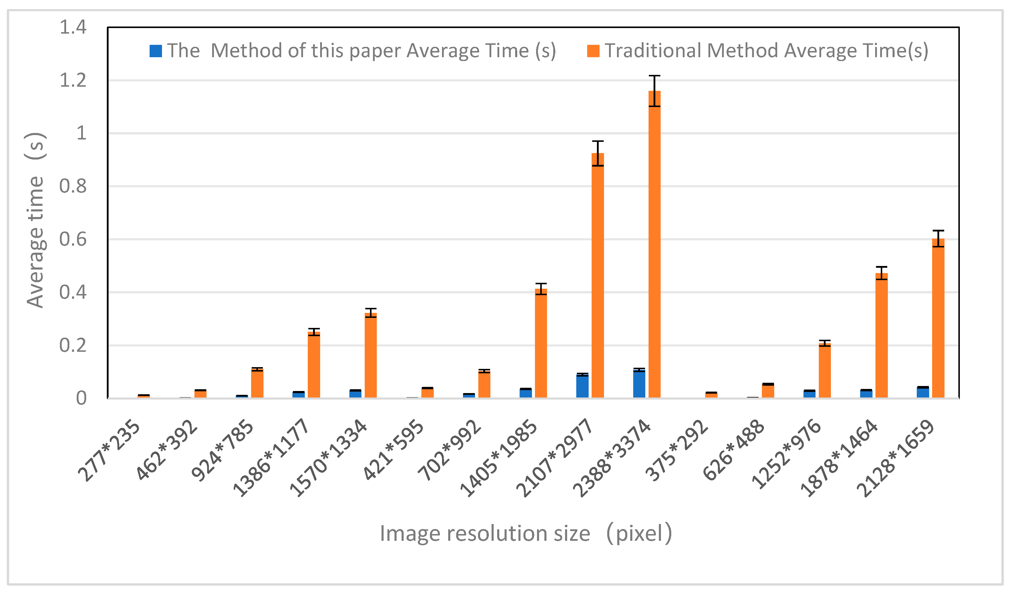
4.1. Experiment on the Efficiency of the Improved SIFT Gaussian Pyramid Construction
- Impact of Scaling Ratio: For both methods, as the scaling ratio increased from 0.3 times to 1.7 times, the processing time also increased, reflecting the increased complexity in building the Gaussian pyramid due to more pixels in enlarged images. However, the growth in construction time for the Gaussian pyramid in large images was more gradual with the improved SIFT method, demonstrating its efficiency in processing large images.
- Algorithm Adaptability and Stability: The improved SIFT method showed stable time growth across different image types and scaling ratios, indicating the adaptability and stability of the algorithm. In contrast, the traditional SIFT method had more significant time increases with specific image types and higher scaling ratios.
- Suitability for Application Scenarios: Due to its high efficiency and stability, the improved SIFT method is particularly well-suited for scenarios requiring fast and efficient processing, such as real-time image processing or in resource-limited environments.
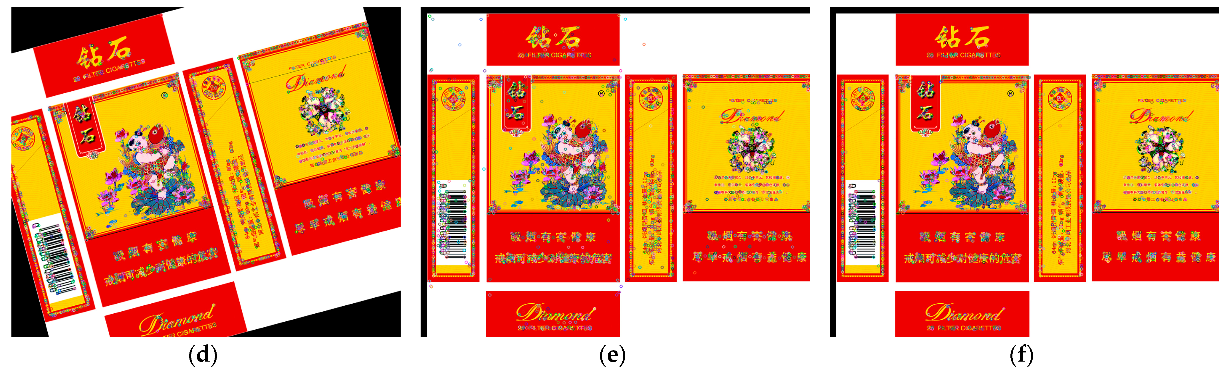
4.2. Experiment on Improved Keypoint Filtering Based on SIFT
4.3. Discussion
5. Conclusions
Author Contributions
Funding
Data Availability Statement
Acknowledgments
Conflicts of Interest
References
- Yang, H.; Li, X.R.; Zhao, L.Y.; Chen, S.H. A Novel Coarse-to-Fine Scheme for Remote Sensing Image Registration Based on Sift and Phase Correlation. Remote Sens. 2019, 11, 1833. [Google Scholar] [CrossRef]
- Li, J.W.; Wu, X.Y.; Liao, P.H.; Song, H.H.; Yang, X.M.; Zhang, Z.R. Robust Registration for Infrared and Visible Images Based on Salient Gradient Mutual Information and Local Search. Infrared Phys. Technol. 2023, 131, 104711. [Google Scholar] [CrossRef]
- Liang, H.D.; Liu, C.L.; Li, X.G.; Wang, L.N. A Binary Fast Image Registration Method Based on Fusion Information. Electronics 2023, 12, 4475. [Google Scholar] [CrossRef]
- Lu, J.Y.; Jia, H.G.; Li, G.; Li, Z.Q.; Ma, J.Y.; Zhu, R.F. An Instance Segmentation Based Framework for Large-Sized High-Resolution Remote Sensing Images Registration. Remote Sens. 2021, 13, 1657. [Google Scholar] [CrossRef]
- Liu, J.L.; Bu, F.L. Improved RANSAC Features Image-Matching Method Based on SURF. J. Eng.-JoE 2019, 23, 9118–9122. [Google Scholar] [CrossRef]
- Lazar, E.; Bennett, K.S.; Hurtado Carreon, A.; Veldhuis, S.C. An Automated Feature-Based Image Registration Strategy for Tool Condition Monitoring in CNC Machine Applications. Sensors 2024, 24, 7458. [Google Scholar] [CrossRef] [PubMed]
- Li, B. Application of Machine Vision Technology in Geometric Dimension Measurement of Small Parts.EURASIP. J. Image Video Proc. 2018, 127, 1–8. [Google Scholar] [CrossRef]
- Xin, Z.H.; Wang, H.Y.; Qi, P.Y.; Du, W.D.; Zhang, J.; Chen, F.H. Printed Surface Defect Detection Model Based on Positive Samples. Comput. Mater. Contin. 2022, 72, 5925–5938. [Google Scholar] [CrossRef]
- Ben-Zikri, Y.K.; Helguera, M.; Fetzer, D.; Shrier, D.A.; Aylward, S.R.; Chittajallu, D.; Niethammer, M.; Cahill, N.D.; Linte, C.A. A Feature-based Affine Registration Method for Capturing Background Lung Tissue Deformation for Ground Glass Nodule Tracking. Computer methods in biomechanics and biomedical engineering. Imaging Vis. 2022, 10, 521–539. [Google Scholar] [CrossRef]
- Kuppala, K.; Banda, S.; Barige, T.R. An Overview of Deep Learning Methods for Image Registration with Focus on Feature-Based Approaches. Int. J. Image Data Fusion 2020, 11, 113–135. [Google Scholar] [CrossRef]
- Razaei, M.; Rezaeian, M.; Derhami, V.; Khorshidi, H. Local Feature Descriptor using Discrete First and Second Fun-Damental Forms. J. Electron. Imaging 2021, 30, 023008. [Google Scholar] [CrossRef]
- Chang, H.-H.; Chan, W.-C. Automatic Registration of Remote Sensing Images Based on Revised Sift with Trilateral Computation and Homogeneity Enforcement. IEEE Trans. Geosci. Remote Sens. 2021, 59, 7635–7650. [Google Scholar] [CrossRef]
- Harris, C.G.; Stephens, M. A Combined Corner and Edge Detector. In Proceedings of the Alvey Vision Conference, Manchester, UK, 1 January 1988; pp. 147–151. [Google Scholar] [CrossRef]
- Lowe, D.G. Distinctive Image Features from Scale-Invariant Keypoints. Int. J. Comput. Vis. 2004, 60, 91–110. [Google Scholar] [CrossRef]
- Zheng, S.Y.; Zhang, Z.X.; Zhang, J.Q. Image Relaxation Matching Based on Feature Points for DSM Generation. Geo-Spat 2004, 7, 243–248. [Google Scholar] [CrossRef]
- Ke, Y.; Sukthankar, R. PCA-SIFT: A More Distinctive Representation for Local Image Descriptors. In Proceedings of the 2004 IEEE Computer Society Conference on Computer Vision and Pattern Recognition CVPR 2004, Washington, DC, USA, 27 June–2 July 2004. [Google Scholar] [CrossRef]
- Alhwarin, F.; Ristić-Durrant, D.; Gräser, A. VF-SIFT: Very Fast SIFT Feature Matching. In Pattern Recognition (DAGM 2010); Lecture Notes in Computer Science, Volume 6376; Goesele, M., Roth, S., Kuijper, A., Schiele, B., Schindler, K., Eds.; Springer: Berlin/Heidelberg, Germany, 2010. [Google Scholar] [CrossRef]
- Sedaghat, A.; Mokhtarzade, M.; Ebadi, H. Uniform Robust Scale-Invariant Feature Matching for Optical Remote Sensing Images. IEEE Trans. Geosci. Remote Sens. IEEE 2011, 49, 4516–4527. [Google Scholar] [CrossRef]
- Yu, Z.W.; Zhang, N.; Pan, Y.; Zhang, Y.; Wang, Y.X. Heterogeneous Image Matching Based on Improved SIFT Algorithm. Laser Optoelectron. Prog. 2022, 59, 1211002. [Google Scholar] [CrossRef]
- Zhu, F.; Zheng, S.; Wang, X.; He, Y.; Gui, L.; Gong, L. Real-Time Efficient Relocation Algorithm Based on Depth Map for Small-Range Textureless 3D Scanning. Sensors 2019, 19, 3855. [Google Scholar] [CrossRef] [PubMed]
- Yang, J.; Xiao, Y.; Cao, Z. Toward the Repeatability and Robustness of the Local Reference Frame for 3D Shape Matching: An Evaluation. IEEE Trans. Image Process 2018, 27, 3766–3781. [Google Scholar] [CrossRef]
- Bonnaffe, W.; Coulson, T. Fast fitting of neural ordinary differential equations by Bayesian neural gradient matching to infer ecological interactions from time-series data. Methods Ecol. Evol. 2023, 14, 1543–1563. [Google Scholar] [CrossRef]
- Yang, J.; Zhang, Q.; Xiao, Y.; Cao, Z. TOLDI: An effective and robust approach for 3D local shape description. Pattern Recognit. 2017, 65, 175–187. [Google Scholar] [CrossRef]
- Petrelli, A.; Di Stefano, L. Pairwise registration by local orientation cues. Comput. Graph. Forum 2016, 35, 59–72. [Google Scholar] [CrossRef]
- Liu, Y.Y.; He, M.; Wang, Y.Y.; Sun, Y.; Gao, X.B. Fast Stitching for The Farmland Aerial Panoramic Images Based on Optimized SIFT Algorithm. Trans. CSAE 2023, 39, 117–125. [Google Scholar] [CrossRef]
- Paul, S.; D., U.; Naidu, Y.; Reddy, Y. An Efficient SIFT-based Matching Algorithm for Optical Remote Sensing Images. Remote Sens. Lett. 2022, 13, 1069–1079. [Google Scholar] [CrossRef]
- Gao, S.P.; Xia, M.; Zhuang, S.J. Automatic Mosaic Method of Remote Sensing Images Based on Machine Vision. Comput. Opt. 2024, 48, 705–713. [Google Scholar] [CrossRef]
- Liu, Y.Y.; He, M.; Wang, Y.Y.; Sun, Y.; Gao, X.B. Farmland Aerial Images Fast-Stitching Method and Application Based on Improved SIFT Algorithm. IEEE Access 2022, 10, 95411–95424. [Google Scholar] [CrossRef]
- Tang, L.; Ma, S.H.; Ma, X.C.; You, H.R. Research on Image Matching of Improved Sift Algorithm Based on Stability Factor and Feature Descriptor Simplification. Appl. Sci. 2022, 12, 8448. [Google Scholar] [CrossRef]
- Sundani, D.; Widiyanto, S.; Karyanti, Y.; Wardani, D.T. Identification of Image Edge Using Quantum Canny Edge Detection Algorithm. J. ICT Res. Appl. 2019, 13, 133–144. [Google Scholar] [CrossRef]
- Niedfeldt, P.C.; Beard, R.W. Convergence and Complexity Analysis of Recursive-RANSAC: A New Multiple Target Tracking Algorithm. IEEE Trans. Autom. Control 2016, 61, 456–461. [Google Scholar] [CrossRef]


| The Traditional SIFT Gaussian Pyramid Construction Method with Images of Different Sizes | The Improved SIFT Gaussian Pyramid Construction Method | |
|---|---|---|
| feature point generation | generates a large number of feature points, robust but computationally expensive | reduces the number of feature points using Canny edge detection and dilation, maintaining robustness. |
| Gaussian pyramid construction | computationally intensive, involving multiple scales and octaves. | simplified using Gaussian separation techniques and accelerated with integral image technology |
| real-time performance | struggles to achieve real-time performance, especially for large-scale images | significantly improved real-time performance, suitable for large-scale images |
| time efficiency | high computational demand, long processing times. | reduced time for constructing the Gaussian pyramid and detecting feature points |
| accuracy | high accuracy in feature point detection and image registration. | maintains high accuracy while reducing computational load. |
| comparative experiments | consistently slower, especially for large images | consistently faster, regardless of image size or type |
| Image Type | Image Resolution Size (pixel) | Time for the Improved SIFT Gaussian Pyramid Construction Method | Time for the Traditional SIFT Gaussian Pyramid Construction Method | ||||||
|---|---|---|---|---|---|---|---|---|---|
| 1 | 2 | 3 | Average Time (s) | 1 | 2 | 3 | Average Time (s) | ||
| a | 277 × 235 | 0.0010 | 0.0010 | 0.0010 | 0.0010 | 0.0121 | 0.0127 | 0.0127 | 0.0125 |
| 462 × 392 | 0.0020 | 0.0020 | 0.0020 | 0.0020 | 0.0307 | 0.0301 | 0.0314 | 0.0307 | |
| 924 × 785 | 0.0090 | 0.0099 | 0.0110 | 0.0100 | 0.1108 | 0.1099 | 0.1099 | 0.1102 | |
| 1386 × 1177 | 0.0239 | 0.0239 | 0.0239 | 0.0239 | 0.2481 | 0.2559 | 0.2471 | 0.2504 | |
| 1570 × 1334 | 0.0299 | 0.0309 | 0.0299 | 0.0302 | 0.3196 | 0.3186 | 0.3287 | 0.3223 | |
| Average Time for Image Type a | 0.0134 | Average Time for Image Type a | 0.1452 | ||||||
| b | 421 × 595 | 0.0021 | 0.0023 | 0.0020 | 0.0021 | 0.0396 | 0.0379 | 0.0399 | 0.0391 |
| 702 × 992 | 0.0174 | 0.0160 | 0.0177 | 0.0170 | 0.1042 | 0.1029 | 0.1016 | 0.1029 | |
| 1405 × 1985 | 0.0383 | 0.0374 | 0.0313 | 0.0357 | 0.4054 | 0.4116 | 0.4214 | 0.4128 | |
| 2107 × 2977 | 0.0937 | 0.0937 | 0.0816 | 0.0897 | 0.9129 | 0.9247 | 0.9347 | 0.9241 | |
| 2388 × 3374 | 0.1094 | 0.1038 | 0.1094 | 0.1075 | 1.1615 | 1.1656 | 1.1499 | 1.1593 | |
| Average Time for Image Type b | 0.0504 | Average Time for Image Type b | 0.5276 | ||||||
| c | 375 × 292 | 0.0010 | 0.0011 | 0.0010 | 0.0010 | 0.0214 | 0.0213 | 0.0224 | 0.0217 |
| 626 × 488 | 0.0022 | 0.0022 | 0.0031 | 0.0025 | 0.0537 | 0.0534 | 0.0533 | 0.0535 | |
| 1252 × 976 | 0.0284 | 0.0288 | 0.0293 | 0.0288 | 0.2070 | 0.2075 | 0.2091 | 0.2079 | |
| 1878 × 1464 | 0.0312 | 0.0306 | 0.0327 | 0.0315 | 0.4668 | 0.4778 | 0.4733 | 0.4726 | |
| 2128 × 1659 | 0.0402 | 0.0433 | 0.0424 | 0.0420 | 0.6038 | 0.6032 | 0.6013 | 0.6028 | |
| Average Time for Image Type c | 0.0212 | Average Time for Image Type c | 0.2717 | ||||||
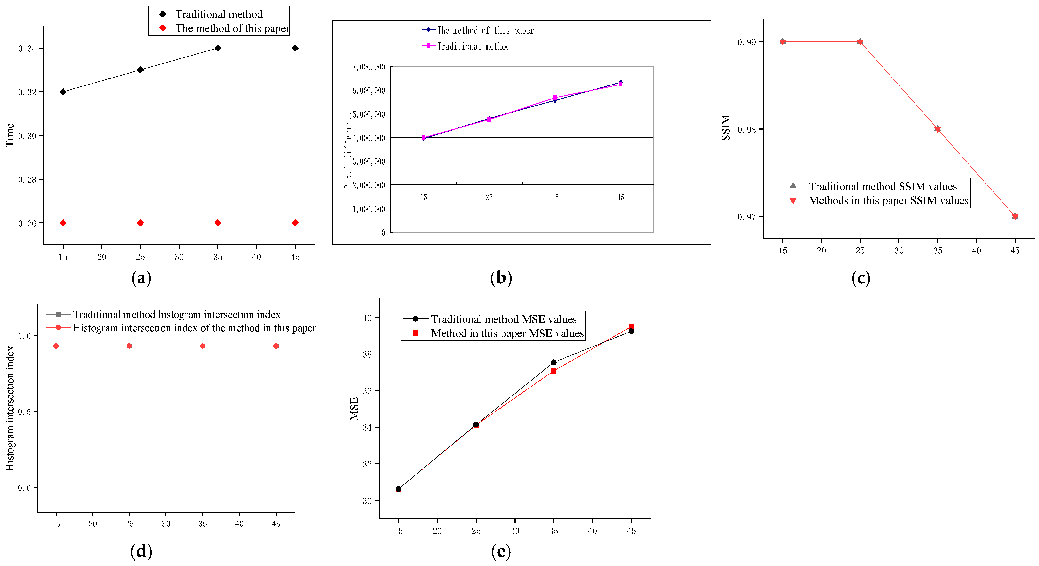
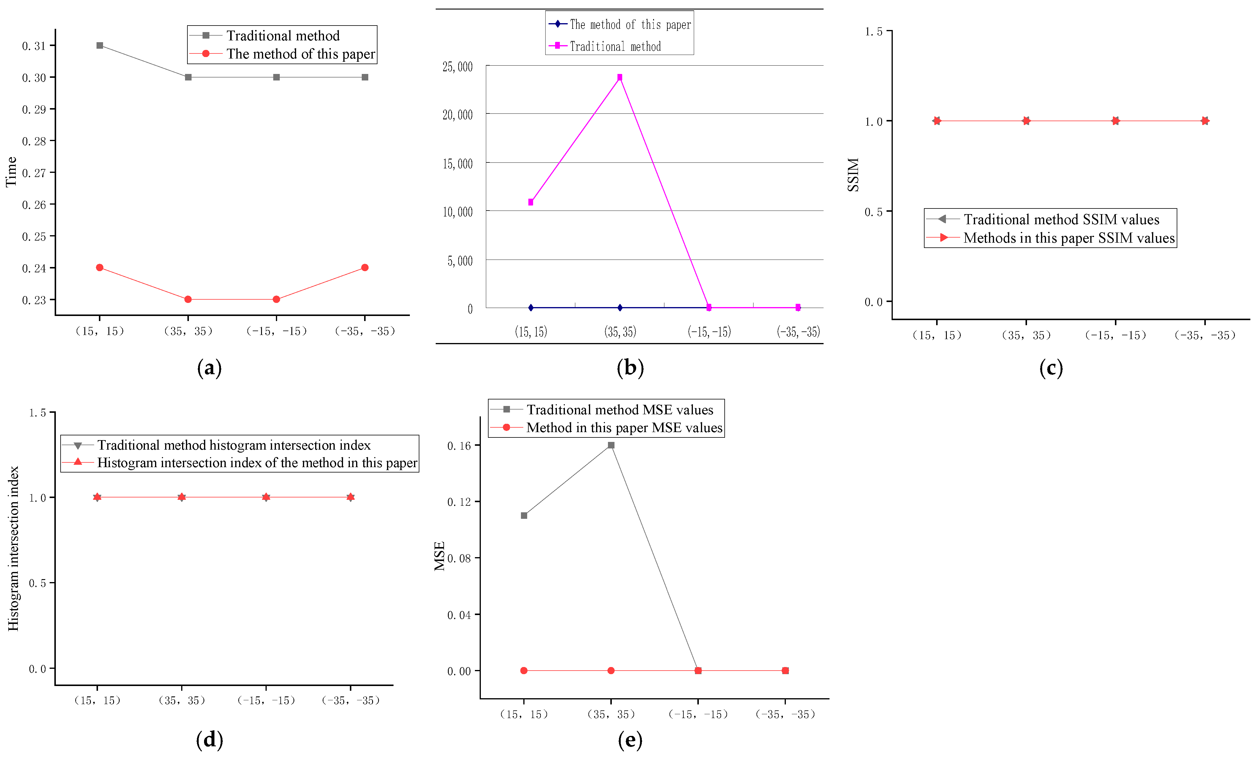
| Rotation Angle (°) | 15 | 25 | 35 | 45 | Translation Distance (mm) | (15, 15) | (35, 35) | (−15, −15) | (−35, −35) | |
|---|---|---|---|---|---|---|---|---|---|---|
| Number of keypoints after filtering | Image a | 2994 | 2900 | 2957 | 3071 | 2429 | 2358 | 2382 | 2317 | |
| Number of keypoints before filtering | Image a | 3685 | 3604 | 3638 | 3689 | 3124 | 3031 | 3087 | 2974 | |
| Time from feature point detection to image registration | The method of this paper | 0.26 | 0.26 | 0.26 | 0.26 | 0.24 | 0.23 | 0.23 | 0.24 | |
| Traditional method | 0.32 | 0.33 | 0.34 | 0.34 | 0.31 | 0.30 | 0.30 | 0.30 | ||
| Pixel difference | The method of this paper | 3,953,015 | 4,800,217 | 5,569,518 | 6,336,485 | 0 | 0 | 0 | 0 | |
| Traditional method | 4,000,647 | 4,762,046 | 5,671,722 | 6,241,591 | 10,853 | 23,716 | 0 | 0 | ||
| SSIM | The method of this paper | 0.99 | 0.99 | 0.98 | 0.97 | 1.0 | 1.0 | 1.00 | 1.00 | |
| Traditional method | 0.99 | 0.99 | 0.98 | 0.97 | 1.0 | 1.0 | 1.00 | 1.00 | ||
| MSE | The method of this paper | 30.62 | 34.11 | 37.07 | 39.50 | 0.0 | 0.0 | 0 | 0 | |
| Traditional method | 30.62 | 34.13 | 37.54 | 39.24 | 0.11 | 0.16 | 0 | 0 | ||
| Index | The method of this paper | 0.93 | 0.93 | 0.93 | 0.93 | 1.00 | 1.00 | 1.00 | 1.00 | |
| Traditional method | 0.93 | 0.93 | 0.93 | 0.93 | 1.00 | 1.00 | 1.00 | 1.00 |
Disclaimer/Publisher’s Note: The statements, opinions and data contained in all publications are solely those of the individual author(s) and contributor(s) and not of MDPI and/or the editor(s). MDPI and/or the editor(s) disclaim responsibility for any injury to people or property resulting from any ideas, methods, instructions or products referred to in the content. |
© 2025 by the authors. Licensee MDPI, Basel, Switzerland. This article is an open access article distributed under the terms and conditions of the Creative Commons Attribution (CC BY) license (https://creativecommons.org/licenses/by/4.0/).
Share and Cite
Li, Y.; Zhang, D. Toward Efficient Edge Detection: A Novel Optimization Method Based on Integral Image Technology and Canny Edge Detection. Processes 2025, 13, 293. https://doi.org/10.3390/pr13020293
Li Y, Zhang D. Toward Efficient Edge Detection: A Novel Optimization Method Based on Integral Image Technology and Canny Edge Detection. Processes. 2025; 13(2):293. https://doi.org/10.3390/pr13020293
Chicago/Turabian StyleLi, Yanqin, and Dehai Zhang. 2025. "Toward Efficient Edge Detection: A Novel Optimization Method Based on Integral Image Technology and Canny Edge Detection" Processes 13, no. 2: 293. https://doi.org/10.3390/pr13020293
APA StyleLi, Y., & Zhang, D. (2025). Toward Efficient Edge Detection: A Novel Optimization Method Based on Integral Image Technology and Canny Edge Detection. Processes, 13(2), 293. https://doi.org/10.3390/pr13020293