Abstract
This study evaluates the improvement of numerical accuracy in the PSA model for ethanol dehydration using molecular sieves. By incorporating cubic state equations for vapor density determination, significant errors were identified when applying the ideal gas assumption to the ethanol–water mixture, particularly under moderate pressure conditions. The integration of the Peng–Robinson equation demonstrated a 5–10% improvement in calculation accuracy compared to the ideal gas law. This enhancement is crucial for achieving reliable predictions under non-ideal conditions, enabling more accurate estimations of real process dynamics across varying scenarios. Notably, improved accuracy in the PSA model is essential for designing more efficient and reliable industrial applications, especially at moderate pressures. The results indicate that the Peng–Robinson equation provides a more accurate representation of the density of the ethanol–water vapor mixture, contributing significantly to more accurate simulation results of the PSA process.
1. Introduction
In recent years, global biofuel production, including ethanol, has experienced a significant increase, with the United States, Brazil, and China emerging as major producers. This growth stems from global energy reforms aimed at reducing greenhouse gas emissions in the medium and long term [1,2]. Ethanol, a highly sought-after raw material, distinguishes itself for its involvement in a diverse range of products, including solvents, refrigerants, preservatives, antiseptics, perfumes, alcoholic beverages, and fuels [3,4,5]. Fuel ethanol, a concentrated alcohol used as an additive to gasoline, undergoes purification processes to eliminate residual water from prior production stages. While distillation is the most common technology, followed by extractive distillation, dehydration by molecular sieves offers a more energy-efficient pathway [6]. However, areas for improvement and further development in this process still exist.
In molecular sieve adsorption processes, one or more components are extracted from a gas or liquid stream and adhered to the surface of a solid adsorbent. Industrial processes typically utilize solid particles arranged in a fixed packed bed. To separate a binary mixture into the adsorption column, the ethanol–water mixture undergoes pressurization and is fed through the bed. Figure 1 represents a schematic representation of the adsorption process where solid particles in the bed capture water from the blend in a step known as adsorption [7]. As the bed reaches saturation, the flow halts, requiring column regeneration. The bed can be either thermally regenerated or fed under vacuum pressure with recirculation of the enriched product and regenerated by the desorption process. This process, termed pressure swing adsorption (PSA), is extensively applied in separating gaseous mixtures [8]. In the liquid phase, it is focused on extracting organic compounds from water, while in the gas phase, it eliminates water from gaseous hydrocarbons and solvents from the air [9].
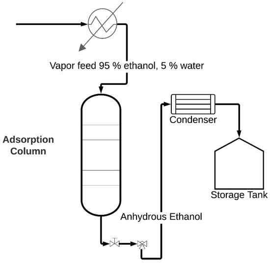
Figure 1.
Schematic representation of the ethanol dehydration process.
Understanding the thermodynamic properties of the pure components of the ethanol–water binary mixture is essential to improve the comprehension of ethanol dehydration. Density, a crucial parameter, has often been modeled using the ideal gas law in earlier investigations of pressure swing adsorption [10,11,12,13,14,15,16]. The literature offers information on the thermodynamic properties of the liquid phase [17] and includes experimental studies on the viscosity of ethanol at temperatures ranging from 298.15 to 328.15 K [18]. Additionally, there are studies related to binary benzene–ethanol or water–ethanol mixtures [19,20], applications of state equations associated with the study of the ethanol liquid phase [21,22], and works correlated to the study of the specific volume of ethanol mixtures and other alcohols in liquid phase in temperature ranges from 273.15 to 480 K at different pressures [23]. Studies carried out for alcohols in pure state are reported [24,25,26,27,28] at pressures of 2763.39 atm [29,30] and temperatures from 310 to 480 K at 1973.85 atm [31,32,33]. There are also studies of thermodynamic properties near to the critical point [34,35,36]. However, information regarding ethanol in the gas phase is limited compared to studies in the liquid phase [37].
The Peng–Robinson equation [38] emerges as a viable and extensively used option in the oil industry for predicting the thermodynamic properties of both pure components and binary mixtures [39]. In this research, the error linked to applying the ideal gas law equation for calculating the density of an ethanol–water vapor mixture in the numerical solution of the PSA model was contrasted again with those derived using the Peng–Robinson equation, uncovering more precise outcomes resulting from the inclusion of a more rigorous state equation, including a correlation for binary interaction parameters in gaseous mixtures. Proposing the integration of these elements into the numerical solution of pressure swing adsorption introduces a novel concept, given that the existing model heavily relies on the perfect gas law equation, effective under atmospheric conditions at high temperature. However, our investigation demonstrates that, even at moderate pressure (<10 atm), this error becomes significant. Studies simulating adsorption by molecular sieves for the separation of ethanol–water mixture typically assume the ideal gas equation. Our work challenges this assumption, highlighting its limitations, particularly under moderate-elevated pressures.
Earlier investigations into adsorption models have thermal effects associated with water adsorption in a packed column with zeolite 3A using a temperature swing adsorption model [4]. For pressure swing adsorption models, Kupiec et al. [7] performed a theoretical analysis, verifying it experimentally at a laboratory scale, demonstrating concordance between experimental and simulation results at a temperature of 373.15 K and 1 atm. In their investigation of water removal from ethanol, Gutiérrez-González et al. [40] solved two mathematical models and evaluated breakthrough curves at pressures of 3 atm and 433 K. Karimi et al. [13] formulated the numerical solution for a PSA model to separate an ethanol–water binary mixture, analyzing breakthrough curves for the molar fraction of water under various operational conditions. Rumbo Morales et al. [14] introduced a control structure for an adsorption process using a non-linear mathematical model and designed two controllers (Optimal MPC and Fuzzy PD + I) with the primary objective of maintaining optimal ethanol purity for use as a fuel.
This study demonstrates that existing equations of state reported in the literature fail to accurately represent the binary behavior of water and ethanol at moderated and high temperatures. Consequently, we assessed the use of rigorous methods that integrate the Peng–Robinson equation with correlations for binary interaction parameters in gaseous mixtures. By incorporating this approach, the accuracy of density calculations in the pressure swing adsorption (PSA) model for ethanol dehydration is significantly enhanced. When compared with experimental data using zeolite 3A as the adsorbent, the Peng–Robinson equation reduced prediction errors by 5–10% compared to the ideal gas law. These findings provide critical insights into designing PSA processes in industrial applications, where accurate thermodynamic predictions are essential for assessing operational efficiency. The main contribution of this paper is addressing the problem of determining, through exhaustive numerical evaluations, whether the additional computational cost of incorporating a rigorous cubic state equation is justified for solving a PSA process model using a finite difference algorithm. Furthermore, these findings aim to be valid for any type of computational finite element algorithm. This paper is structured as follows: Section 2 outlines the preliminary problem formulation, mathematical model and process parameters, and solution methodology. In Section 3, we present results and engage in discussions of numerical findings, which were validated using experimental data from the literature covering a temperature range of 373.15 K to 1573.15 K and pressures from 0.1 atm to 4 atm. Finally, Section 4 provides the conclusions.
2. Preliminaries and Problem Formulation
2.1. Preliminary Problem Formulation
The motivation for this study stems from the crucial need to incorporate a rigorous state equation to compute gas-phase density in water–ethanol mixtures. This is essential for improving the accuracy in the numerical analysis of ethanol dehydration process through adsorption [4,7,11,14]. The existing literature predominantly employs the ideal gas equation (Equation (1)) for density calculations [4,7,10,11,40]. The extensive use of the ideal gas equation in prior studies underscores the need to make a transition towards a more rigorous state equation which aims to enhance the precision of gas-phase density calculations in the numerical solution of the ethanol dehydration process via adsorption.
The proposed addition of a more rigorous state equation was implemented and validated using existing data from the literature for the binary mixture. The experimental data available in the literature reveals extensive studies conducted in the liquid phase [36]. Despite the wealth of information in the liquid phase, limited data exists on the density of the gaseous phase water–ethanol mixtures [36,40], and there is similarly scarce literature for pure components. The lack of sufficient experimental information makes it impractical to calculate this parameter using a specialized simulator. Instead, our approach focuses on the integration of a FORTRAN language programming code capable of calculating density as functions of pressure, temperature, and binary mixture composition. This strategy aligns with the goal of developing a practical solution for the numerical solution of the pressure swing adsorption mathematical model.
The following comments are in order to justify the use FORTRAN language in this research. Despite the existence of more modern programming languages, such as Python and C++, FORTRAN was chosen for this study due to its proven efficiency in solving complex numerical problems in scientific simulations. FORTRAN has stood the test of time and continues to be widely used in both industry and academia for high-precision calculations. Its optimized performance in numerical computations, particularly in handling large datasets and solving advanced mathematical models, makes it an ideal choice for simulations like pressure swing adsorption (PSA). Moreover, FORTRAN is highly compatible with optimized mathematical libraries, which facilitated the implementation of the PSA model and the integration of rigorous state equations in this research. The decision to use FORTRAN also reflects its historical and continued relevance in scientific computing, particularly in fields that require robust numerical solutions.
2.2. Mathematical Model
A mathematical model, based on rigorous mass and momentum balances, is considered for the purpose of efficiently separating water from a binary mixture containing 95% ethanol and 5% water. The adsorption process employs clinoptilolite zeolite as the adsorbent agent and operates under precisely controlled isothermal conditions, with the objective of producing anhydrous ethanol, as detailed by Kupiec et al. [4]. The assumption of a constant process temperature, both in time and space, serves as a foundational element in this comprehensive mathematical model. The key assumptions guiding this model include:
- Only one component is adsorbed from the ethanol–water mixture.
- The pressure drop in the column packing adheres to the Ergun equation.
- Adsorption equilibrium conforms to the Dubinin–Radushkevich equation.
- Mass transfer resistance in the gas phase is considered negligible.
- Dispersion effects in the gas stream are deemed negligible.
- Adsorbent granules are assumed to have a spherical shape.
- The process is maintained as isothermal throughout.
- The mass transfer within the granule is appropriately described by the homogeneous diffusion mass transfer model.
- The kinetics of mass transfer within the granules are effectively described by the linear driving force (LDF) model.
- The temperatures of both phases remain constant over both time and space.
The equations governing this model (Equations (2)–(8)) [4,7] stem from a set of fundamental balances. The general mass balance is expressed as follows:
The water mass balance is articulated by the following:
The momentum balance equation can be described as the following:
The general mass balance takes into account various factors such as superficial velocity (u), pressure (P), bed porosity (ε), pellet density (p), gas density (g), ideal gas constant (R), temperature (T0), average equilibrium water content (), averaged bed water content (), molar mass of water (Mw), molar mass (M), and mass transfer coefficient in solid phase (ksa). The model comprehensively reflects the intricate relationship between these variables, offering insights into the adsorption process. Similarly, the water mass balance introduces additional elements such as the change in the water mol fraction (). This equation captures the dynamic behavior of water vapor within the adsorption system, considering factors like bed porosity, pellet density, gas constant, temperature, molar mass mixture, mass transfer coefficient, average equilibrium water content (), and current content water (). The momentum balance equation further extends the model by encompassing the Ergun equation, which operates under both laminar and turbulent flow conditions. This inclusion introduces parameters like gas viscosity (), the diameter of adsorbent pellet (), and gas density (). The Ergun equation plays a pivotal role in describing pressure drop within the packed column, offering a comprehensive representation of momentum dynamics. Additionally, other pivotal equations for this mathematical model include the Dubinin–Raduschkevich (D-R) (Equation (5)) equation, which characterizes adsorption equilibrium, relating the pellet equilibrium water content () to process temperature, pressure, and concentration.
The linear driving force equation (LDF) (Equation (6)) is another crucial element, employed to elucidate the mas transfer rate. This amalgamation of equations forms the backbone of the mathematical framework, facilitating a comprehensive understanding of the adsorption process and its dynamics.
The initial conditions at the beginning of adsorption step are as follows (Equation (7)):
The boundary conditions for the adsorption step are determined by the feed conditions to the adsorption system (Equation (8)):
The complete dataset used for solving the mathematical model (2)–(8), along with its respective sources, is available in reference [40]. This dataset has not been included in this paper to avoid unnecessary length and to maintain focus on the key results.
2.3. Cubic State Equation Parameters
Density calculation for a pure component using the Peng–Robinson equation requires knowledge of critical properties, including pressure and temperature, as well as the acentric factor specific to the component under evaluation. Furthermore, in the case of a binary mixture, the program incorporates a correlation to calculate binary interaction parameters (kij). Equation (9) embodies the Peng–Robinson equation, a cornerstone in the field of thermodynamics and widely used in chemical engineering studies [37,38,39,40,41]. This equation provides a robust framework for predicting thermodynamic properties, offering a comprehensive and accurate approach for density calculations essential for the numerical solution of the ethanol dehydration process via adsorption.
In Table 1, the critical properties of water and ethanol are summarized [42]. These properties are essential for the calculations in the Peng–Robinson equation, which will be used to predict the thermodynamic behavior of these components under various conditions. Understanding these properties is crucial for accurately modeling the density and other related thermodynamic properties in the pressure swing adsorption (PSA) process for ethanol dehydration.

Table 1.
Critical properties of water and ethanol.
To calculate density, the program uses Equations (10)–(12) for the calculation of P-R equation parameters of pure components [39]. For the calculation of density in a binary mixture, it is imperative to consider the correlation outlined in Equations (12)–(15) [39].
Equations (12) and (13) introduce binary empirical parameters aimed at enhancing the accuracy of predicting mixture thermodynamic properties while preserving the predictive nature of the procedure. The correlation guiding this process is expressed as follows:
Here denote the critical compressibility factors for both components. For the binary mixture, parameters and are replaced by and with the following mixing rules [26].
To calculate density in the adsorption column, the Fortran language program requires operating pressure and temperature. In cases involving the calculation of water–ethanol mixture density, the program employs specific instructions using the fixed-point method to compute the specific volume and subsequently obtain mixture density. The fixed-point method is an iterative scheme based on the rearrangement of a function f(x) = 0, where the variable x is rearranged explicitly:
Equation (18) provides a formula to predict a new value of x (specific volume) based on its value in the previous iteration [43]. With a given initial value for the root xi, Equation (18) is used iteratively to obtain a new approximation xi+1, as shown in the following iterative formula (Equation (19)) [43]:
The method requires the calculation of the approximate error using the normalized error formula (Equation (20)) [43]:
2.4. Solution Methodology
The solution methodology for developing the software for the numerical solution of pressure swing adsorption (PSA) model in the ethanol dehydration process is outlined in the following stages:
- Stage 1: Implementation of the Peng–Robinson equation.
In the initial stage, the sourced code for the Peng–Robinson equation (Equation (9)) has been implemented as a function module in a subroutine (Equation (21)).
This equation plays a crucial role in accurately calculating the density of the gaseous state ethanol–water binary mixture with predetermined precision. It is a function of temperature, pressure, and composition of the binary mixture.
- Stage 2: Subroutines for specific volume and density calculation.
The second stage involves creating two subroutines that utilize the fixed-point iterative method to calculate the specific volume and density in the numerical solution calculations (Equations (9)–(17)).
- Stage 3: Integration of subroutines and function.
In the third stage, we integrated the subroutines and the Peng–Robinson function. This requires grouping variables into program modules and declaring them as common blocks since they intervene in the FUNCTION module of the Peng–Robinson equation, initial conditions values for the finite difference method, and subroutines for the fixed-point method. The complete programming code of the mathematical model of pressure swing adsorption (Equations (2)–(8)) employs the centered finite difference method to discretize Equations (2)–(6). The finite difference method consists of transforming each partial differential equation into a set of ordinary differential equations, which are then solved by the fourth-order Runge–Kutta method. The program provides results such as breakthrough curves (molar fraction of water at the outlet of the adsorption column), initial density at the entrance of the adsorption column, and the density of the binary mixture during the numerical solution calculations. Figure 2 illustrates the steps and instructions executed by the program to solve the numerical method and obtain the density.
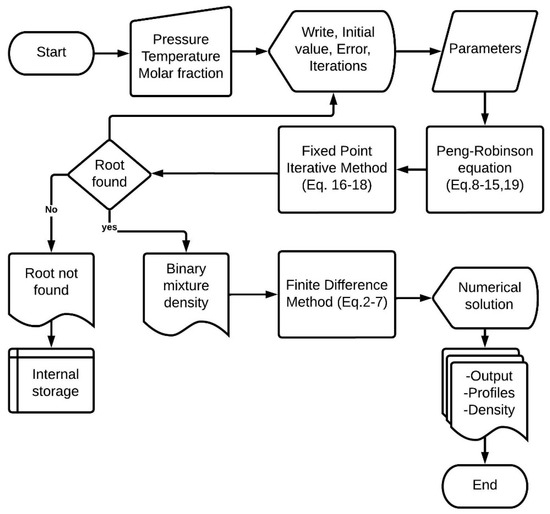
Figure 2.
Flowchart of the program in FORTRAN language.
To validate the program results, we conducted a literature review to obtain databases of water–ethanol density in the gaseous state. While the available literature had limited information, we compared the program’s calculated data with experimental data.
3. Results
In this section, the results of the programming code for calculating vapor mixture density within the available experimental data range are evaluated, with a comparison between the calculated results and experimental data for pure water and ethanol vapor. The program records numerical data in .dat format, enabling detailed graphical analysis. The testing and implementation phase involved various checks to ensure the accuracy and reliability of the program, as outlined below.
Density calculation for pure components:
- Calculation of water density and comparison with experimental data of superheated water vapor reported by Cengel and Boles [44] at different specified pressures and temperatures.
- Calculation of water density and comparison with experimental data of vapor water reported by [35] and the International Association for the Properties of Water and Steam (IAPWS) [45] at different specified pressures and temperatures.
- Calculation of ethanol density and comparison with experimental data of vapor ethanol reported by the International Association for the Properties of Water and Steam (IAPWS) [45] at different specified pressures and temperatures.
- Extrapolation of vapor water density to the experimental conditions reported in the International Association for the Properties of Water and Steam (IAPWS) [45] for vapor ethanol.
- Extrapolation of ethanol density in gaseous phase to the experimental conditions reported in Cengel and Boles [44] for vapor water.
- Graphical comparison of extrapolated data with experimental data reported in the literature.
- Comparison of calculated density for superheated water vapor by the Peng–Robinson equation, ideal gas equation, and experimental data consulted in the literature.
- Calculation of percentage error of results by the ideal gas equation with respect to experimental data.
- Evaluation of breakthrough curves obtained with the implemented subroutines.
- Results from the molar fraction of water at the outlet of the adsorption column at different specified pressures, compositions, and temperatures.
- Calculation of the feed density of the water–ethanol mixture.
- Density calculation throughout the simulation process.
Density Comparison for Pure Components
The results presented in Table 2 correspond to the calculations performed with the program for superheated vapor water across for pressures ranging from 0.098 to 0.98 atm at different temperatures. The table compares the numerical values obtained for the density in kg/m3 with those reported in the literature by Cengel and Boles [44].
Table 2.
Comparisons of calculated density with literature data for superheated steam.
Table 3 corresponds to the calculations performed with the program for superheated vapor water across for pressures ranging from 1.97 to 3.94 atm at different temperatures. The table compares the numerical values obtained for the density in kg/m3 with those reported in the literature by Cengel and Boles [44].
Table 3.
Comparisons of the calculated density with the literature for superheated steam.
The evaluation of superheated steam density, as outlined in Table 2 and Table 3, demonstrates a close alignment between the calculated density and the literature data reported by Cengel and Boles [44], indicating the effectiveness of this methodology in capturing the thermodynamic behavior of superheated stream. In Table 4, a detailed comparison is presented, juxtaposing our results with those obtained by Bazaev et al. [35] and the International Association for the Properties of Water and Steam (IAPWS) [45].
Table 4.
Test measurements of pure water density.
Table 5 and Table 6 present the calculated density for vapor ethanol, comparing it with literature data from the International Association for the Properties of Water and Steam across various pressure and temperature values [45].
Table 5.
Calculated density for pure state ethanol compared to the literature for a pressure range of 1.6–2.2 atm and a temperature range of 373 to 388 K.
Table 6.
Calculated density for pure state ethanol in pure state compared to the literature for a pressure range of 0.5–3.1 atm and a temperature range of 398 to 400 K.
Table 5, Table 6 and Table 7 collectively reveal a close alignment between the calculated numerical results for vapor phase ethanol and the experimental data reported in the literature (Wilson et al. [41]). An integral aspect to contemplate in this research is the feasibility of extrapolation beyond the existing experimental dataset. This observation highlights the robust performance of the employed methodology in accurately determining the density of the ethanol density across various temperature and pressure ranges. This confirmation further solidifies its applicability beyond the initially measured conditions.
Table 7.
Calculated density for pure state ethanol in pure state compared to the literature for a pressure range of 0.7–2.9 atm and a temperature range of 423 to 473 K.
In Figure 3, approximate results are observed compared to those presented in the literature for specific temperature and pressure conditions. The figure represents extrapolated density for vapor water under the pressure and temperature conditions reported by Wilson et al. [41] for superheated water vapor and experimental data evaluated by Smith et al. [42]. A noticeable agreement becomes apparent when the numerical results obtained with the Fortran program are graphically compared to the literature datasets, highlighting the validity and precision of the methodology employed and substantiating the program’s capability to effectively capture the thermodynamic behavior of water vapor density under superheating conditions.
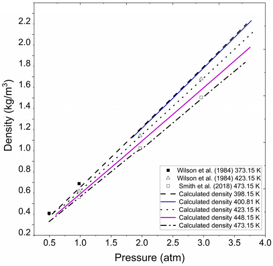
Figure 3.
Calculated water vapor density at different pressure and temperatures. Wilson et al. (1984) [41], Smith et al. (2018) [42].
Figure 4 presents the extrapolated density data obtained for vapor ethanol under the pressure and temperature conditions reported by Cengel and Boles [44] for superheated water and experimental data consulted in Wilson et al. [41]. The figure underscores the adaptability of the methodology to handle extrapolated density calculations for ethanol in the vapor phase, confirming its capability to deliver accurate results across varying thermodynamic conditions.
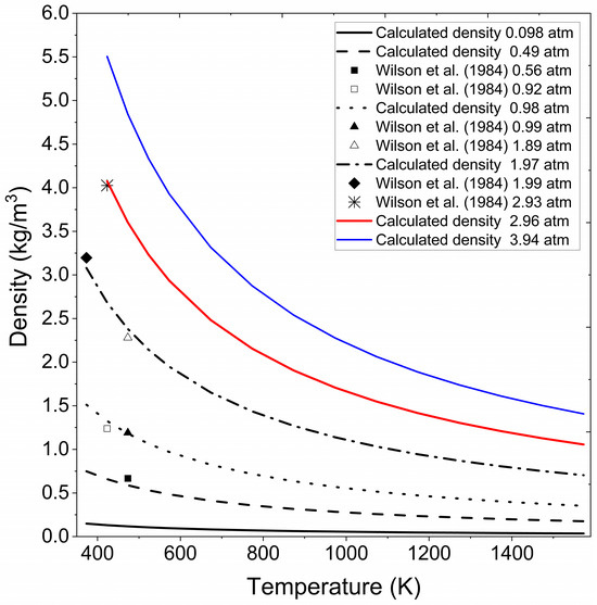
Figure 4.
Calculated ethanol vapor density at different pressures and temperatures. Wilson et al. (1984) [41].
In Figure 5, the results calculated by the Fortran program, utilizing the perfect gas law equation and the Peng–Robinson equation, are illustrated in comparison with experimental data reported by Cengel and Boles [44] from Table 2 and Table 3 for superheated water. It is noteworthy that a deviation increases between the experimental calculated data as pressure increases and temperature decreases, particularly with the ideal gas equation.
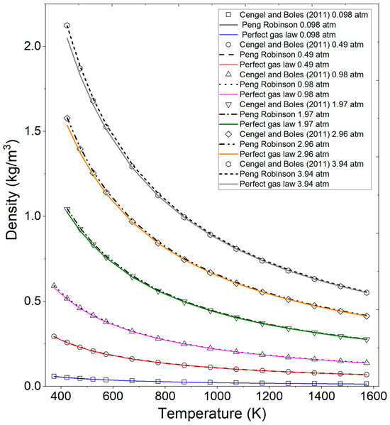
Figure 5.
Comparison of calculated ethanol vapor density by the ideal gas equation, Peng–Robinson, and the literature data at various pressures and temperatures. Cengel and Boles (2011) [44].
Figure 6 represents the data obtained by the FORTRAN program and data reported by Wilson et al. [41] from Table 5 for vapor ethanol with the Peng–Robinson equation. The results are also compared with the ideal gas equation under the same conditions employed by Wilson et al. [41]. It is evident that as pressure increases, the calculations by the ideal gas equation become less accurate. Therefore, if higher pressures studies are intended, the ideal gas equation is not a suitable alternative for continued use in mathematical models, particularly in pressure swing adsorption for ethanol dehydration processes. On the other hand, the Peng–Robinson equation more accurately calculates the density for ethanol and water under the experimental conditions used in the literature.
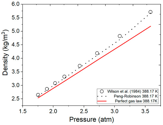
Figure 6.
Comparison of calculated ethanol vapor density by the ideal gas equation, Peng–Robinson, and the literature data at various pressures at a temperature of 388.17 K. Wilson et al. (1984) [41].
Figure 7 shows the percentage error from the calculated data using the ideal gas law concerning the experimental data in Table 5, Table 6 and Table 7 as well as Figure 6. The figure reveals that the error increases with rising operating pressure. While the error may not be a significant factor when handling vacuum or atmospheric pressure, it becomes noteworthy when exceeding 1.5 atmospheres. Specifically, at pressures greater than 2 atmospheres, the calculated error exceeds 3%, and at a temperature of 373.07 K and pressures surpassing 1.5 atm the error surpasses 4.5%. Between temperature range of 373.07 and 400.81 K, and pressures ranging from 0.5 to 3.5 atmospheres, the calculated error reaches 9% as the operating pressure increases. This observation is crucial, especially considering the operating pressures involved in pressure swing adsorption processes for ethanol dehydration reported in previous studies [7,13,14,37]. At low pressures, the density calculated by the ideal gas law may not significantly affect the PSA model. However, at moderate pressure, it becomes a crucial factor to consider. Therefore, the inclusion of a more rigorous state equation, such as the Peng–Robinson equation, in the calculation of the water–ethanol vapor mixture density would complement studies of ethanol dehydration process. Until this point, the presented results encompass stages 1 and 2 of Section 2.4: Solution Methodology.
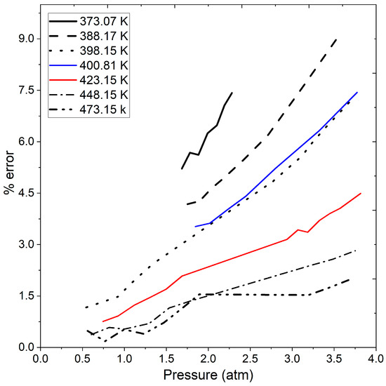
Figure 7.
Calculated error in ethanol vapor density by ideal gas law compared to experimental data at different pressures and temperatures.
The following results showcase the integration of the function and subroutine modules for the Peng–Robinson equation and the fixed-point iterative method into the PSA model code; this corresponds to the stage 3 of solution methodology. The numerical results obtained through the developed PSA simulator are depicted in Figure 8.
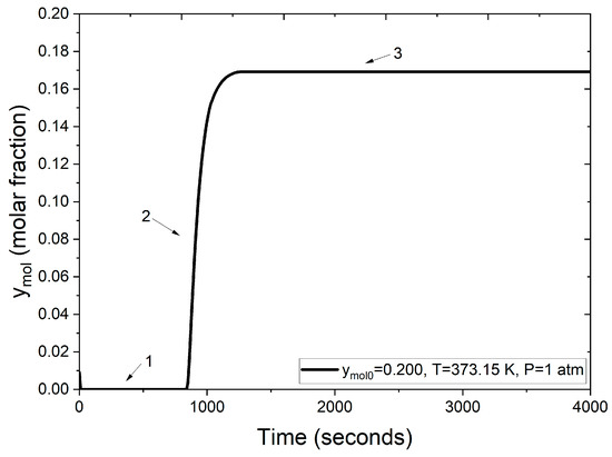
Figure 8.
Molar fraction of water at the adsorption column outlet.
Figure 8 illustrates the breakthrough curve stages (numbers 1–3) for the water–ethanol mixture during the PSA process, highlighting the adsorption efficiency of zeolite clinoptilolite.
- Section 1: Initially, the molar fraction of water at the outlet is zero. This indicates complete retention of water molecules within the packed bed, achieved by adsorption into the zeolite clinoptilolite. This behavior persists for approximately the first 900 s, signifying the high affinity and selective adsorption of water due to the zeolite’s pore size, which is compatible with the molecular dimension of water.
- Section 2: Beyond 900 s, the molar fraction of water at the outlet begins to rise. This increase is due to the progressive saturation of the zeolite clinoptilolite’s adsorption sites. As these cavities fill, the capacity to retain additional water diminishes, allowing more water molecules to pass through the adsorption column.
- Section 3: After roughly 1000 s, the adsorption sites within the zeolite clinoptilolite are fully saturated with the water molecules. This saturation reflects that the adsorbent can no longer retain additional water. Consequently, the water concentration at the outlet aligns with the feed concentration.
Figure 8 demonstrates the dynamic behavior of the adsorbent bed during the PSA process, confirming the effectiveness of zeolite clinoptilolite for molecular water retention and validating the employed model. The breakthrough curves, as evaluated in Figure 9, compare the numerical solutions obtained using two different approaches: one employing the ideal gas law and the other utilizing the Peng–Robinson equation, both under identical operating conditions (1 atm, 373 K and a feed mole fraction of 0.200 of water concentration). Figure 9 illustrates that under the same conditions, the process reaches bed saturation in approximately 500 s when density is calculated using the ideal gas law. In contrast, when employing the Peng–Robinson equation, the process takes almost twice as long, as shown in Figure 8.
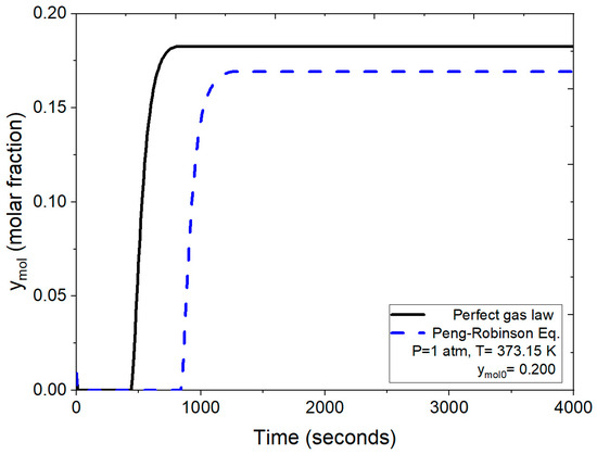
Figure 9.
Comparison of the mole fraction of water at the outlet using the ideal gas equation and the Peng–Robinson equation at 1 atm.
In this scenario, water presented in the binary mixture is effectively retained, ridding the mixture of water for about 900 s. Subsequently, as the molar fraction of water starts to increase, the feed water concentration is eventually reached at the process output; that is, there is no water retention after saturation is reached. This observed behavior closely aligns with experimental breakthrough curves reported by Leo-Avelino et al. [46] where similar conditions regarding particle size and the adsorbent agent (zeolite clinoptilolite) were employed. Both studies show a consistent adsorption process, with the packed bed reaching saturation at 900 s. It is noteworthy that the numerical solution presented here is based on implementing the Peng–Robinson equation. Comparatively, breakthrough curves reported by Kupiec et al. [7], Rossi et al. [14], and Gutierrez-Gonzalez et al. [40] were derived using a mathematical model with the ideal gas law for binary mixture density at atmospheric pressure conditions. The results obtained for natural zeolite clinoptilolite exhibit similarities to those presented for artificial zeolites in the works of Kupiec et al. [7] and Kupiec et al. [4].
The breakthrough curves depicted in Figure 10 compare the results obtained under identical operating conditions (2 atm, 370.02 K and ymol0 = 0.200 for water concentration) using both the numerical solution incorporating the ideal gas law and the one employing the Peng–Robinson equation for the density calculation. Under these conditions, as per the ideal gas law, the process leading to bed saturation initiates saturation around 200 s, culminating complete saturation at 435 s. In contrast, applying the more rigorous Peng–Robinson equation initiates saturation at approximately 490 s.
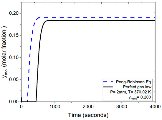
Figure 10.
Comparison of the mole fraction of water at the outlet using the ideal gas equation and the Peng–Robinson equation at 2 atm.
Figure 11 presents a comparison between the experimental data reported by Leo-Avelino et al. [46] and the numerical solution for the adsorption process using Mexican zeolite clinoptilolite. The experimental data includes results for three different types of zeolites: Zeolite #1, Zeolite #2, and Zeolite #3. The numerical solution accounts for various conditions, including particle size, feed water concentration, bed porosity, column dimensions, and the adsorbent agent. The comparison reveals a similar pattern during the adsorption stage, with the packed bed reaching saturation in approximately 1480 s for the numerical solution. This closely aligns with the experimental data for Zeolite #1 and Zeolite #3. Notably, the experimental data for Zeolite #2 shows a slightly higher molar fraction of water at earlier times, indicating a faster breakthrough compared to the other zeolites and the numerical solution. The use of the Peng–Robinson equation in the numerical model is crucial as it provides a more accurate representation of the thermodynamic properties of the ethanol–water mixture under varying conditions. This accuracy is reflected in the close agreement between the numerical and experimental results, the slight discrepancies observed with Zeolite #2 might be attributed to variations in particle size, feed concentration, or other experimental conditions not fully captured in the model.
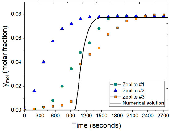
Figure 11.
Comparison of molar fraction of water at the outlet using the ideal gas equation and the Peng–Robinson equation at 2 atm.
In comparison, Gutiérrez-González et al. [40] observed similar breakthrough behavior using PSA model for ethanol dehydration, which did not initially incorporate the Peng–Robinson equation. The inclusion of this equation in the present study’s model has clearly enhanced the accurateness of the numerical solution, bringing it closer to the experimental data. The alignment of the numerical results with the experimental data underlines the effectiveness of the Peng–Robinson equation in improving the simulation accuracy for predicting the adsorption behavior of water–ethanol mixture using Mexican clinoptilolite. This enhancement is critical for capturing the dynamic behavior of the adsorption process, confirming its applicability in practical scenarios for ethanol dehydration and reinforcing the reliability of the simulation in predicting outcomes at real-world conditions.
Figure 12 illustrates breakthrough curves with ymol0 = 0.150 feed molar fraction in the ethanol–water mixture, utilizing operating conditions and parameters from Guevara Luna et al. [6] and Kupiec et al. [4]. In this test, pressure emerges as a crucial factor influencing the duration of the adsorption cycle. Under atmospheric feed pressure, the adsorption process concludes in a longer timeframe when compared to the scenario where moderate pressures are applied. Notably, for this mixture composition, saturation of the bed is achieved between 400 and 650 s for pressure ranging from 1.5 to 3.9 atm, marking a significant reduction from the 1400 s required under atmospheric conditions.
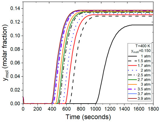
Figure 12.
Results from the FORTRAN program representing the molar fraction of water at the outlet under different conditions.
The test illustrated in Figure 13 was conducted under various operating conditions, specifically with a feed mol fraction of ymol0 = 0.200, representing the water concentration in the binary mixture. Under these conditions, the program calculates that the process reaches bed saturation between 250 and 500 s for pressure ranging from 1.5 to 3.9 atm. The breakthrough curve at atmospheric pressure reaches saturation in 1100 s, extending the time required for the adsorption process to conclude. The behavior observed in Figure 13 aligns with what has been reported in previous studies [7,14,37,46]. Additionally, the time intervals are consistent with those reported in the work by Karmi et al. [13].
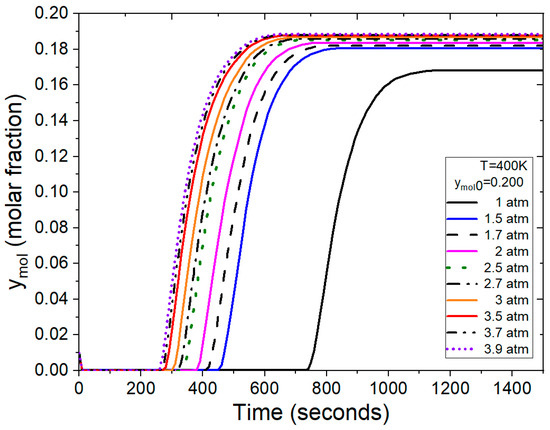
Figure 13.
Breakthrough curves at the outlet of adsorption column at various pressures and temperatures.
Finally, it is important to mention that despite the application of synthetic zeolites in the chemical industry being more widespread, in this paper, the use of natural zeolite clinoptilolite was addressed with the view that its use offers a more cost-effective solution for small-scale bioethanol-producing industries, such as small worker-owned industrial cooperatives in rural areas, which often lack sufficient financial resources to cover the expenses associated with synthetic zeolites. In this regard, the current research provides an alternative for small-scale industries to address the potential variability arising from fluctuations in the composition of the primary mineral characteristic of natural zeolites.
4. Conclusions
The implementation of the Peng–Robinson equation in the PSA model has not only highlighted its impact on numerical solutions but has also contributed to comprehensively expanding water and ethanol datasets across varying pressure and temperature conditions. The observed improvements in calculation accuracy, with reductions in prediction errors by 5–10% compared to the ideal gas law, underscore the significance of employing a more rigorous state equation, particularly at moderate to high pressures and low to moderate temperature. These enhancements are crucial for achieving reliable and accurate predictions of real process dynamics in industrial applications. The improved dataset provides valuable insights into the thermodynamic behavior of ethanol–water mixtures and serves as a foundation for future research. The results from the breakthrough curves and the detailed understanding of the adsorption cycle contribute significantly to refining the PSA process for ethanol dehydration. This study lays the groundwork for future investigations into packed bed regeneration, pressure drop modeling, and mass flow optimization, all of which will further enhance the efficiency and reliability of PSA processes in ethanol dehydration.
Author Contributions
Conceptualization, G.R.U.-G.; data curation, G.L.-S., M.G.A.-U., J.G.-R. and G.R.U.-G.; formal analysis, D.C.-L. and G.R.U.-G.; funding acquisition, G.R.U.-G.; investigation, D.G.-G. and G.R.U.-G.; methodology, D.G.-G., G.L.-S., D.C.-L., M.G.A.-U., J.G.-R. and G.R.U.-G.; project administration, G.R.U.-G.; software, D.G.-G. and G.R.U.-G.; supervision, G.R.U.-G.; validation, M.G.A.-U. and J.G.-R.; visualization, D.G.-G., D.C.-L., M.G.A.-U. and J.G.-R.; writing—original draft, D.G.-G. and G.R.U.-G.; writing—review and editing, G.R.U.-G. All authors have read and agreed to the published version of the manuscript.
Funding
This research was funded by the Consejo Veracruzano de Investigación Científica y Desarrollo Tecnológico (COVEICYDET). Funding number CJ AR 033/2024.
Data Availability Statement
The data supporting the findings of this study are available from the corresponding author, Galo Rafael Urrea-García, upon reasonable request. Simulation data and experimental results have been archived and can be shared for further research purposes.
Acknowledgments
This work was published thanks to the support of the Consejo Veracruzano de Investigación Científica y Desarrollo Tecnológico (COVEICYDET). Funding number CJ AR 033/2024.
Conflicts of Interest
The authors declare no conflicts of interest. The research was conducted without any commercial or financial relationships that could be construed as a potential conflict of interest.
References
- Lee, J.; Cho, H.; Kim, J. Techno-economic analysis of on-site blue hydrogen production based on vacuum pressure adsorption: Practical application to real-world hydrogen refueling stations. J. Environ. Chem. Eng. 2023, 11, 109549. [Google Scholar] [CrossRef]
- Brizuela-Mendoza, J.A.; Sorcia-Vázquez, F.D.J.; Rumbo-Morales, J.Y.; Ortiz-Torres, G.; Torres-Cantero, C.A.; Juárez, M.A.; Zatarain, O.; Ramos-Martinez, M.; Sarmiento-Bustos, E.; Rodríguez-Cerda, J.C.; et al. Pressure Swing Adsorption Plant for the Recovery and Production of Biohydrogen: Optimization and Control. Processes 2023, 11, 2997. [Google Scholar] [CrossRef]
- Takiguchi, Y.; Osada, O.; Uematsu, M. Thermodynamic properties of {xC2H5OH+(1−x)H2O} in the temperature range from 320 K to 420 K at pressures up to 200 MPa. J. Chem. Thermodyn. 1996, 28, 1375–1385. [Google Scholar] [CrossRef]
- Kupiec, K.; Rakoczy, J.; Zieliński, L.; Georgiou, A. Adsorption-Desorption Cycles for the Separation of Vapor-Phase Ethanol/Water Mixtures. Adsorpt. Sci. Technol. 2008, 26, 209–224. [Google Scholar] [CrossRef]
- Küüt, A.; Ritslaid, K.; Küüt, K. Chapter 3—State of the art on the conventional processes for ethanol production. In Ethanol Science and Engineering, 1st ed.; Elsevier: Tartu, Estonia, 2019; pp. 45–68. [Google Scholar] [CrossRef]
- Guevara Luna, M.A.; Fredy Alejandro, F.A.; Belalcazar, L.C. Experimental Data and New Binary Interaction Parameters for Ethanol-Water VLE at Low Pressures Using NRTL and UNIQUAC. Tecciencia 2018, 12, 17–26. [Google Scholar] [CrossRef]
- Kupiec, K.; Rakoczy, J.; Komorowicz, T.; Larwa, B. Heat and Mass Transfer in Adsorption–Desorption Cyclic Process for Ethanol Dehydration. Chem. Eng. J. 2014, 241, 485–494. [Google Scholar] [CrossRef]
- Sinha, P.; Padivar, N. Optimal startup operation of a pressure swing adsorption. IFAC-PapersOnLine 2019, 52, 130–135. [Google Scholar] [CrossRef]
- Geankoplis, C.J.; Lepek, D.H.; Hersel, A. Transport Processes and Separation Process Principles, 5th ed.; Pearson: New York, NY, USA, 2018. [Google Scholar]
- Carmo, M.J.; Gubulin, J.C. Ethanol-Water Separation in the PSA Process. Adsorption 2002, 8, 235–248. [Google Scholar] [CrossRef]
- Simo, M.; Brown, C.J.; Hlavacek, V. Simulation of Pressure Swing Adsorption in Fuel Ethanol Production Process. Comput. Chem. Eng. 2008, 32, 1635–1649. [Google Scholar] [CrossRef]
- Kupiec, K.; Rakoczy, J.; Lalik, E. Modeling of PSA Separation Process Including Friction Pressure Drop in Adsorbent Bed. Chem. Eng. Process. 2009, 48, 1199–1211. [Google Scholar] [CrossRef]
- Saleman, T.L.; Li, G.; Rufford, T.E.; Stanwix, P.L.; Chan, K.I.; Huang, S.H.; May, E.F. Capture of Low-Grade Methane from Nitrogen Gas Using Dual-Reflux Pressure Swing Adsorption. Chem. Eng. J. 2015, 285, 739–748. [Google Scholar] [CrossRef]
- Karimi, S.; Ghobadian, B.; Omidkhah, M.-R.; Towfighi, J.; Yaraki, M.T. Experimental Investigation of Bioethanol Liquid Phase Dehydration Using Natural Clinoptilolite. J. Adv. Res. 2016, 7, 435–444. [Google Scholar] [CrossRef]
- Rossi, E.; Paloni, M.; Storti, G.; Masi, M.; Morbidelli, M. Modeling Dual Reflux-Pressure Swing Adsorption Processes: Numerical Solution Based on the Finite Volume Method. Chem. Eng. Sci. 2019, 203, 173–185. [Google Scholar] [CrossRef]
- Morales, J.Y.R.; López, G.L.; Martínez, V.M.A.; Vázquez, F.d.J.S.; Mendoza, J.A.B.; García, M.M. Parametric Study and Control of a Pressure Swing Adsorption Process to Separate the Water-Ethanol Mixture Under Disturbances. Sep. Purif. Technol. 2019, 236, 116214. [Google Scholar] [CrossRef]
- Pruzan, P.; Ter Minassian, L.; Figuiere, P.; Szwarc, H. High Pressure Calorimetry as Applied to Piezothermal Analysis. Rev. Sci. Instrum. 1976, 47, 66–71. [Google Scholar] [CrossRef]
- Yusa, M.; Mathur, G.P.; Stager, R.A. Viscosity and Compression of Ethanol-Water Mixtures for Pressures up to 40,000 psig. J. Chem. Eng. Data 1977, 22, 32–35. [Google Scholar] [CrossRef]
- Moriyoshi, T.; Inubishi, H. Compression of Some Alcohols and Their Aqueous Binary Mixtures at 298.15 K and at Pressures up to 1400 atm. J. Chem. Thermodyn. 1977, 9, 587–592. [Google Scholar] [CrossRef]
- Gupta, A.C.; Hanks, R.W. Liquid Phase PVT Data for Binary Mixtures of Toluene with Nitroethane and Acetone, and Benzene with Acetonitrile, Nitromethane, and Ethanol. Thermochim. Acta 1977, 21, 143–152. [Google Scholar] [CrossRef]
- Schroeder, J.A.; Penoncello, S.G.; Schroeder, J.S. A Fundamental Equation of State for Ethanol. J. Phys. Chem. Ref. Data 2014, 43, 043102. [Google Scholar] [CrossRef]
- Dillon, H.E.; Penoncello, S.G. A Fundamental Equation for Calculation of the Thermodynamic Properties of Ethanol. Int. J. Thermophys. 2004, 25, 321–335. [Google Scholar] [CrossRef]
- Ozawa, S.; Ooyatsu, N.; Yamabe, M.; Honmo, S.; Ogino, Y. Specific Volumes of Binary Liquid Mixtures at High Pressures. J. Chem. Thermodyn. 1980, 12, 229–242. [Google Scholar] [CrossRef]
- Ortega, J. Densities and Refractive Indices of Pure Alcohols as a Function of Temperature. J. Chem. Eng. Data 1982, 27, 312–317. [Google Scholar] [CrossRef]
- Easteal, A.J.; Woolf, L.A. Measurement of (p, V, x) for (ethanol + trichloromethane) at 298.15 K. J. Chem. Thermodyn. 1984, 16, 391–398. [Google Scholar] [CrossRef]
- Kubota, H.; Tanaka, Y.; Makita, T. Volumetric Behavior of Pure Alcohols and Their Water Mixtures Under High Pressure. Int. J. Thermophys. 1987, 8, 47–70. [Google Scholar] [CrossRef]
- Sun, T.; Schouten, J.; Trappeniers, N.; Biswas, S. Measurements of the Densities of Liquid Benzene, Cyclohexane, Methanol, and Ethanol as Functions of Temperature at 0.1 MPa. J. Chem. Thermodyn. 1988, 20, 1089–1096. [Google Scholar] [CrossRef]
- Sun, T.F.; Schouten, J.A.; Biswas, S.N. Determination of the Thermodynamic Properties of Liquid Ethanol from 193 to 263 K and Up to 280 Mpa from Speed-of-Sound Measurements. Int. J. Thermophys. 1991, 12, 381–395. [Google Scholar] [CrossRef]
- Sun, T.F.; Seldam, C.A.T.; Kortbeek, P.J.; Trappeniers, N.J.; Biswas, S.N. Acoustic and Thermodynamic Properties of Ethanol from 273.15 to 333.15 K and Up to 280 MPa. Phys. Chem. Liq. 1988, 18, 107–116. [Google Scholar] [CrossRef]
- Sun, T.F.; Schouten, J.A.; Kortbeek, P.J.; Biswas, S.N. Experimental Equations of State for Some Organic Liquids Between 273 and 333 K and Up to 280 MPa. Phys. Chem. Liq. 1990, 21, 231–237. [Google Scholar] [CrossRef]
- Hales, J.L.; Ellender, J.H. Liquid Densities from 293 to 490 K of Nine Aliphatic Alcohols. J. Chem. Thermodyn. 1976, 8, 1177–1184. [Google Scholar] [CrossRef]
- Takiguchi, Y.; Uematsu, M. PVT Measurements of Liquid Ethanol in the Temperature Range from 310 to 363 K at Pressures up to 200 MPa. Int. J. Thermophys. 1995, 16, 205–214. [Google Scholar] [CrossRef]
- Takiguchi, Y.; Uematsu, M. Densities for Liquid Ethanol in the Temperature Range from 310 to 480 K at Pressures up to 200 MPa. J. Chem. Thermodyn. 1996, 28, 7–16. [Google Scholar] [CrossRef]
- Mousa, A.H.N. Critical Properties, Heat of Vaporization, and Vapour Pressure of Ethanol from 20 kPa to the Critical Point. J. Chem. Eng. Jpn. 1987, 20, 635–637. [Google Scholar] [CrossRef][Green Version]
- Bazaev, A.R.; Abdulagatov, I.M.; Bazaev, E.A.; Abdurashidova, A. PVT Measurements for Pure Ethanol in the Near-Critical and Supercritical Regions. Int. J. Thermophys. 2007, 28, 194–219. [Google Scholar] [CrossRef]
- Polikhronidi, N.; Abdulagatov, I.; Stepanov, G.; Batyrova, R. Isochoric Heat Capacity Measurements for Pure Ethanol in the Near-Critical and Supercritical Regions. J. Supercrit. Fluids 2007, 43, 1–24. [Google Scholar] [CrossRef]
- Fotouh, K.; Shukla, K. An Improved Peng-Robinson Equation of State with a New Temperature-Dependent Attractive Term. Chem. Eng. Commun. 1997, 159, 209–229. [Google Scholar] [CrossRef]
- Peng, D.Y.; Robinson, D.B. A New Two-Constant Equation of State. Ind. Eng. Chem. Fundam. 1976, 15, 59–64. [Google Scholar] [CrossRef]
- Gao, G.; Daridon, J.-L.; Saint-Guirons, H.; Xans, P.; Montel, F. A Simple Correlation to Evaluate Binary Interaction Parameters of the Peng-Robinson Equation of State: Binary Light Hydrocarbon Systems. Fluid Phase Equilibria 1992, 74, 85–93. [Google Scholar] [CrossRef]
- Gutiérrez-González, D.; Urrea-García, G.; Luna-Solano, G.; Cantú-Lozano, D.; Gómez-Rodriguez, J. Numerical Solution of Adsorption Cycle in Ethanol Dehydration Process. Procedia Manuf. 2020, 49, 32–37. [Google Scholar] [CrossRef]
- Wilson, K.S.; Lindley, D.D.; Kay, W.B.; Abraham, R.J. Virial Coefficients of Ethanol from 373.07 to 473.15 K. J. Chem. Eng. Data 1984, 29, 243–245. [Google Scholar] [CrossRef]
- Smith, J.M.; Van Ness, H.C.; Abbott, M.M.; Swihart, M.T. Introduction to Chemical Engineering Thermodynamics, 8th ed.; McGraw-Hill Education: New York, NY, USA, 2018. [Google Scholar]
- Chapra, S.C.; Canale, R.P. Numerical Methods for Engineers, 6th ed.; McGraw-Hill: New York, NY, USA, 2010. [Google Scholar]
- Cengel, Y.A.; Boles, M.A. Thermodynamics: An Engineering Approach, 7th ed.; McGraw-Hill: New York, NY, USA, 2011. [Google Scholar]
- International Association for the Properties of Water and Steam (IAPWS). Available online: http://www.iapws.org (accessed on 20 August 2024).
- Leo-Avelino, G.; Urrea-García, G.R.; Gómez-Rodríguez, J.; Torres-Pazmiño, R.A.; Rumbo-Morales, J.Y. Natural Mexican Clinoptilolite for Ethanol Dehydration: Adsorption–Regeneration Experimental Parameter Determination and Scaling–Up at Pilot Plant. Rev. Mex. Ing. Quím. 2021, 20, 1367–1379. [Google Scholar] [CrossRef]


Disclaimer/Publisher’s Note: The statements, opinions and data contained in all publications are solely those of the individual author(s) and contributor(s) and not of MDPI and/or the editor(s). MDPI and/or the editor(s) disclaim responsibility for any injury to people or property resulting from any ideas, methods, instructions or products referred to in the content. |
© 2025 by the authors. Licensee MDPI, Basel, Switzerland. This article is an open access article distributed under the terms and conditions of the Creative Commons Attribution (CC BY) license (https://creativecommons.org/licenses/by/4.0/).