Pressure Relief-Type Overpressure Prediction in Sand Body Based on BP Neural Network

Abstract

With the gradual depletion of global oil and gas resources, accurate prediction of anomaly formation pressure caused by pressure relief from other sources has become increasingly crucial in oil and gas exploration and development. The anomaly formation pressure caused by pressure relief affects the well’s stability and significantly impacts the safety and economy of drilling operations. However, traditional methods for predicting anomaly formation pressure, such as Bowers’ method, may not accurately identify the complex relationship between parameters and pore pressure. In contrast, the BP neural network (BPNN) can learn the complex relationship between input and output from data, which has a significant advantage in accurately identifying anomaly formation pressures caused by pressure relief from other sources. This study proposes a neural network-based method for accurately predicting anomaly formation pressure caused by pressure relief from other sources. The high quality of input data is ensured through meticulous preprocessing related to anomaly formation pressure caused by pressure relief from other sources, including data cleaning, standardization, and correlation analysis. Subsequently, model training was conducted to fully utilize its powerful nonlinear fitting ability and capture the complex changes in formation pressure caused by anomaly pressure relief from other sources. This method collects and organizes the parameters of the formation, including Gamma-ray (Gr), Delta-T (Dt), wave velocity (V_p), and Resistivity (R10), to train a BPNN model for predicting pressure relief type anomaly formations. The trained model has a Bayesian regularized backpropagation function, and the average absolute percentage error (AAPE) and correlation coefficient (R) of predicting pore pressure in well A are 4.22% and 0.875, respectively. To verify the proposed model’s effectiveness, it was applied to a blind dataset of adjacent B wells and successfully predicted pore pressure with AAPE of 5.44% and R of 0.864. We compare and analyze the formation pore pressure predicted by the traditional Bowers model and support vector machine (SVM) model. The prediction results of the BPNN model have more minor errors and are closer to the actual pressure coefficient. This study demonstrates the accuracy of the proposed model in predicting pressure relief type anomaly formation pressure using drilling data.

1. Introduction

Formation pressure, also known as pore pressure, refers to the pressure exerted by fluids within the pore space of a formation. This pressure is crucial in all aspects of drilling and gas well completion. It affects the selection of drilling rigs, the design of drilling mud, casing, and cementing procedures, and the overall completion plan. Understanding and accurately assessing formation pressure is crucial for ensuring drilling operations’ safety, efficiency, and integrity and mitigating wellbore stability and integrity risks. Therefore, the fundamental parameter guides decision making in the entire drilling and completion process [1,2].

The underground pore pressure state is not constant but is influenced by factors such as pore fluid, formation permeability, stress, sedimentation rate, and temperature. After a certain period, the pore pressure will be higher or lower than usual, forming anomaly high or anomaly low pressure. The formation mechanisms of abnormally high pressure are diverse, and the superposition of multiple formation mechanisms may generate the anomaly pressure of a formation, and one of them may dominate [3]. The currently publicly available mechanisms for the formation of abnormally high pressure include compaction, tectonic processes (including tectonic compression, stratigraphic uplift, diapir, folding, faulting, landslides, collapses, and punctures), water head effects, buoyancy effects (also known as density differences), fluid migration, permeation, hydrothermal pressurization, mineral transformation, and hydrocarbon generation (including hydrocarbon generation and thermal cracking of liquid hydrocarbons) [4,5,6].

There are multiple criteria for classifying anomaly formation pressure. To meet the principle of facilitating an accurate description of overpressure, Li Wei defines a pressure coefficient less than 0.9 as a low-pressure anomaly, 0.9–1.2 as normal formation pressure, 1.2–1.6 as weak anomaly high pressure, and 1.6–2 as intense anomaly high pressure [7]. The Chinese petroleum industry standard defines a pressure coefficient less than 0.9 as a low-pressure gas reservoir, 0.9~1.3 as a normal-pressure gas reservoir, 1.3~1.8 as a high-pressure gas reservoir, and greater than 1.8 as an ultra-high-pressure gas reservoir [8]. According to petroleum geological theory and oil and gas exploration practice, formations with a pressure coefficient less than 0.75 are generally defined as ultra-low-pressure formations, 0.75–0.9 as low-pressure formations, 0.9–1.1 as normal-pressure formations, 1.1–1.4 as high-pressure formations, and greater than 1.4 as ultra-high-pressure formations [9]. When the formation pressure is lower than normal, it may cause differential pressure sticking and mud leakage. On the other hand, excessive pressure may lead to pressure surges and blowouts during drilling operations. Geological, mechanical, geochemical, geothermal factors or a combination may cause overpressure. These complications not only disrupt the execution of the project but also increase costs and, in the worst case, can cause serious health and safety hazards. Real-time pore pressure prediction can improve wellbore trajectory, casing, and mud program design and provide better wellbore stability analysis, thereby saving drilling time and costs [10,11,12,13].

Several methods for predicting pore pressure have been developed, including empirical, analytical, and numerical methods [2,14,15,16]. The empirical method is based on the correlation calculation between pore pressure and other logging data, such as sound velocity, porosity, and resistivity logging. These methods are widely used in industry due to their simplicity and ease of use. However, empirical methods have limitations, especially when the correlation is based on a limited dataset and when the geological environment differs from the geological environment used for developing the correlation. That requires modifying the original model parameters for the new geological structure [17]. In addition to traditional methods, Xu Baorong et al. proposed a matching technique for predicting formation pressure based on the seismic layer velocity method, characteristic curve inversion method, and improved Fillippone formula [18]. In 2018, Kiss et al. constructed a multi-input–output neural network and used 139 fracturing construction data to establish a neural network model for predicting formation fracture pressure [19]. Qian Liping et al. used the equivalent medium theory elastic modulus boundary algorithm, combined with well seismic joint inversion, to achieve formation pressure prediction [20]. Wang et al. used indoor component simulation results as training data and proposed a flash evaporation calculation model using neural networks to accelerate component modelling [21]. This model is used to predict the saturation pressure at a given component and pressure and to determine phase stability by comparing the predicted pressure with the system pressure. Li Yufeng et al. established an identification factor for anomaly formation pressure based on logging response characteristics and pre-stack elastic wave impedance inversion, achieving formation pressure prediction [22].

In recent years, artificial intelligence technology has developed rapidly both domestically and internationally and has significant advantages in solving complex nonlinear problems. It has also begun to be applied and developed in exploration and evaluation [23,24], reservoir description [25,26], production prediction [27,28], and development optimization [29,30] in the petroleum field. In terms of performance evaluation in stress prediction, BP neural networks and deep learning methods have also made significant progress [31,32,33,34,35,36].

Artificial intelligence technology is gradually showing advantages in predicting formation pressure. Primasty used the equivalent depth method to analyze the depth of anomaly pore pressure in Nova Scotia, Canada [2]. Abdulmalek et al. used drilling parameters and machine learning algorithms to predict formation pore pressure [37]. Hadi et al. used artificial neural networks to predict formation pressure based on seismic and reservoir parameters [38]. Rashidi et al. also used neural networks to predict elastic modulus [39] and formation pore pressure [40].

The purpose of this study is to establish a prediction model of anomaly formation pore pressure of pressure relief type based on well-logging data such as Gama (Gr), interval propagation time (Dt), wave velocity, and resistivity (R10), combined with BP neural network algorithm, to predict the pressure relief type anomaly formation pore pressure. In the first part of this article, the data are partitioned, and the processed data are divided into pressure relief data and pressure rise data. The abnormally high-pressure relief section data are used to train a BP neural network model. Subsequently, the pressure rise data are used as input data for prediction, and the pressure rise data from another well are used for prediction. The error and correlation coefficient are compared between the predicted anomaly pressure value and the actual pressure values of the two wells. In the second part of this article, the steps for establishing a prediction of anomaly formation pore pressure are explained. The third part of this article uses a trained Bayesian regularized backpropagation function model to predict anomaly pore pressure in well A, with an average absolute percentage error (AAPE) and correlation coefficient (R) of 4.22% and 0.875, respectively. To verify the proposed correlation, it was applied to a blind dataset of another adjacent B well, and the model successfully predicted anomaly pore pressure with an AAPE of 5.44% and an R of 0.864.

This proposed method for predicting anomaly formation pore pressure is of great significance, especially when other methods for predicting anomaly formation pore pressure are not feasible. Utilizing the BP neural network provides a novel and potentially more effective method for predicting anomaly formation pore pressure, which utilizes the BP neural network to identify complex correlations in complex datasets. This study has made valuable contributions to predicting anomaly formation pore pressure, proposing a feasible alternative solution that helps improve accuracy and reliability. It can modify various drilling parameters during the drilling process on time and reduce accidents, especially when traditional methods cannot meet the requirements in specific geological environments.

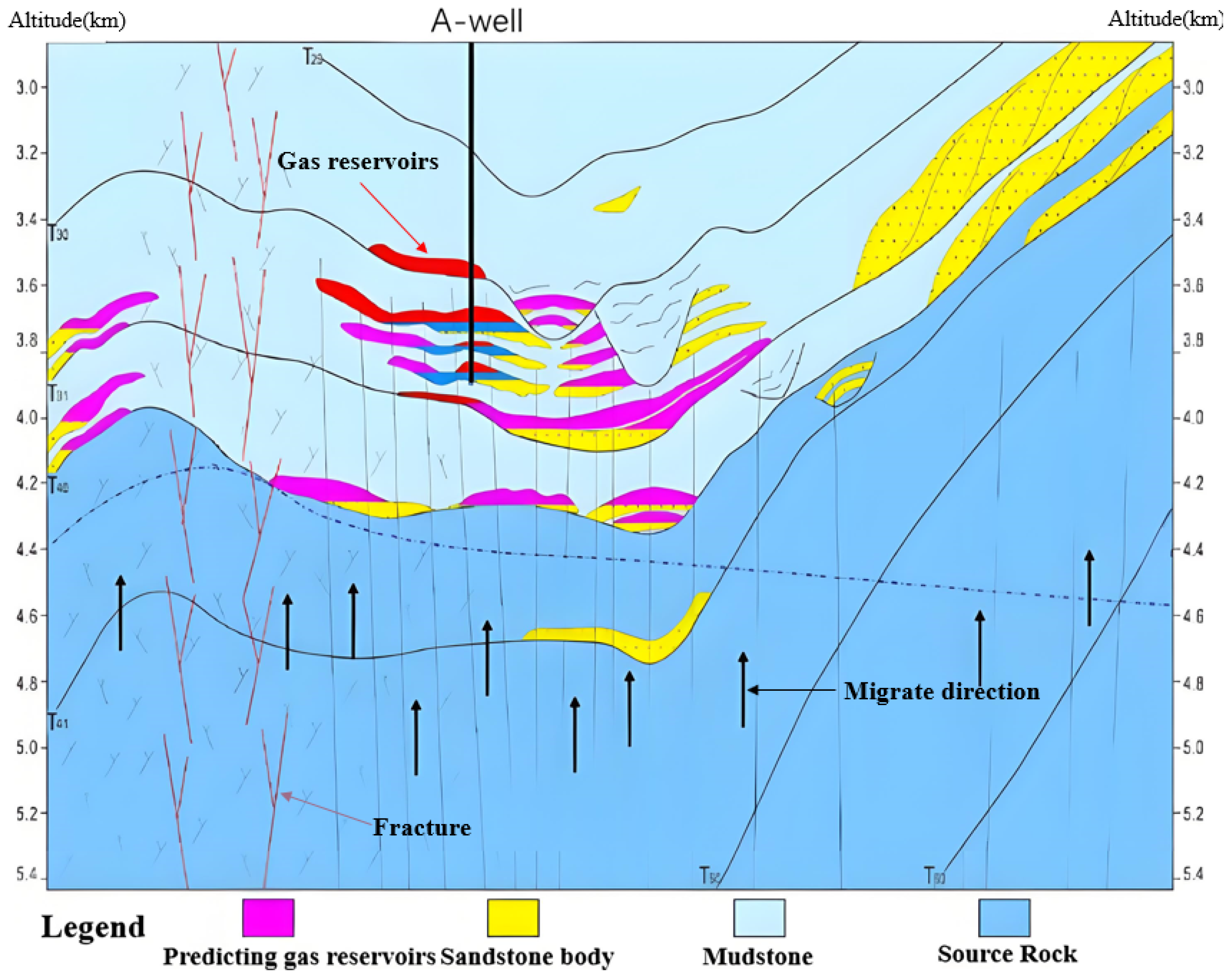
2. Anomaly Formation Pressure of Other Source Relief Type

At present, there are three main classification methods for abnormally high pressure [41]: based on the source of action (self-source, external source), based on volume change (fluid volume change, pore volume change, and fluid pressure change with fluid motion), and based on the mechanical relationships during the original sedimentation process (loading, unloading, and porosity remain unchanged).

The mechanism of abnormally high-pressure formation is mainly determined based on qualitative judgments such as sedimentary structural history, reservoir properties, and oil and gas generation conditions. Later, as the study of mechanical relationships during rock deposition continued to deepen, methods for determining the anomaly high-pressure pressure mechanism using logging data were developed, including the acoustic density intersection plot method, the acoustic effective stress intersection plot method, and the acoustic resistivity density curve method.

This study’s lateral pressure relief process of sandstone reservoirs belongs to overpressure migration. Fluid migration and dissipation can cause changes in pressure, and without pressurization, it can lead to a decrease in overpressure. Therefore, it is an essential factor in controlling the distribution and evolution of overpressure. The faults in the well area are not well developed. Still, delta sand bodies are deposited, which serve as channels for pressure release and can affect the well area’s pressure distribution and evolution characteristics. When the fault system is not developed, but the high-pressure formation is in direct contact with the overlying large sedimentary body, pressure relief can also occur. This pressure of relief type requires good lateral connectivity, a wide distribution range, and an upward connection with the hydrostatic pressure system of the sizeable sedimentary body. The continuous distribution of sedimentary bodies corresponds to normal or transitional pressure zones. In contrast, isolated sand bodies or areas without developed sedimentary bodies correspond to higher pressure coefficients, indicating that widely distributed sedimentary sand bodies are channels for overpressure release. Stratigraphic pressure relief is often the result of the combined action of multiple geological factors, such as the opening and closing of faults, the generation of fracture zones caused by bottom fissures, and so on. The power for pressure relief comes from the pressure difference between a high-pressure source and a low-pressure source (such as hydrostatic pressure). The influence of induced or high-permeability fractures on pressure relief is also significant, and the pressure relief channel is a high-permeability connected sand body. The result of pressure relief is a redistribution of pressure within a specific range around the relief channel. The pressure relief layer of a high permeability sand body is necessary for achieving lateral pressure relief of reservoirs. It is the main controlling factor affecting the direction and distance of lateral pressure relief.

A well encountered two types of pressure relief formations (single sand body pressure relief and overall formation pressure relief), with a wide distribution of sand bodies. One wing extends to the slope zone, while the other wing connects to the bottom splitting structure, providing good pressure relief conditions. The use of mud with high density during drilling pollutes the reservoir. Therefore, it is crucial to accurately predict the anomaly formation pressure of relief type in the region (Figure 1 and Figure 2).

3. Materials and Methods

3.1. Traditional Model—Bowers Method

(1)

Establishment of Bowers method detection model

Bowers proposed this method in 1995 [42]. He systematically considered the under-compaction of shale and other compaction mechanisms besides under-compaction. The Bowers method is based on the effective stress theorem. It directly calculates the vertical effective stress using the original loading and unloading curve equations (The loading curve can be obtained by integrating the established normal compacted formation density along the well depth and subtracting the normal pore pressure. According to the principle of equivalent depth, this curve is also the characteristic curve of loading overpressure. Bowers’ unloading equation is traditionally used for the unloading curve, but it shows that the deep rock has entered a plastic state, and the stress of the rock skeleton is unloaded due to fluid expansion and pressurization, basically without deformation recovery, and the density is basically unchanged.) between the vertical effect force and the acoustic velocity. Combined with the overlying rock pressure, the formation pore pressure can be obtained, so there is no need to establish a normal trend line.

Original loading curve of shale:

$$V=V_0+A{{\sigma }_{ev}}^B$$

(1)

In the formula, V is the wave velocity, ft/s; ${\sigma }_{ev}$ is the vertical effective stress (obtained from measured formation pressure or normal compaction section data); V₀ and B are model parameters obtained through regression analysis of neighboring well data (V, ${\sigma }_{ev}$).

Unloading curve equation:

$$V=V_0+A{\left[{\sigma }_{\max }{\left(\sigma /{\sigma }_{\max }\right)}^{1/U}\right]}^B$$

(2)

The ‘${\sigma }_{\max }$’ in the formula is determined by the following equation:

$${\sigma }_{\max }={\left({\displaystyle \frac{V_{\max }-V_0}{A}}\right)}^{1/B}$$

(3)

In the formula, ${\sigma }_{max}, V_{max}$ are the maximum vertical effective stress and acoustic velocity at the beginning of unloading; U is the elastic–plastic coefficient of shale.

In formations where mudstone unloading is caused by fluid expansion, the decrease in acoustic velocity is more pronounced compared to under-compaction, which Bowers refers to as velocity reversal (Under normal circumstances, the acoustic wave velocity (or seismic wave velocity) of a formation increases with depth, as deep formations are typically denser. However, in some cases, the velocity decreases with increasing depth, a phenomenon known as velocity reversal). In these formations, high pressure caused by fluid expansion dominates, and the vertical effective stress is determined using the unloading curve equation. In other formations, the original loading curve equation determines the stress.

(2)

Determination of Model Parameters

Regarding the determination of ${\sigma }_{max}$ and $V_{max}$, In the case of little change in lithology, $V_{max}$ is usually taken as the velocity value at the beginning of the reversal. At this point, it is assumed that the rocks within a certain thickness of the inversion zone have experienced the same maximum stress state at the same time in the past.

Regarding the elastic–plastic coefficient U, U = 1 indicates no permanent deformation and complete elasticity, and the unloading curve coincides with the loading curve. U = ∞ represents completely irreversible deformation and is completely plastic. For the mudstone encountered during drilling, the range of U value variation is generally 3–8, with little difference within the same area.

The determination of the U value is more complex than the determination of A and B values, because the unloading curve data ($P_p$, $P_o$, ${\sigma }_{ev}$, $V$, ${ V}_{max}$, ${ \sigma }_{max}$, etc.) of the same formation obtained from different wells in the region are on different unloading curves because even if the lithology is not significantly different, the maximum stress state experienced by the formation may also be different. Using multi-well data to obtain the U value, the following method is used to standardize the data.

$$({\sigma }_{ev}/{\sigma }_{\max })={({\sigma }_{vc}/{\sigma }_{\max })}^U$$

(4)

In the formula, ${\sigma }_{vc}=\left[\right(V-5000)/A{]}^{({\displaystyle \frac{1}{B}})}$, substitute the velocity value of a specific point on the unloading curve with the vertical effective stress value calculated by the loading equation.

(3)

Characteristics of the method

The Bowers method uses unloading curves to describe the abnormally high pressure caused by the expansion of pore fluids, which improves the calculation accuracy of the abnormally high pressure caused by the fluid expansion mechanism. That is a breakthrough in the method of determining formation pore pressure.

3.2. Traditional Model—Eaton Method

(1)

Model Introduction

The Eaton method [43] is commonly used to calculate formation pore pressure in domestic and foreign oilfield companies. It has the characteristics of high calculation accuracy and wide application range. The theoretical basis of this method is the theory of under-compaction.

This method can use acoustic time difference, resistivity, density, and Dc index data to calculate formation pressure. The Eaton method calculates the pattern of formation pore pressure gradient as follows:

$$P_p=P_{ob}-(P_{ob}-P_h){\left({\displaystyle \frac{\Delta t_n}{\Delta t_o}}\right)}^N$$

(5)

$$P_p=P_{ob}-(P_{ob}-P_h){\left({\displaystyle \frac{R_o}{R_n}}\right)}^N$$

(6)

$$P_p=P_{ob}-(P_{ob}-P_h){\left({\displaystyle \frac{D_e}{D_{en}}}\right)}^N$$

(7)

$$P_p=P_{ob}-(P_{ob}-P_h){\left({\displaystyle \frac{D_e}{D_{en}}}\right)}^N$$

(8)

$$P_p=P_{ob}-(P_{ob}-P_h){\left({\displaystyle \frac{d_c}{d_{cn}}}\right)}^N$$

(9)

In the formula, $P_p$ is the pore pressure of the formation; $P_{ob}$ is the overlying rock pressure; $P_h$ is the normal hydrostatic pressure; $\Delta t_n$, $R_n$, $D_{en}$, $d_{cn}$ are the usual trend line acoustic time difference, resistivity, density, and Dc index values of shale at a certain depth, while $\Delta t_o$, $R_o$, $D_e$, and $d_c$ are the measured acoustic time difference, resistivity, density, and Dc index values of shale formations at a given depth; N is the Eaton index, a coefficient related to geological formations.

(2)

Normal compaction trend line

There is a proportional relationship between acoustic time difference and porosity for geological profiles with known lithology and little change in formation water properties. In typically compacted formations, the formula following can be derived:

$$\Delta t_n=\Delta t_0{e}^{AH}$$

(10)

By transforming the above equation, we can obtain:

$$\ln \Delta t_n=AH+B$$

(11)

In the formula, $\Delta t_n$ is the interval transit time of formation at depth H, $\mu s/ft$; $\Delta t_0$ is the interval transit time of formation at depth H, $\mu s/ft$.

This formula is the usual trend line formula for the acoustic time difference of compacted strata. It can be intuitively seen from the formula that there is a linear relationship between $\ln \Delta t$ and H, with a slope of A(A < 0). On the semi-logarithmic curve, the logarithmic value of $\Delta t$ of a customarily compacted formation decreases linearly with depth. If anomaly high pressure occurs, $\Delta t$ scatter point will deviate significantly from the usual trend line.

The standard compaction trend line equations for resistivity, density, and Dc index are in the same form as the standard compaction trend line equation for acoustic time difference. The difference is that slope A < 0 of the standard compaction trend line equation for acoustic time difference differs from slope A > 0 for resistivity, density, and Dc index.

3.3. Neural Network Prediction Method

(1)

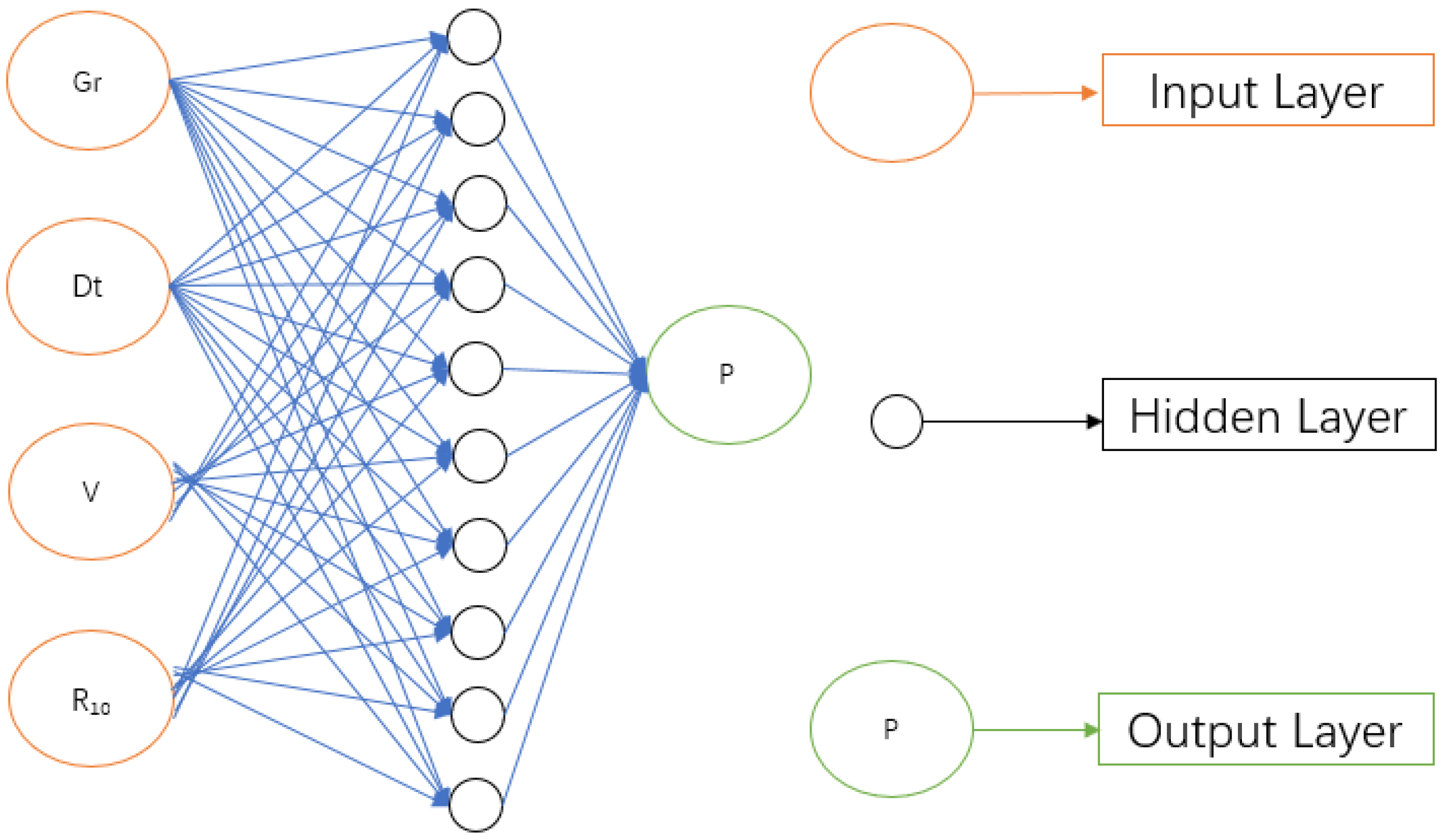
Establishment of Neural Network Model

The BP neural network used in this study is an algorithmic model that mimics the behavioral characteristics of animal neural networks for distributed parallel information processing. This type of network relies on the system’s complexity to process information by adjusting the interconnected relationships between many internal nodes. A classic neural network typically consists of three layers: an input layer, an output layer, and an intermediate layer (also known as a hidden layer). Each layer has multiple node-weighted connections, and input data output is calculated through forward propagation. Then, it undergoes linear transformation and nonlinear processing through hidden layers and activation functions, and finally, the predicted results are outputted through the output layer. Then, iterate and randomly select a batch of training data from the training set, feed this batch of data into the model, and calculate the model’s predicted values. Compare the model’s predicted and actual values and calculate the loss function (loss). Using the cross-entropy function as the loss function, calculate the derivative of the loss function concerning the model variables, pass the obtained derivative values into the optimizer, update the model parameters using the optimizer, and obtain the minimum loss function to minimize errors. The model is successfully established when the minimization loss function reaches its optimum. The mathematical expression formula for neural network data processing (forward propagation) is as follows:

$$y=f(\sum _{i=1}^n w_i{x}_i-b)$$

(12)

In the formula, y represents the output of the neuron; f is the activation function; n is the dimension of the input signal; W_i is the weight of neurons; X_i is the input signal; b is the threshold for neurons. The input signal x_i is weighted by weight w_i and enters the neuron to calculate the total input, compared with the threshold b. Finally, the activation function f is used for nonlinear transformation to generate the total output of the neuron.

The core steps of a BP neural network are as follows (Figure 3). The solid line represents forward propagation, and the dashed line represents backward propagation.

In forward propagation, there is often a step where the output result is compared with the expected result to determine if it meets the requirements. During this process, there will be an error between the actual and expected output results. There is always an objective function: the loss function to reduce this error,

$$\mathrm{L}\mathrm{o}\mathrm{s}\mathrm{s}={\displaystyle \frac{1}{2}}\sum _{i=1}^n{\left(y_i-{\widehat{y}}_i\right)}^2={\displaystyle \frac{1}{2}}\sum _{i=1}{\left[y_i-f\left(W_i{X}_i+b\right)\right]}^2$$

(13)

In the formula, y represents the output result of the neuron; ${\widehat{y}}_i$ is the actual output result; $W_i$ is the weight of neurons; $X_i$ is the input signal; b is the threshold for neurons.

Finding the minimum value of this function is necessary to minimize the error between the actual output result and the expected output result. The general method for finding the minimum value of a function is iteration, which involves finding a numerical solution through gradient descent and iteration. The iterative method generally requires multiple iterations, as the search for the minimum value of the function may require multiple iterations. In each iteration, the weights between nodes in each layer will also be continuously updated.

$$W_{t+1}=W_t-\eta {\displaystyle \frac{\vartheta Loss}{\vartheta W}}+\alpha \left(W_t-W_{t-1}\right)$$

(14)

In the formula, $\eta {\displaystyle \frac{\vartheta Loss}{\vartheta W}}$ is the adjustment amount; $\alpha \left(W_t-W_{t-1}\right)$ is the smoothing term.

Each iteration will generate a weight update, and then the updated weights will be propagated forward with the training samples. If the results are not satisfactory, backpropagation will be performed to continue the iteration. Repeat this process until satisfactory results are obtained.

The activation function used in neural networks is the sigmoid function.

$$\delta \left(x\right)={\displaystyle \frac{1}{1+e^{-x}}}$$

(15)

Evaluate the developed model by determining two statistical parameters: correlation coefficient (R) and mean absolute percentage error (MAPE). R and AAPE are calculated as follows [44]:

$$\mathrm{R}={\displaystyle \frac{N(\sum _1^N Y_i{\widehat{Y}}_i)-(\sum _1^N Y_i)(\sum _1^N \widehat{Y})}{\sqrt{[N\sum _1^N Y_i^2-(\sum _1^N Y_i{)}^2][n\sum _1^N {\widehat{Y}}_i^2-(\sum _1^N {\widehat{Y}}_i{)}^2]}}}$$

(16)

$$\mathrm{A}\mathrm{A}\mathrm{P}\mathrm{E}=\left({\displaystyle \frac{1}{N}}\sum _{i=1}^{\mathrm{N}} \left|{\displaystyle \frac{Y_i-{\widehat{Y}}_i}{Y_i}}\right|\right)\times 100$$

(17)

where N is the number of data points in the dataset, and Y_i is the predicted output.

The model structure’s design is paramount in the modelling process. Usually, the mapping between input and output can be achieved by designing a three-layer architecture (input, hidden, and output) of any continuous function in BPNN [45]. Therefore, this article adopts a three-layer structure of neural networks to establish the model. The input neurons are data corresponding to four parameters: GR, DT, velocity, and R10. Select the measured formation pressure coefficient as the output neuron. In the BP neural network structure, weights and biases connect layers and affect network performance. Many researchers have studied extracting empirical correlations from BPNN structures for more straightforward applications in the petroleum industry by testing several parameters to examine the impact of the number of hidden layers, neurons, network structure, training, and transfer functions on the accuracy of the BPNN model. Figure 4 shows the design of the BPNN model developed in this study.

(2)

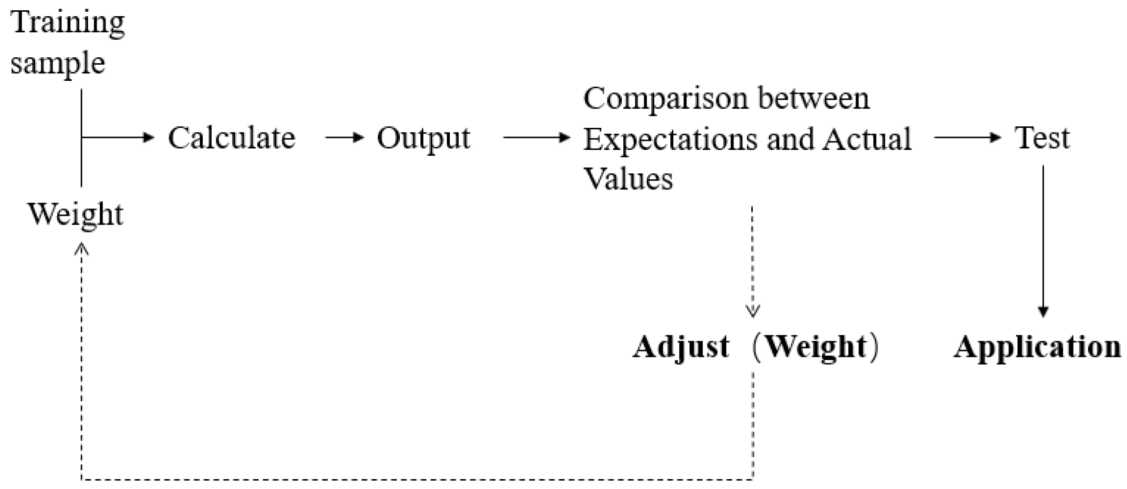
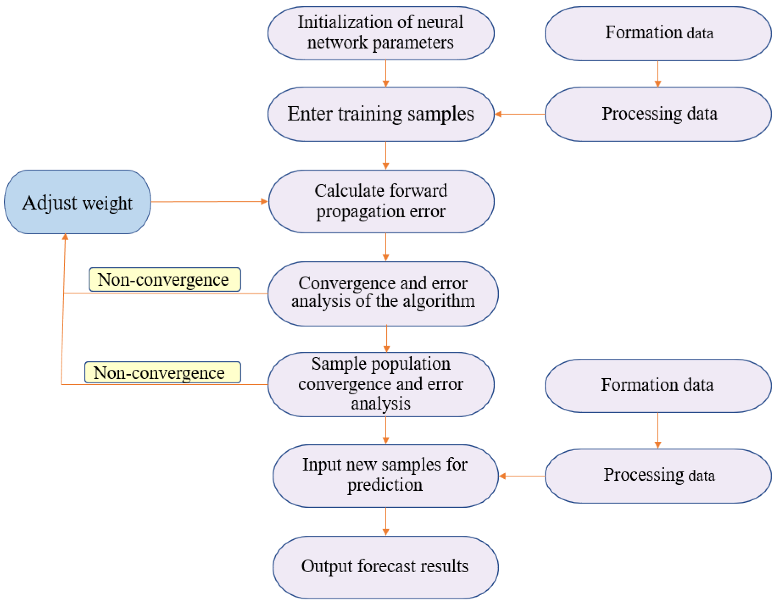
Neural Network Workflow

To predict anomaly formation pressure of relief type, we first collected a large amount of relevant data, such as formation parameters, production data, pressure records, etc. Then, we perform data processing and feature selection, including filling in missing values, normalizing the data, and conducting correlation analysis. On this basis, a neural network-based prediction model was designed, and its parameters were optimized. We adjust the model’s parameters by selecting a suitable neural network structure, including the input, hidden, and output layers. We use appropriate activation functions and optimization algorithms to achieve the optimal solution. The prediction workflow includes the following steps (Figure 5).

(3)

The Limitations of Using BPNNs

Although backpropagation neural networks (BPNNs) perform well in many tasks, they also have some inherent limitations. Understanding these limitations can help to better design, train, and optimize models in practical applications.

1. Overfitting risk

BPNNs have strong fitting ability; especially when the network structure is complex (such as multiple layers and a large number of neurons), the model is prone to overfitting the training data. Overfitting can cause the model to perform well on the training set but poorly on unseen test data. This issue is particularly prominent when training data are limited. In this model, we used regularization techniques to limit the size of weights. At the same time, a Dropout layer is introduced to randomly discard some neurons to reduce overfitting.

2. Sensitivity to hyperparameter adjustment

The performance of BPNN is highly dependent on the selection of hyperparameters, including learning rate, network layers, number of neurons per layer, activation function type, batch size, etc. Inappropriate hyperparameters may lead to slow training, difficult model convergence, or poor performance. We use automated hyperparameter optimization tools such as Bayesian optimization, correlation heatmaps, etc., to select appropriate parameters.

3. Gradient vanishing problem

In deep networks, BPNN may encounter gradient vanishing or gradient exploding problems. The disappearance of gradients can cause slow weight updates in the network and almost halt the training process. Relieve the gradient vanishing problem by using activation functions such as sigmoid.

4. Local optimal solution

The loss function of BPNN is usually non-convex and may have multiple local optima. The training process may converge to suboptimal solutions, resulting in poor model performance. We choose to use random initialization weights and train the model multiple times.

4. Data Processing and Application Analysis

The data used in this article are field data provided by a domestic oil field, including more than 10 types of parameters, such as logging parameters and logging parameters. The raw data from drilling, logging, and logging usually contain many outliers and missing values, which can significantly impact the model’s training effectiveness and computational efficiency. Therefore, reasonable data processing is crucial for artificial intelligence models, as it can improve the model’s quality and reduce its computation time. Use MATLAB (R2022a) software to perform operations such as outlier removal, data completion, and well-logging data partitioning to ensure the accuracy of the formation pore pressure calculation model. The data obtained by correcting the pressure profile using measured values are the actual value of anomaly formation pore pressure, with a relative error of only about 2% compared to the measured points. Finally, an anomaly formation pore pressure sample dataset that can be used for training is established. Next, select the initial model parameters for the first run, update the parameters, and repeat the process until the best results are obtained. Once the optimal outcome is obtained, extract the hyperparameters of the model. Finally, the model was validated using a dataset that did not participate in developing the prediction model.

4.1. Data Cleaning

To accurately predict anomaly formation pore pressure of relief type, data containing approximately 1088 points were collected from the vertical profile of well A in the study area. This set of data parameters includes Gamma-ray (Gr), Delta-T (Dt), wave velocity (V_p), and Resistivity (R10). Due to the physical relationship between Gamma-ray (Gr), acoustic time difference (Dt), wave velocity, resistivity (R10), and pore pressure, they were considered in this work. The gamma value usually refers to the gamma-ray measurement value of the formation, which has a particular relationship with the pore pressure of the formation, inferring some indirect information through gamma values. For example, high gamma values may be associated with high porosity and low-strength formations, leading to higher pore pressure. In oil and gas field development, predicting formation pressure can help determine safe drilling and extraction strategies. Gamma-ray logging data are commonly used to evaluate the behavior of underground fluids and indirectly calculate pore pressure. By measuring DT values and combining them with other data, the pore pressure of the formation can be effectively estimated and analyzed, providing a basis for engineering decisions. By monitoring changes in wave velocity, changes in pore pressure can be indirectly determined, thereby evaluating the stability of the formation, especially during drilling and mining processes. The increase in pore pressure may affect electrical resistivity. As the pore pressure increases, the effective stress of the rock decreases, and the fluidity of the fluid in the pores increases, which may lead to changes in electrical resistivity. By utilizing these physical relationships, artificial neural network models can effectively learn and capture the complex nonlinear interactions between these variables to accurately predict pore pressure in underground formations.

Before training artificial neural network models, preprocessing is performed, which involves filtering out irregular values, such as individual parameter values suddenly increasing or decreasing within a specific depth range, which is considered invalid. Subsequently, the secondary preprocessing step is aimed at removing discrete values. Determine the discrete value based on the statistical distribution of the dataset, and values exceeding ±4.0 standard deviation are considered discrete values. Remove those discrete values from the dataset that may indicate errors or anomalies to ensure the reliability and integrity of the input data. The dataset has been optimized through these preprocessing measures, thereby improving the accuracy of subsequent pore pressure predictions. The prediction error of all input parameters is less than 5%. By ensuring the quality of input through preprocessing, the model’s effectiveness in predicting pore pressure data is improved, minimizing the risk of inaccuracy and distortion, thereby enhancing the model’s ability to make reliable predictions. These predictions are crucial for intelligent decision making in drilling and reservoir engineering applications. Perform statistical analysis on the cleaned data to display each parameter’s minimum, maximum, mean, and standard deviation (

Table 1. Data statistical analysis.

Statistical Parameter	Depth (m)	Gr (dpi)	Dt (μs/ft)	Vp (km/s)	R10 (Ω·m)	Pressure Coefficient
Maximum	3930.9	164.02	107.41	4.59	8.39	1.93
Minimum	2552.6	120.01	66.40	2.84	0.72	1.48
Mean	3118.9	128.07	95.79	3.21	1.79	1.83
Standard deviation	313.21	6.5833	7.91	0.31	0.82	0.09
Skewness	0.3205	1.6178	−1.52	1.84	3.90	−1.20
Kurtosis	2.4111	6.6667	4.52	5.64	21.63	3.91

).

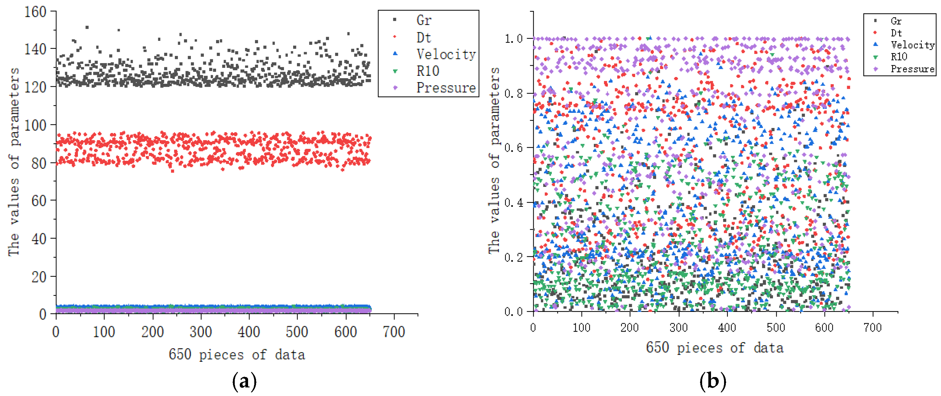
4.2. Data Standardization Processing

Since different parameters may have different units and dimensions, various data scales may lead to slow convergence speed of neural network models, and outliers significantly impact model prediction. We have normalized the data to the same range and area to eliminate these effects. Data normalization methods currently include Min-Max Normalization, Z-score Normalization, and decimal normalization. Considering that drilling is a serialization process that varies with depth, and parameters such as wave velocity, gamma, DT, and R10 do not follow a normal distribution, to reduce the impact of different orders of magnitude of each parameter on model performance, this paper adopts the Min-Max method to normalize logging and drilling data. Min-Max Normalization, or deviation normalization, is a linear transformation of raw data that results in the [0, 1] interval. The transformation function is as follows:

$$\mathrm{M}\mathrm{A}\mathrm{P}\mathrm{E}=\left({\displaystyle \frac{1}{N}}\sum _{i=1}^{\mathrm{N}} \left|{\displaystyle \frac{Y_i-{\widehat{Y}}_i}{Y_i}}\right|\right)\times 100$$

(18)

Among them, Y represents the normalized value of variable X, X_i is the value of variable X, X_min is the minimum value of variable X, and X_max is the maximum value of variable X. The normalized partial data are as follows (Figure 6):

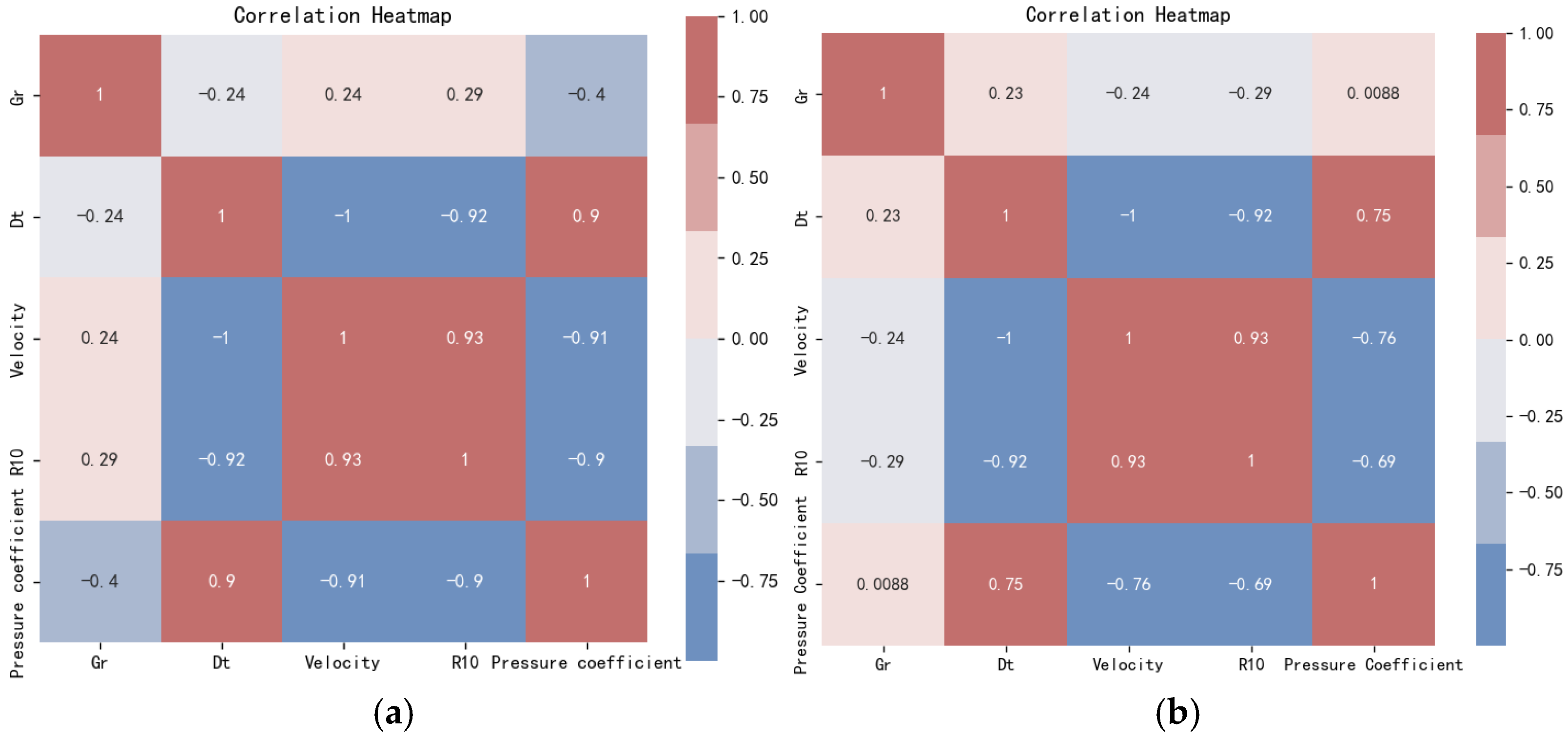
4.3. Correlation Analysis

We chose representative logging data for the construction of neural network models. Figure 7 shows the correlation matrix heatmap of various parameters and anomaly formation pressure of relief type for two sets of well-logging data. The correlation coefficients between GR, Dt, Velocity, and R10 of well A and the pore pressure coefficient are −0.4, 0.9, −0.91, and −0.9, respectively. The correlation coefficients between GR, Dt, Velocity, and R10 of well B and the pore pressure coefficient are 0.0088, 0.75, −0.76, and −0.69, respectively. The larger the absolute value of the correlation coefficient, the stronger the correlation, and the closer the correlation coefficient is to 1 or −1, the stronger the correlation. The closer the correlation coefficient is to 0, the weaker the correlation. The results indicate that the selected logging data (GR, Dt, Velocity, and R10) correlate well with the relief type’s formation pressure. Among them, the linear relationship between GR and formation pressure of relief type is weak. Due to the significant impact of shale content indicated by GR on porosity, considering the necessity of mud content and the good correlation of other logging data, the logging data of the above four parameters were selected as input variables, and corresponding measured formation pressure was designed as output variables.

4.4. Example Applications

Select 1088 core sample data from the research area to train and test the network model. The data were randomly distributed in an 8:2 ratio between the training and testing sets, with 870 datasets used for training and 218 used for testing. The output efficiency is evaluated by adjusting the number of neurons in the hidden layer and comparing the relative error between the network output and the measured formation pressure. Using the Pearson correlation coefficient method to calculate the correlation between various parameters and formation pore pressure of relief type (Figure 7), select the curve parameters with absolute correlation coefficients greater than 0.4: GR, Dt, Velocity, and R10. Construct a single-hidden-layer network structure consisting of an input layer, hidden layer, and output layer, where more minor errors indicate more stable model outputs.

We use the code to automatically adjust the number of the best hidden neurons. The network’s prediction error is minimized when the number of neurons in the hidden layer is 10. Therefore, the number of neurons in the hidden layer is determined to be 10. The learning rate, that is, the learning goal, is set at 0.001. Because the output range of the sigmoid function is between 0 and 1, it is very suitable for use as the output function of the model. It is used to output a probability value in the range of 0 to 1, for example, it is used to represent the category of two classifications or to represent the confidence. It is easy to derive; the gradient is smooth and easy to derive to prevent abrupt gradients in the process of model training. Therefore, we choose the sigmoid function as the activation function.

Once the network structure is determined, the model can be trained. By continuously adjusting, repeatedly training, and testing, a final formation pressure of relief type prediction model is established when the prediction accuracy meets the requirements. Figure 8 shows the training, validation, and testing performance of the BPNN model. Select the optimal parameter optimization model. Test data are used to validate the applicability of the model. The correlation coefficient between the measured formation pressure and the model output pressure values for 870 training sets is 0.93382218. The correlation coefficient between the measured formation pressure and the model output pressure values for 1088 datasets using this model is 0.92448. The correlation coefficient between the measured formation pressure and the model output pressure values for 1088 datasets using this model is 0.92432. The results indicate that the model has good application value in predicting the formation of pore pressure of relief type in the study area.

Use the trained BP neural network model to predict the formation pressure in the depressurization section of the well. The model’s applicability was evaluated by comparing the model’s output results with the measured formation pressure. Two wells in the study area were selected as application examples for formation pressure of relief type prediction and adaptability discussion. Figure 9 shows the predictions of the model applied to two wells. The results indicate that the average relative error of the model output from well A in the study area is within 6% (Figure 10). The average relative error of well B model output in the research area is within 6%, and there is a good correlation between the model output and the measured formation pressure, indicating high accuracy of the model output.

The BP neural network model trained using the provided downhole pressure reduction data accurately predicted the anomaly pore pressure of relief type, with an AAPE of 4.22% and an R of 0.875. When applying the equations extracted by the model to well B in the same area, further testing was conducted on the data obtained from the same training well, resulting in a predicted pore pressure of 5.44% AAPE and 0.864 R.

After analyzing the error in the formation pressure of relief type in two wells, it was concluded that the BPNN model performed well. At the same time, comparing the prediction error of the BPNN model with the support vector machine (SVM) model and Bowers model, it was found that the BPNN model had a smaller prediction error (Figure 10), and the predicted results of the BPNN model were closer to the actual pressure coefficient. This indicates that the BP neural network model can better meet the engineering requirements for predicting pressure relief type abnormal formation pressure, and has good application prospects in predicting anomaly formation pressure of relief type.

5. Discussion

In the future, more logging data should be collected, neural network parameters should be optimized, local merging should be reduced, and model prediction performance should be improved. Meanwhile, other optimization algorithms, such as genetic algorithms (GAs) (Figure 11) and particle swarm optimization algorithms, should be considered to optimize and compare with BPNN. At the same time, combine edge computing models and digital twin technology to improve the confidence of high-risk drilling environment prediction. Analyze the accuracy of predictions.

6. Summary and Conclusions

We designed and trained a neural network-based prediction model while optimizing its parameters. We adjust the model’s parameters by selecting a suitable neural network structure, including the input, hidden, and output layers, and using appropriate activation functions and optimization algorithms. By using the BP neural network to predict the anomaly formation pressure of relief type, the following conclusions were obtained:

(1)

Most stages of oil and gas exploration and development require precise prediction of formation pressure. Empirical and artificial intelligence methods have been developed to predict formation pressure. This study highlights the potential of the BP neural network (BPNN) in predicting the anomaly formation pressure of relief type and demonstrates sufficient effectiveness in prediction.

(2)

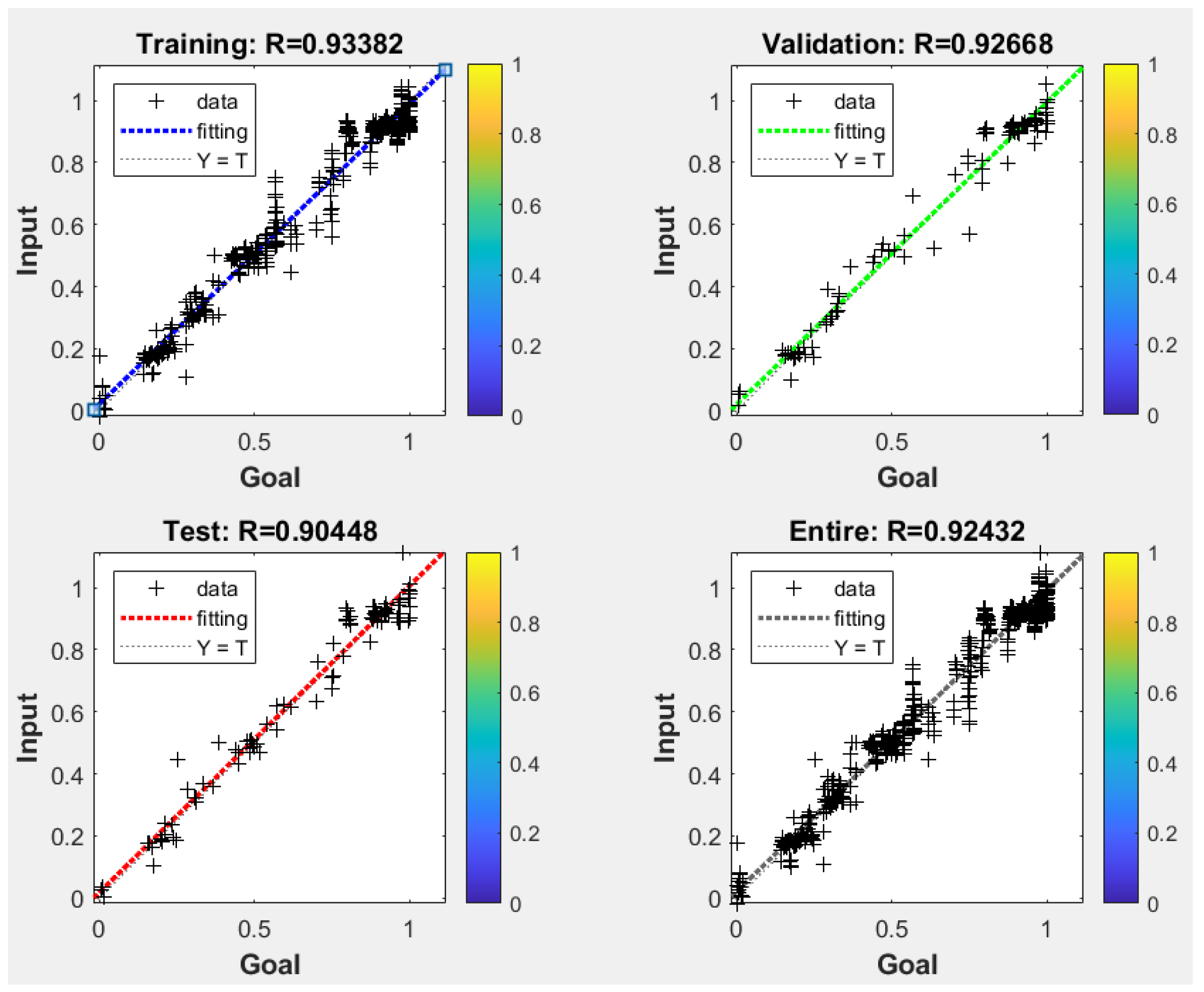
The correlation between logging parameters and the data of formation pressure of relief type indicates a good correlation between logging parameters such as GR, Dt, Velocity, and R10 and formation pressure of relief type. They are selected as input neurons. Define the number of neurons in the hidden layer as 10 through multiple optimization methods. The iteration selection is 42 to minimize the average absolute error of the validation data.

(3)

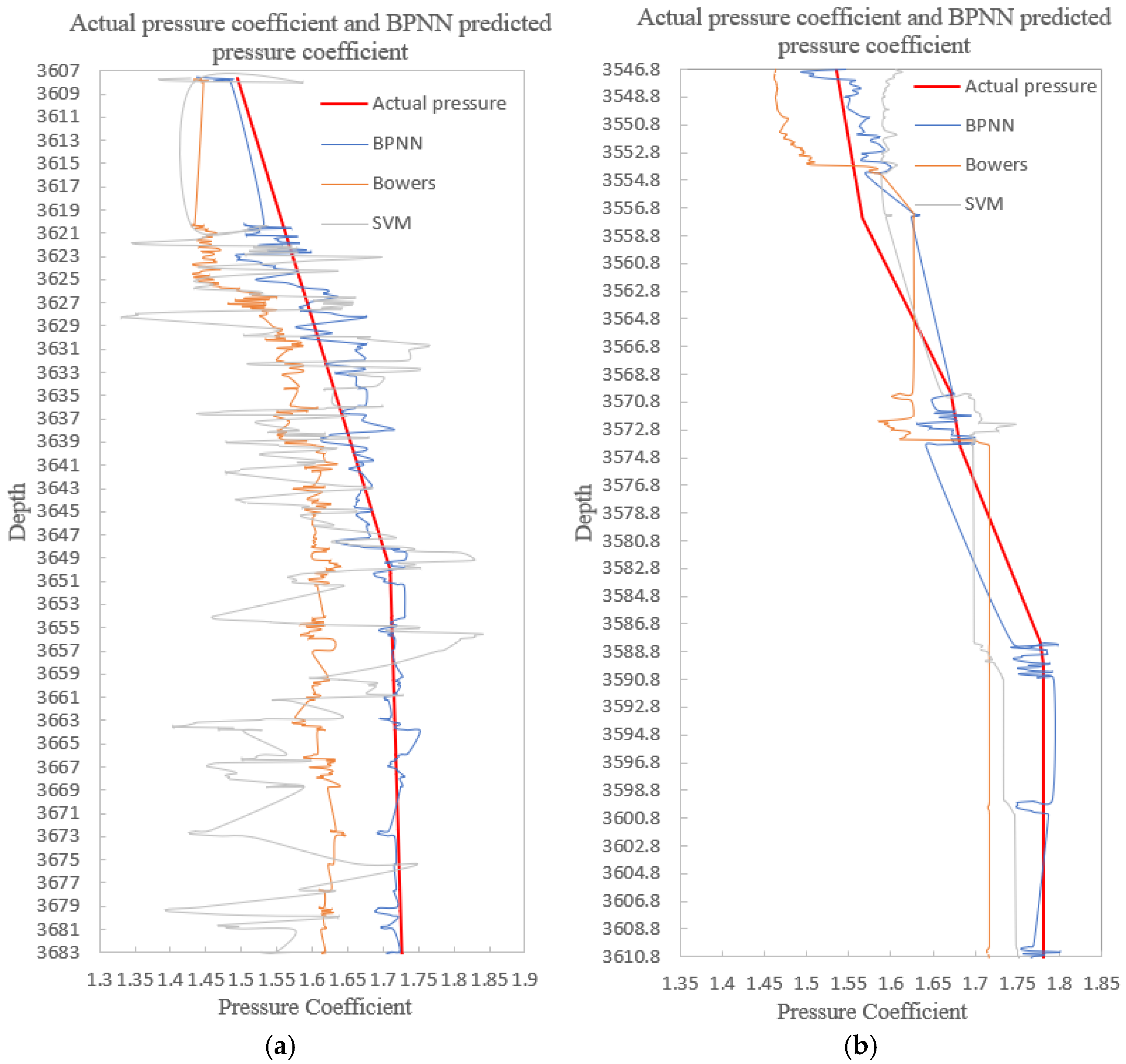
Based on the research results, a BP neural network model was trained using the provided data on the decrease in downhole pressure to accurately predict anomaly pore pressure, resulting in an AAPE of 4.22% and an R of 0.875. When applying the equations extracted by the model to well B in the same area, further testing was conducted on the data obtained from the same training well, resulting in a predicted pore pressure of AAPE of 5.44% and R of 0.864.

(4)

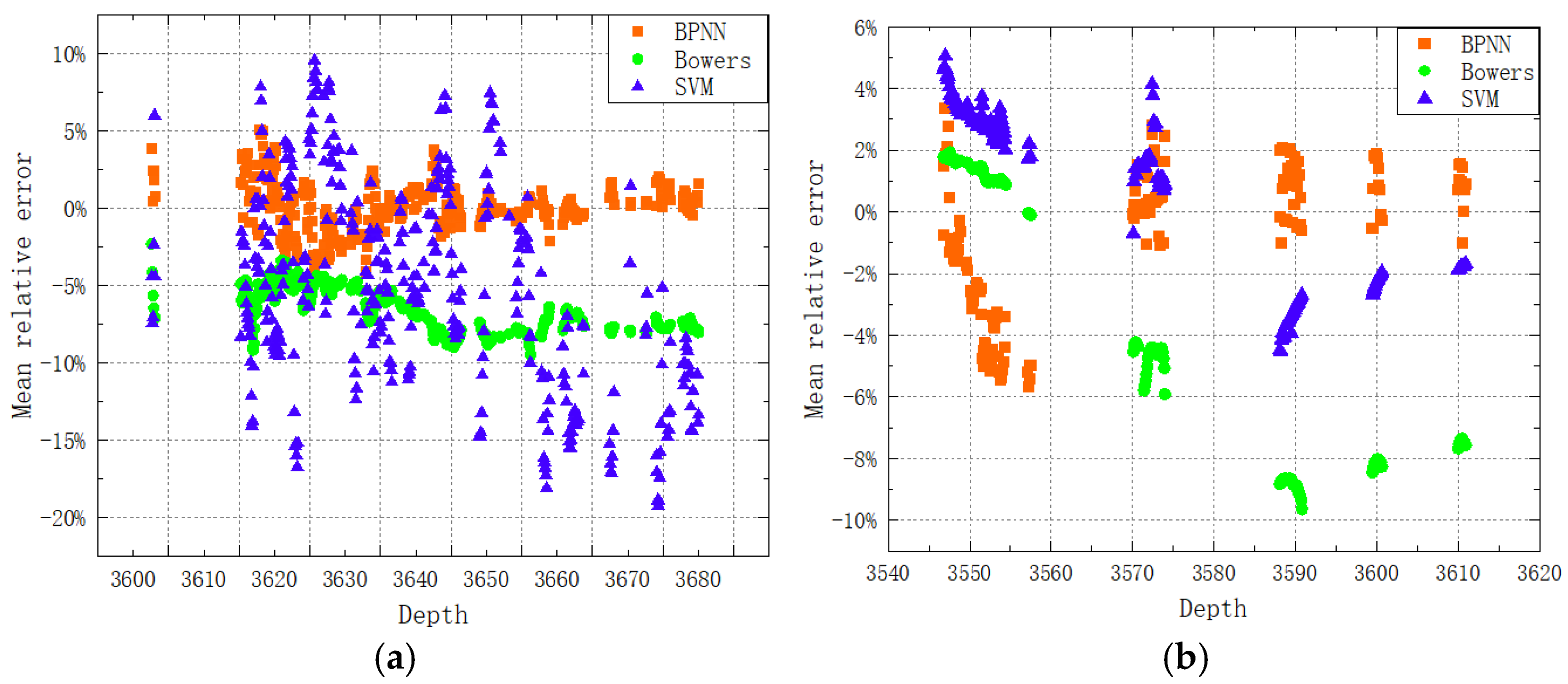
Using the BP neural network to predict pore pressure in anomaly formations with pressure relief from other sources is a relatively new method. When multiple possible factors affect the formation’s pore pressure, using BP neural network processing has significant advantages. The proposed model has several advantages in terms of accuracy and universality. Firstly, it can handle nonlinear and complex relationships between input and output variables. Secondly, it is necessary to accurately predict the formation pore pressure values of relief type through this model, as it can optimize drilling parameters such as mud weight, significantly reducing drilling costs. At the same time, comparing and observing the graph, it is found that the BPNN model has substantially better prediction performance than the traditional towers model and can better meet engineering needs.

References

1. Law, B.E.; Ulmishek, G.F.; Slavin, V.I. Abnormal Pressures in Hydrocarbon Environments. In AAPG Memoir 70; AAPG: Tulsa, OK, USA, 1998. [Google Scholar]
2. Ernanda; Primasty, A.Q.T.; Akbar, K.A. Detecting Overpressure Using the Eaton and Equivalent Depth Methods in Offshore Nova Scotia, Canada. IOP Conf. Ser. Earth Environ. Sci. 2018, 132, 012016. [Google Scholar] [CrossRef]
3. Gao, G.; Huang, Z.; Wang, Z. Study on the mechanisms of the formation of formation abnormal high-pressure. J. Xi’an Shiyou Univ. (Nat. Sci. Ed.) 2001, 20, 17. [Google Scholar]
4. Fan, H. Research and Application of a New Method for Predicting and Detecting Formation Pore Pressure. Ph.D. Thesis, China University of Petroleum, Beijing, China, 2001. [Google Scholar]
5. Law, B.E.; Spenser, C.W. Abnormal Pressures in Hydrocarbon Environments; AAPG: New York, NY, USA, 1998; pp. 1–11. [Google Scholar]
6. Neuzil, C.E. Abnormal pressures as hydrodynamic phenomena. Am. J. Sci. 1995, 295, 742–786. [Google Scholar] [CrossRef]
7. Li, W.; Chen, Z.; Huang, P.; Yu, Z.; Min, L.; Lu, X. Formation of overpressure system and its relationship with the distribution of large gas fields in typical foreland basins in central and western China. Pet. Explor. Dev. 2021, 48, 536–548. [Google Scholar] [CrossRef]
8. GB/T 26979—2011; China National Standardization Administration Committee. The Classification of Natural Gas Pool. Standards Press of China: Beijing, China, 2011.
9. Li, M. Oil and Gas Migration; Petroleum Industry Press: Beijing, China, 2006; pp. 4–11. [Google Scholar]
10. Adams, N.; Charrier, T. Drilling Engineering: A Complete Well Planning Approach; PennWell Publishing Company: Tulsa, OK, USA, 1985. [Google Scholar]
11. Rabia, H. Well Engineering & Construction; Entrac Consulting: Houston, TX, USA, 2001; ISBN 9780954108700. [Google Scholar]
12. Legkokonets, V.A.; Islamov, S.R.; Mardashov, D.V. Multifactor Analysis of Well Killing Operations on Oil and Gas Condensate Field with a Fractured Reservoir. In Proceedings of the International Forum-Contest of Young Researchers: Topical Issues of Rational Use of Mineral Resources; Taylor & Francis: London, UK, 2019; pp. 111–118. [Google Scholar]
13. Islamov, S.; Bondarenko, A.; Korobov, G.; Podoprigora, D. Complex Algorithm for Developing Effective Kill Fluids for Oil and Gas Condensate Reservoirs. Int. J. Civ. Eng. Technol. 2019, 10, 2697–2713. [Google Scholar]
14. Ganguli, S.S.; Sen, S. Investigation of Present-Day in-Situ Stresses and Pore Pressure in the South Cambay Basin, Western India: Implications for Drilling, Reservoir Development and Fault Reactivation. Mar. Pet. Geol. 2020, 118, 104422. [Google Scholar] [CrossRef]
15. Radwan, A.E.; Abudeif, A.M.; Attia, M.M.; Mohammed, M.A. Pore and Fracture Pressure Modeline Using Direct and Indirect Methods in Badri Field, Gulf of Suez, Egypt. J. Afr. Earth Sci. 2019, 156, 133–143. [Google Scholar] [CrossRef]
16. Singha, D.K.; Chatterjee, R.; Sen, M.K.; Sain, K. Pore Pressure Prediction in Gas-Hydrate Bearing Sediments of Krishna-Godavari Basin, India. Mar. Geol. 2014, 357, 1–11. [Google Scholar] [CrossRef]
17. Zhang, J. Pore Pressure Prediction from Well Logs: Methods, Modifications, and New Approaches. Earth-Sci. Rev. 2011, 108, 50–63. [Google Scholar] [CrossRef]
18. Xu, B.; Xu, H.; Yu, B.; Jing, H.; Guo, J. Application of Abnormal Formation Pressure Prediction Technologies in Junggar Basin. Xinjiang Pet. Geol. 2015, 36, 597–601. [Google Scholar]
19. Kiss, A.; Fruhwirth, R.K.; Pongratz, R.; Maier, R.; Hofstätter, H. Formation breakdown pressure prediction with artificial neural networks. In Proceedings of the SPE International Hydraulic Fracturing Technology Conference and Exhibition, Muscat, Oman, 16–18 October 2018. [Google Scholar]
20. Qian, L.; Wang, X.; Li, F.; Li, J.; Wang, J.; Qu, Y. Fillippone formula combined with equivalent medium theory to predict formation pressure. Oil Geophys. Prospect. 2018, 53, 224–229. [Google Scholar]
21. Kun, W.; Jia, L.; Lin, Y.; Wei, Y.; Wu, K.; Li, J.; Chen, Z. Artificial neural network accelerated flash calculation for compositional simulations. In Proceedings of the SPE Reservoir Simulation Conference, Galveston, TX, USA, 10–11 April 2019. [Google Scholar]
22. Li, Y.; Sun, W.; He, W.; Yang, Y.; Zhang, X.; Yan, Y. Prediction method of shale formation pressure based on pre-stack inversion. Lithol. Reserv. 2019, 31, 113–121. [Google Scholar]
23. Clifford, A.; Aminzadeh, F. Gas detection from absorption attributes and amplitude versus offset with artificial neural networks in grand bay field. In SEG Technical Program Expanded Abstracts 2011; Society of Exploration Geophysicists: Houston, TX, USA, 2011; pp. 375–380. [Google Scholar]
24. Ogiesoba, O.; Ambrose, W. Ambrosew Seismic attributes investigation of depositional environments and hydrocarbon sweet-spot distribution in Serbin Field, TaylorGroup, Central Texas. In SEG Technical Program Expanded Abstracts 2017; Society of Exploration Geophysicists: Houston, TX, USA, 2011; pp. 2274–2278. [Google Scholar]
25. Fogg, A.N. Petro-seismic classification using neural networks: UK onshore. In SEG Technical Program Expanded Abstracts 2017; Society of Exploration Geophysicists: Houston, TX, USA, 2011; pp. 1426–1429. [Google Scholar]
26. Zhang, T.F.; Tilke, P.; Dupont, E.; Zhu, L.C.; Liang, L.; Bailey, W. Generating geologically realistic 3D reservoir facies models using deep learning of sedimentary architecture with generative adversarial networks. Pet. Sci. 2019, 16, 541–549. [Google Scholar] [CrossRef]
27. Noshi, C.I.; Eissa, R.M.; Abdallar, M. An intelligent data driven approach for production prediction. In Proceedings of the Offshore Technology Conference, Houston, TX, USA, 6–9 May 2019; p. OTC-29243-MS. [Google Scholar]
28. Rui, Z.; Hu, J. Production performance forecasting method based on multivariate time series and vector autoregressive machine learning model for waterflooding reservoirs. Pet. Explor. Dev. 2021, 48, 175–184. [Google Scholar]
29. Jia, D.L.; Guo, T.; Pei, X.H.; Zhang, J.; Ye, Q.; Jin, X.G.; Tang, X. Intelligent waterflooding development of high-permeability reservoirs at the late development stage. In Proceedings of the SPE Asia Pacific Oil and Gas Conference and Exhibition, Brisbane, Australia, 29–31 October 2018; p. SPE-192067MS. [Google Scholar]
30. Zang, K.; Zhao, X.; Zhang, L.; Zhang, H.; Wang, H.; Chen, G.; Zhao, M.; Jiang, Y.; Yao, J. Current status and prospect for the research and application of big data and intelligent optimization methods in oilfield development. J. China Univ. Pet. (Ed. Nat. Sci.) 2020, 44, 28–38. [Google Scholar]
31. Liao, G.; Guo, S.; Wang, C.; Shen, Y.; Gao, Y. Pressure Relief-Type Overpressure Distribution Prediction Model Based on Seepage and Stress Coupling. Processes 2023, 11, 480. [Google Scholar] [CrossRef]
32. Adiche, S.; Larbi, M.; Toumi, D.; Bouddou, R.; Bajaj, M.; Bouchikhi, N.; Zaitsev, I. Advanced control strategy for AC microgrids: A hybrid ANN-based adaptive PI controller with droop control and virtual impedance technique. Sci. Rep. 2024, 14, 31057. [Google Scholar] [CrossRef]
33. Liu, T.; Ye, X.; Cheng, L.; Hu, Y.; Guo, D.; Huang, B.; Li, Y.; Su, J. Intelligent Pressure Monitoring Method of BP Neural Network Optimized by Genetic Algorithm: A Case Study of X Well Area in Yinggehai Basin. Processes 2024, 12, 2439. [Google Scholar] [CrossRef]
34. Sarra, Z.; Bouziane, M.; Bouddou, R.; Benbouhenni, H.; Mekhilef, S.; Elbarbary, Z.M.S. Intelligent control of hybrid energy storage system using NARX-RBF neural network techniques for microgrid energy management. Energy Rep. 2024, 12, 5445–5461. [Google Scholar] [CrossRef]
35. Zaidi, S.; Meliani, B.; Bouddou, R.; Belhadj, S.M.; Bouchikhi, N. Comparative study of different types of DC/DC converters for PV systems using RBF neural network-based MPPT algorithm. J. Renew. Energ. 2024, 1, 13. [Google Scholar] [CrossRef]
36. Berrouk, A.S.; Nandakumar, K. Special issue section on process system safety and risk engineering. Can. J. Chem. Eng. 2024, 103, 4–7. [Google Scholar] [CrossRef]
37. Abdulmalek, A.S.; Elkatatny, S.; Abdulraheem, A.; Mahmoud, M.; Abdulwahab, Z.A.; Mohamed, I.M. Pore pressure prediction while drilling using fuzzy logic. In Proceedings of the SPE kingdom of Saudi Arabia Annual Technical Symposium and Exhibition, Dammam, Saudi Arabia, 23–26 April 2018; p. SPE-192318-MS. [Google Scholar]
38. Hadi, F.; Eckert, A.; Almahdawi, F. Real-time pore pressure prediction in depleted reservoirs using regression analysis and artificial neural networks. In Proceedings of the SPE Middle East Oil and Gas Show and Conference, Manama, Bahrain, 18–21 March 2019; p. SPE-194851-MS. [Google Scholar]
39. Rashidi, M.; Hajipour, M.; Asadi, A. Correlation between static and dynamic elastic modulus of limestone formations using artificial neural networks. In Proceedings of the 52nd U.S. Rock Mechanics/Geomechanics Symposium, Seattle, WA, USA, 17–20 June 2018. [Google Scholar]
40. Rashidi, M.; Asadi, A. An artificial intelligence approach in estimation of formation pore pressure by critical drilling data. In Proceedings of the 52nd U.S. Rock Mechanics/Geomechanics Symposium, Seattle, WA, USA, 17–20 June 2018. [Google Scholar]
41. Fan, H. Analysis Methods and Applications of Abnormal Formation Pressures; Science Press: Beijing, China, 2016. [Google Scholar]
42. Bowers, G.L. Pore pressure estimation from velocity data: Accounting for overpressure mechanisms besides undercompaction. SPE Drill. Competion 1995, 10, 89–95. [Google Scholar] [CrossRef]
43. Eaton, B.A. The equation for geopressure prediction from well logs. In Proceedings of the Fall Meeting of the Society of Petroleum Engineers of AIME, Dallas, TX, USA, 28 September–1 October 1975; p. SPE-5544-MS. [Google Scholar]
44. Gamal, H.; Abdelaal, A.; Elkatatny, S. Machine learning models for equivalent circulating density prediction from drilling data. ACS Omega 2021, 8, 4363. [Google Scholar] [CrossRef] [PubMed]
45. Asadisaghandi, J.; Pejman, T. Comparative evaluation of back-propagation neural network learning algorithms and empirical correlations for prediction of oil PVT properties in Iran oilfields. J. Pet. Sci. Eng. 2011, 78, 464–475. [Google Scholar] [CrossRef]
Figure 1. Logging diagram pressure relief of sand body. The Hainan Branch of CNOOC (Hainan, China) Ltd. provided the data.
Processes 13 00616 g001
Figure 2. A well pressure relief of sand body. The Hainan Branch of CNOOC (Hainan, China) Ltd. provided the data.
Processes 13 00616 g002
Figure 3. The core steps of the BP neural network.
Processes 13 00616 g003
Figure 4. The structure of the BPNN model.
Processes 13 00616 g004
Figure 5. Prediction of formation pressure relief workflow.
Processes 13 00616 g005
Figure 6. (a) The drilling data before normalization; (b) the drilling data after normalization.
Processes 13 00616 g006
Figure 7. (a) The correlation heatmaps in well A drilling data; (b) the correlation heatmaps in well B drilling data.
Processes 13 00616 g007
Figure 8. Goodness-of-fit plot for model regression.
Processes 13 00616 g008
Figure 9. (a) Well A comparison of predicted results from different models with actual measured values; (b) well B comparison of predicted results from different models with actual measured values.
Processes 13 00616 g009
Figure 10. (a) Well A relative error between BPNN model, Bowers model, SVM model, and the actual value; (b) well B relative error between BPNN model, Bowers model, SVM model, and the actual value.
Processes 13 00616 g010
Figure 11. Genetic algorithm (GA) optimization BPNN roadmap.
Processes 13 00616 g011